| Issue |
A&A
Volume 683, March 2024
|
|
|---|---|---|
| Article Number | A171 | |
| Number of page(s) | 10 | |
| Section | The Sun and the Heliosphere | |
| DOI | https://doi.org/10.1051/0004-6361/202348657 | |
| Published online | 15 March 2024 | |
Validity of using Elsässer variables to study the interaction of compressible solar wind fluctuations with a coronal mass ejection
1
Department of Physics, University of Helsinki, PO Box 64 00014 Helsinki, Finland
e-mail: This email address is being protected from spambots. You need JavaScript enabled to view it.
2
Centre for mathematical Plasma Astrophysics, Mathematics Department, KU Leuven, Celestijnenlaan 200B Bus 2400, 3001 Leuven, Belgium
Received:
17
November
2023
Accepted:
20
January
2024
Abstract
Context. Alfvénic fluctuations, as modelled by the non-linear interactions of Alfvén waves of various scales, are seen to dominate solar wind turbulence. However, there is also a non-negligible component of non-Alfvénic fluctuations. The Elsässer formalism, which is central to the study of Alfvénic turbulence due to its ability to differentiate between parallel and anti-parallel Alfvén waves, cannot strictly separate wavemodes in the presence of compressive magnetoacoustic waves. In this study, we analyse the deviations generated in the Elsässer formalism as density fluctuations are naturally generated through the propagation of a linearly polarised Alfvén wave. The study was performed in the context of a coronal mass ejection (CME) propagating through the solar wind, which enables the creation of two solar wind regimes, pristine wind and a shocked CME sheath, where the Elsässer formalism can be evaluated.
Aims. We studied the deviations of the Elsässer formalism in separating parallel and anti-parallel components of Alfvénic solar wind perturbations generated by small-amplitude density fluctuations. Subsequently, we evaluated how the deviations cause a misinterpretation of the composition of waves through the parameters of cross helicity and reflection coefficient.
Methods. We used an ideal 2.5D magnetohydrodynamic model with an adiabatic equation of state. An Alfvén pump wave was injected into the quiet solar wind by perturbing the transverse magnetic field and velocity components. This wave subsequently generates density fluctuations through the ponderomotive force. A CME was injected by inserting a flux-rope modelled as a magnetic island into the quasi-steady solar wind.
Results. The presence of density perturbations creates a ≈10% deviation in the Elsässer variables and reflection coefficient for the Alfvén waves as well as a deviation of ≈0.1 in the cross helicity in regions containing both parallel and anti-parallel fluctuations.
Key words: magnetohydrodynamics (MHD) / turbulence / waves / Sun: corona / Sun: coronal mass ejections (CMEs) / solar wind
© The Authors 2024
 Open Access article, published by EDP Sciences, under the terms of the Creative Commons Attribution License (https://creativecommons.org/licenses/by/4.0), which permits unrestricted use, distribution, and reproduction in any medium, provided the original work is properly cited.
This article is published in open access under the Subscribe to Open model. This email address is being protected from spambots. You need JavaScript enabled to view it. to support open access publication.
1. Introduction
The origin and acceleration of the solar wind can be explained through the turbulent cascade of large-wavelength Alfvénic perturbations to kinetic scales that heat the plasma (Coleman 1968; Belcher & Davis 1971; Goldreich & Sridhar 1995; Alazraki & Couturier 1971). These Alfvén waves are generated through photospheric convective motions where the solar magnetic field footpoints are anchored (Cranmer & Van Ballegooijen 2005). The presence of Alfvénic fluctuations has been observed both in situ (Belcher & Davis 1971; D’Amicis & Bruno 2015) and remotely (Tomczyk et al. 2007), and their amplitudes have been estimated to be between 20 km s−1 and 55 km s−1 based on observations of non-thermal velocity amplitudes in the upper transition region of the Sun (Chae et al. 1998; Doyle et al. 1998). Here, “Alfvénic fluctuations” refers to perturbations polarised perpendicular to the mean magnetic field B0 that exhibit correlations between the velocity and magnetic field components. However, solar wind fluctuations also have a measurable fraction of non-Alfvénic (compressible) modes (Higdon 1984). These fluctuations can arise through non-linear wave-wave interactions of the fast, slow, and Alfvén modes (Nakariakov et al. 1997; Chandran 2005; Fu et al. 2022), from instabilities (Goldstein 1978; Derby 1978), and from turbulence driving processes. Subsequently, in situ solar wind measurements beyond the Alfvén critical point have indicated that most fluctuation power is contained in the Alfvénic modes as opposed to the compressive fluctuations (Bruno & Carbone 2013; Chen 2016). Under the assumptions that the turbulent fluctuations are small compared to the mean field, are spatially anisotropic with respect to it, and have a frequency that is low compared to the ion cyclotron frequency, Schekochihin et al. (2009) showed that the “inertial range” cascade separates into two parts: a cascade of Alfvénic fluctuations and a passive cascade of density fluctuations. This allowed us to study the cascade of Alfvénic fluctuations in the incompressible limit with Alfvénic turbulence passively interacting with the compressive fluctuations. Thus, coronal heating via Alfvénic turbulence in global simulations (Mikić et al. 1999, 2018) has been modelled in the incompressible regime through the reflection-driven turbulence model (Chandran & Perez 2019). This model is supported by numerous studies covering various aspects of the reflection-driven turbulence: the linear Alfvén wave problem (Ferraro & Plumpton 1958; Goldreich & Sridhar 1995; Velli 1993; Suzuki 2004; Sishtla et al. 2022); radial evolution of turbulence (Verdini & Velli 2007; Tenerani & Velli 2017; Zank et al. 2018); and incorporation of the turbulence model into simulations (Cranmer et al. 2007; Chandran et al. 2011; van der Holst et al. 2014). Such turbulence models approach the heating problem by considering counter-propagating Alfvén waves generated through reflections from large-scale gradients in the solar wind (Velli et al. 1989; Zhou & Matthaeus 1989), and they model the turbulent heating due to incompressible fluctuations that have been found to dominate the solar wind in the heliosphere (Tu & Marsch 1995).
An essential tool to analyse incompressible magnetohydrodynamic (MHD) turbulence is Elsässer (Elsässer 1950) formalism, which in the solar wind enables the separation of sunward and anti-sunward directed Alfvénic fluctuations based on the correlation and anti-correlation of the velocity and magnetic field. The separation of sunward and anti-sunward directed Alfvénic fluctuations enables the modelling of coronal heating via Alfvénic turbulence through the interaction of counter-propagating Alfvén waves. The significance of the Elsässer variables becomes less precise in the presence of density perturbations caused by magnetoacoustic waves. This is particularly evident when distinguishing between sunward and anti-sunward directed fluctuations (Magyar et al. 2019). Previously, Marsch & Mangeney (1987) has shown that the compressible MHD equations can be expressed through Elsässer variables with a variable density, with small-amplitude density perturbations allowing for decomposition of the variables into a purely Alfvénic and a compressive component. Therefore, Elsässer variables need not preserve their decomposition of the waves propagating in opposite directions in the compressive MHD regime. However, the usage of these variables based on their ability to separate the directionality of waves is central in the reflection-driven turbulence model and widely used in the in situ analysis of the solar wind, particularly when it can be assumed that most of the wave power lies within the Alfvénic modes (Tu et al. 1989; Grappin et al. 1990; Good et al. 2022). However, the effect of small-amplitude density fluctuations on Alfvén wave dynamics is essential to enable wave reflections sufficient to accelerate the solar wind via turbulent heating (Van Ballegooijen & Asgari-Targhi 2016). Thus, it is imperative to consider Alfvén waves mixed with density fluctuations when analysing the plasma in simulations and observational data, especially as it is not possible to exactly decompose the waves into Alfvén and non-Alfvén waves due to their non-linear mixing (Gan et al. 2022; Fu et al. 2022). Therefore, estimating the deviations in the Elsässer formalism that are introduced by the density fluctuations is important due to the non-negligible component of compressible turbulence throughout the heliosphere (Marsch & Tu 1990) and their importance in heating and accelerating the wind.
In this study, we investigate the impact of compressive density fluctuations on the Elsässer-based interpretation of the waves in the solar corona in the context of a coronal mass ejection (CME) interacting with solar wind fluctuations using MHD simulations. CMEs are transient eruptions of plasma and the magnetic field from the solar corona, and they often exhibit a three-part structure in coronagraph images consisting of a bright front of compressed coronal plasma enclosing a dark, low-density cavity (assumed to correspond to a magnetic flux rope, or FR) that contains a high-density core (Gibson & Low 2000; Kilpua et al. 2017). In this study, we employed a simulation methodology similar to the simulation described in Sishtla et al. (2023, hereafter referred to as S23), which studies the interaction of a CME with (shear) Alfvén waves in the low corona. We also self-consistently generated compressive fluctuations due to the evolution of a shear Alfvén wave continually injected at the low coronal boundary. This contrasts with the simulation reported in S23, which contains only incompressible fluctuations. In S23, a lower simulation grid resolution causes the Alfvén waves to be damped due to numerical diffusion before the density fluctuations can be generated. The density fluctuations in the simulation of this work were generated through a ponderomotive force created by the propagating Alfvén wave (Sect. 2.1). The presence of the CME is important to separating the solar wind plasma into two regimes: pristine wind upstream of the CME and a shocked CME sheath. This separation allows for an analysis of the fluctuations in the two regimes that exhibit different dynamics of the propagating wave due to the differing Alfvén and sound speeds. Upon restricting our analysis to frequencies close to the Alfvén wave frequency in the quiet wind, we found the shocked CME sheath structure in the simulation to exhibit minimal density fluctuations. This occurs as the shock compresses the upstream plasma, causing the CME sheath waves to propagate outside the frequency range we investigate. Thus, the shock appears to reset the solar wind fluctuations for the range of frequencies we study. The separation of the pristine wind from the CME sheath allowed us to study the Elsässer formalism in two regimes defined by density fluctuations through the same simulation.
The study finds the large-scale structures of the CME to be similar to those found in S23 but with the addition of density fluctuations in the simulation domain. However, we find that the small-amplitude compressive waves contribute to significant misinterpretations when analysing the Alfvénic waves using Elsässer variables. We find that Elsässer variables do not strictly allow for the separation between sunward and anti-sunward Alfvén waves in the presence of density fluctuations. The density fluctuations create a deviation of ≈10% in the Elsässer variables and the calculated reflection coefficient for the Alfvén waves and a deviation of ≈0.1 in the cross helicity in regions containing balanced fluctuations. In Sect. 2, we introduce the MHD equations and associated boundary conditions, the mechanism for Alfvén wave injection, and the CME model used in the simulations. A discussion of the density fluctuations affecting the reflection of Alfvén waves due to Alfvén velocity gradients is presented in Sect. 2.1. The validity of the Elsässer variable formulation is discussed in Sect. 3, and the deviations introduced in the cross helicity and reflection coefficient through the use of the formalism are discussed in Sect. 4. Finally, the conclusions are summarised in Sect. 5.
2. Methodology
We performed a 2.5D MHD numerical simulation assuming a radially outward magnetic field to initialise the solar wind. The MHD equations were advanced in time using the strong stability preserving (SSP) Runge-Kutta method to advance the semi-discretised equations (Pomoell & Vainio 2012). The numerical method employed the Harten–Lax–van Leer (HLL) approximate Riemann solver supplied by piece-wise, linear slope-limited interface states. The equations were solved in spherical coordinates, and the magnetic field was ensured to be divergence free to the floating point accuracy by utilising the constrained transport method (Kissmann & Pomoell 2012).
The MHD equations were integrated forward in time and in two spatial dimensions by considering a meridional plane with a radial extent of r = 1.03 R⊙ to r = 30 R⊙ and a co-latitudinal extent of θ = 10° to θ = 170°. The simulation domain, therefore, exhibits rotational invariance in the out-of-plane ϕ direction. However, the vector quantities in the MHD equations retain all three components. The magnetic field was initialised to be purely radial and directed outwards and defined by the vector potential  , where B0 = 5 G is the field strength at r = r0, and the magnetic field was then specified using B = ∇ × A. At the inner radial boundary, the density and temperature were chosen to be independent of latitude with ρ0 = 8.5 × 10⁻¹³ kg and T0 = 1.2 × 10⁶ K. We linearly extrapolated all dynamical quantities in order to enforce an outflow boundary condition at the outer radial and latitudinal boundaries. The simulation domain was defined by a non-regular grid with 1763 cells spaced logarithmically until 2.5 R⊙ and equidistantly spaced after that in the radial direction. In comparison, the simulation grid in S23 was defined by 500 cells spaced logarithmically in the radial direction. The grid contained 128 cells in the latitudinal direction both in the present simulation and in S23.
The MHD equations with the relevant physical processes of gravity and ad hoc heating that are numerically solved are given in S23. The solar wind plasma evolves by solving these MHD equations for a polytropic index of γ = 5/3. An ideal gas law specified as P = (ρ/m)kBT, where m is the mean molecular mass, kB is the Boltzmann constant, and P the pressure is used to compute the temperature T. We incorporated an additional energy source term to obtain a steady-state solar wind that approximates a Parker-like outflow (Pomoell et al. 2015; Mikić et al. 2018).
2.1. Introducing Alfvénic perturbations
Once a steady-state solar wind was achieved after advancing the MHD equations in time, we introduced linearly polarised shear Alfvén waves by perturbing the vϕ and Bϕ components at the low coronal boundary in the same manner as detailed in S23. The response of the solar wind to the introduction of the linearly polarised Alfvén wave is shown in Fig. 1. Panel a presents a simulation snapshot of the temperature (T) at ∼16.6 h after the start of the injection of the Alfvén wave. The temperature increases from 1.2 MK at the lower boundary to 1.4 MK at ≈2.5 R⊙ before decreasing. We observed compressive waves throughout the simulation, as represented by the wave-like features in panel a. To further illustrate the Alfvén and compressive waves, we included a plot of the vϕ, Bϕ, and the density fluctuation level in panels b–d, respectively, along a radial ray at a viewing angle of 125°, as annotated in panel a. To describe the propagation of density fluctuations, we defined the fluctuation in density δρ as ρ = ρ0 + δρ, where ρ0(τ) is the 10-min time-averaged density. This time averaging of the density allowed us to capture fluctuations in δρ up to ≈1.6 mHz. Panels b and c illustrate the presence of Alfvén wave modes in the simulation with the ϕ components of the magnetic field and velocity fluctuating in correlation. The initially injected Alfvén wave appears to steepen between 5 − 15 R⊙ before dissipating (panel b), with the fluctuations positively or negatively correlated with the fluctuations in Bϕ (panel c). Finally, in panel d, we observed density fluctuations throughout the simulation domain, albeit at varying levels.
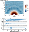 |
Fig. 1. Coronal quasi-steady state. Panel a: simulation snapshot of the plasma temperature upon the injection of a 1 mHz linearly polarised Alfvén wave, with an annotation describing the viewing angle along 125° at τ = 1000 min after the injection of the Alfvén wave. Panels b and c: out-of-plane vϕ velocity and the Bϕ magnetic field components, respectively. The fluctuations induced in the density ρ from the quasi-steady values prior to the injection of the Alfvén wave are presented in panel d. |
The dynamics of the propagating Alfvén wave in a homogeneous medium (in the co-latitudinal direction), such as in this simulation, depends on the wave polarisation. It has been shown that circularly polarised waves of arbitrary amplitudes are exact solutions of the MHD equations and exhibit no net magnetic field pressure variations as they propagate (Ferraro & Plumpton 1958; Goldstein 1978).
In contrast, linearly polarised Alfvén waves create magnetic pressure variations as they propagate, causing them to steepen (Cohen & Kulsrud 1974). The magnetic pressure gradients are balanced by an oscillating thermal pressure. Subsequently, the oscillating thermal pressure generates a ponderomotive force, which creates density fluctuations in the compressible MHD regime (Hollweg 1971; Nakariakov et al. 1997). This process of steepening (causing a temperature increase) and generating compressive waves is described through Fig. 2. In panels a–c of the figure, we present vϕ, Bϕ, and δρ/ρ along a viewing angle of 125° from the moment of Alfvén wave injection (defined here as τ = 0) until the end of the simulation (τ = 1000 min). The injected waves only reach the end of the simulation domain (30 R⊙) at τ ≈ 850 min. However, until τ ≈ 500 min, there are minimal density fluctuations as the simulation evolves towards a quasi-steady state. Then, from τ ≈ 500 min to τ ≈ 1000 min, the injected Alfvén wave grows linearly as the wave steepens (Fig. 1a plotted at τ = 1000 min), and there is continual generation of compressive wave modes. In Fig. 2d, we present a simulation snapshot of vϕ at τ = 1000 min depicting the homogeneous evolution of the injected Alfvén wave, as the crests and troughs of the wave do not have an angular dependence.
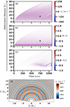 |
Fig. 2. Evolution of the solar wind as the Alfvén waves propagate through the corona. The fluctuating velocity and magnetic field components are shown in panels a and b. The density perturbations defined as δρ/ρ, where δρ = ρ − ⟨ρ⟩ and ⟨ρ⟩ is the density averaged over 10 min intervals, are shown in panel c. Panel d is a simulation snapshot of vϕ at τ = 1000 min. The dashed arrows in panels a and b highlight the apparent bifurcation of vϕ and Bϕ. |
In Fig. 2, we observed that the Alfvén waves injected at the lower boundary experience reflections at distances of 10 − 15 R⊙. This reflection is evident in the apparent bifurcation of the vϕ component (panel a), which takes two different paths, as highlighted by the dashed arrow in panel a. These paths correspond to the waves moving at their own sunward propagating phase speed v − va, where va is the Alfvén speed, and a path corresponding to reflections from the anti-sunward wave and thus propagating with phase speed v + va (Verdini & Velli 2007). This region of 10 − 15 R⊙ corresponds to background inhomogeneities in the solar wind that are sufficient to generate Alfvén wave reflections. However, the density fluctuations generated by the ponderomotive force still propagate with the same velocity as the anti-sunward Alfvén wave that generates them. Subsequently, the density fluctuations lead to the formation of gradients in the Alfvén speed that are on a spatial scale comparable to the wavelength of the Alfvén wave. In summary, the excited anti-sunward wave generates density fluctuations via the ponderomotive force, and the anti-sunward wave is then reflected by the large-scale density gradients present in the solar wind. This reflected wave interacts with not only the anti-sunward wave but also with the density fluctuations that cause further scattering.
Therefore, in this simulation, the Alfvén waves experience reflections from both large-scale background gradients as well as from small-scale variations in Alfvén velocity formed by the ponderomotive density fluctuations. In the absence of density fluctuations (as in S23), the Alfvén waves would only be reflected by background inhomogeneities.
2.2. Injecting coronal mass ejections
We chose the solar wind at t = 1000 min (Fig. 2) to represent the quasi-steady state in which we introduce the CME. We modelled the CME as a magnetic island with an FR magnetic field and a non-uniform density profile to populate the ejecta. The FR was modelled using the Soloviev solution to the Grad-Shafranov (GS) equation, which represents axisymmetric MHD equilibria of magnetised plasmas without flows such that the equilibrium condition J × B = ∇P is satisfied.
A detailed explanation of the CME model and its eruption can be found in S23. We note that we do not model the CME eruption self-consistently. Rather, the specification of thermal pressure inside the CME and the superposition of the structure on the quasi-steady solar wind results in a non-equilibrium state, causing the FR to dynamically evolve by propagating and expanding.
In Fig. 3, we present the solar wind parameters as a function of time as the CME is encountered by a virtual spacecraft located at 10 R⊙ and with a viewing angle of 125°. Before encountering the CME (i.e. in the upstream), the solar wind contains fluctuations in vϕ and Bϕ (panels a and b) along with the density and temperature fluctuations (panels c and d) as the linearly polarised Alfvén wave generates compressive waves. The arrival of the CME is characterised by the CME-driven leading shock, as seen by the simultaneous jump in radial velocity, density, temperature, and magnetic field. Following the shock is the CME sheath, which is the compressed region of plasma driven by the propagating and expanding CME. We observed solar wind fluctuations, evident as variations in vϕ and Bϕ; they are present in the upstream and in the CME sheath. Also, a local enhancement in density at t ≈ 62 min corresponding to a pile-up compression region (PUC; Das et al. 2011) is noticeable in the sheath. Finally, the spacecraft encounters the FR characterised by the smooth, large-scale rotation of the magnetic field’s Bθ component. Hence, Fig. 3 demonstrates the large-scale features typically observed in association with CMEs, namely, a shock, sheath, FR, and PUC.
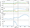 |
Fig. 3. Measurement of plasma parameters by a virtual spacecraft located at 10 R⊙ and with a viewing angle of 125°. The vertical lines delineate the upstream, sheath, and FR intervals encountered by the spacecraft. |
The modelling and analysis of a similar CME propagating in a solar wind containing only incompressible fluctuations is described in S23. In that study, the authors describe the transmission of upstream solar wind fluctuations into the CME sheath and the effect of the fluctuation frequency on the CME shock formation. The current simulation presents the evolution of the same CME in a solar wind containing compressible fluctuations. This distinction is illustrated in Fig. 4 with simulation snapshots of the density fluctuations (δρ/ρ) at t = 70 min. The snapshot in panel a shows the CME passage in a wind containing only incompressible waves. In panel b, the solar wind contains density fluctuations as well, as described in Sect. 2.1. The CME structure, on large scales, is similar in both simulation runs, and the CME deflects in the same direction. The primary and stark difference between the two simulations is the density fluctuations, which are ubiquitous in both the pristine wind and in the CME sheath and clearly visible in panel b where compressible fluctuations are present.
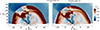 |
Fig. 4. Simulation snapshots of density fluctuations at t = 70 min as the CME propagates through the solar wind. Panel a depicts the case from S23 where no compressible fluctuations exist, and panel b depicts the solar wind from the present study containing both Alfvénic and compressible fluctuations. Panel b is annotated with the viewing angles corresponding to the CME flank (160°) and head-on (125°). |
The presence of density perturbations and their interaction with the CME is presented in Fig. 5. Panels a and b show the perturbations in density δρ/ρ for viewing angles of 160° (CME flank) and 125° (CME head-on), respectively. In the pristine solar wind, we observed the density fluctuations in a manner consistent with Fig. 2c, that is, as seen by the region of enhanced density perturbations near 10 R⊙ (annotated with (i)). When the density fluctuations encounter the CME-driven shock (annotated with (ii)), their frequency increases as the shock compresses the plasma. Thus, we observed minimal perturbations of the 10-min averaged density perturbations in the CME flanks (panel a) compared to the pristine solar wind. This indicates predominantly higher frequency density fluctuations as the upstream waves are compressed at the shock. Similarly, when viewing the CME head-on (panel b), we saw a region after the shock where the fluctuations propagate prior to encountering the FR leading edge (annotated with (iii)). This can also be observed in Fig. 4b, where one can observe density fluctuations along 125° prior to the FR leading edge. The density fluctuations start recovering after the passage of the FR, as the Alfvén waves are continually injected at the lower boundary.
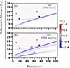 |
Fig. 5. Ten-minute averaged density perturbations δρ/ρ are presented for viewing angles of 160° (flank, panel a), and 125° (head-on, panel b). The annotations denote enhanced perturbations near 10 R⊙ in the quiet wind (i), the CME shock (ii), and the FR leading edge (iii). |
3. On the validity of the Elsässer formalism
The simulation described in Sect. 2 characterises a wind with primarily Alfvén waves and small-amplitude density fluctuations (without magnetosonic waves). As the properties of the solar wind fluctuations that have entered the CME sheath are primarily determined by their interaction with the CME shock (discussed in S23), the sheath similarly contains Alfvén waves mixed with density fluctuations. In this section, we discuss the limitations of Elsässer variables in describing such a plasma.
The Alfvénic nature (or Alfvénicity) of the waves is contained in the v − B correlation that allows us to represent the waves as the fluctuating part of  . In an incompressible medium, plasma exhibits full Alfvénic behaviour, with all wave modes as shear Alfvén waves expressed using Elsässer variables. Additionally, the z± variables define wave directionality, that is, sunward or anti-sunward. However, the density fluctuations in the upstream solar wind and downstream of the CME-driven shock first required us to verify the Alfvénicity of the waves. In Fig. 6, we show the Pearson correlation coefficient (PCC) computed for a 10-min averaging period and the corresponding p-value of the PCC along viewing angles of 160° (CME flank) and 125° (CME head-on). In the figure, the PCC is calculated between vϕ and Bϕ and can denote anti-correlation (PCC ∈ [ − 1, 0] with −1 indicating perfect anti-correlation), positive correlation (PCC ∈ [0, 1]), or no correlation (PCC = 0). The presence of correlation signifies the Alfvénic nature of the flows. The associated p-value is the probability of finding a correlation given that the parameters were uncorrelated initially (null hypothesis). Thus, in panels b and d, the locations with a p-value larger than 0.05 imply the probability of a false correlation as being greater than 5%.
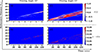 |
Fig. 6. Pearson correlation coefficients (panels a and c) and the corresponding p-values (panels b and d) along viewing angles of 160° (flank) and 125° (head-on). |
Figure 6 shows a predominance of highly anti-correlated (anti-sunward propagating) waves except near the CME shock, which coincides with locations of enhanced density (Fig. 5). The associated p-values confirm the presence of non-Alfvénic and positively correlated waves in these regions. However, the PCC values cannot be trusted around the CME shock (panels a and b) and near the FR (panels c and d), as indicated by the greater than 0.05 p-values. These regions of high p-values are locations where the plasma is quickly compressed either by the shock or the FR ejecta compressing the wind ahead of it.
If we suppose the simulation had an instability, such as the parametric decay instability (PDI; Sagdeev & Galeev 1969; Derby 1978; Goldstein 1978; Shoda et al. 2018; Chandran 2018; Sishtla et al. 2022), driving small-amplitude density fluctuations through the formation of MHD sound waves, we might still expect v − B correlations, but the presence of the magnetosonic wave would lead to the wind not being purely Alfvénic. However, specifying how density fluctuations form in the present simulation (through the ponderomotive force) without the additional magnetosonic waves ensures that the observed v − B correlation is in agreement with the presence of shear Alfvén waves, thus simplifying the definition of “Alfvénicity” in this context. Therefore, this confirmation of the Alfvénic nature of the waves supports our understanding that the solar wind fluctuations in our simulation combine shear Alfvén waves with density fluctuations. With this understanding confirmed, we could then investigate whether the directionality of the waves (sunward or anti-sunward propagating) is still captured by the definition of the Elsässer variables. Since the imposed fluctuations are confined to the ϕ direction, we analysed the  component of the Elsässer variables:
 (1)
(1)
Without density fluctuations, the  and
and  variables would denote anti-sunward and sunward fluctuations, respectively. If we assume small-amplitude density fluctuations (δρ ≪ ρ0), we can write
 (2)
(2)
using a Taylor series expansion. Here,  indicates the Elsässer variable in an incompressible medium and Δ is the leading order deviation due to the density fluctuations. Such an analysis has been performed by Magyar et al. (2019), and they showed that even in the absence of sunward fluctuations, the magnetoacoustic waves are necessarily described by both
  , as the v − B correlations are not exact for non-Alfvén waves. Without making assumptions of the small-amplitude nature of the density fluctuations, we defined ϵ to quantify the difference between the Elsässer variables with and without density fluctuations,
 (3)
(3)
where ρ = ρ0 + δρ. The ϵ parameter is calculated in Fig. 7 for both the ϕ (panels a and c) and θ (panels b and d) directions along the viewing angles of 160° (flank) and 125° (head-on). In the upstream solar wind, we saw the presence of wave-like specks of ϵϕ (panels a and c), which appear to follow the pattern of density fluctuations in Fig. 5. The region of enhanced ϵϕ near 10 R⊙ coincides with the location of enhanced density fluctuations in Figs. 2c and 5. In panels b and d, we observed no ϵθ in the upstream wind since Bθ = 0. After the CME shock transition (panels a and b), we observed negligible or zero ϵϕ, θ, as the plasma compression at the shock caused negligible δρ/ρ in the 10-min averaging interval we considered. As the solar wind recovered, we started observing some ϵϕ at lower heliocentric distances that coincide with locations in Fig. 5a where density perturbations start propagating. A similar behaviour was observed when viewing the CME head-on (panels c and d), where we observed enhanced ϵϕ, θ in locations of Alfvénic waves (Fig. 6) containing compressed plasma (Fig. 5b) before encountering the FR. In Fig. 7, the ϵ magnitude is about 5 − 10 km s−1 in the pristine solar wind at locations with density fluctuations (such as the region annotated as (i) in Fig. 5) and approximately 25 km s−1 close to the shock and CME sheath (near the region annotated as (ii) in Fig. 5). We note that the definition of the ϵ parameter in Eq. (3) depends on the averaging interval used to calculate ρ0.
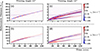 |
Fig. 7. Deviations in the Elsässer variables due to density fluctuations. The deviations (ϵ) as defined in Eq. (3) are shown for the ϕ (panels a and c) and θ (panels b and d) directions along viewing angles of 160° and 125°. |
The parameter ϵθ, ϕ indicates that even in the absence of either sunward or anti-sunward waves, we would still see a minimum value of non-zero  . To compare how the 5 − 10 km s−1 margin of deviation (ϵ) interferes with our interpretation of directionality from the Elsässer variables, we plotted the complete Elsässer variables for the ϕ and θ directions at a viewing angle of 160° in Fig. 8. Panel a depicts the transmission of the upstream anti-sunward Elsässer variable into the CME sheath, leading to the formation of CME sheath fluctuations. The fluctuations in the CME sheath exhibit a high frequency (short wavelength) due to compression by the CME shock (Vainio & Schlickeiser 1998, 1999; Sishtla et al. 2023). The accompanying sunward component (panel b) is similarly transferred downstream, with the shock compression being less prominent for such waves. We direct readers to S23 for a detailed analysis of the transmission of upstream solar wind fluctuations into the CME sheath and their subsequent influence on the CME sheath’s formation. In the upstream wind, the
  component is present in locations < 10 R⊙ as the anti-sunward wave is reflected from the large-scale density gradient. The Elsässer variables in the θ direction (panels c and d) indicate the absence of fluctuations in the pristine wind, as the injected Alfvén wave was polarised in the ϕ direction. However, in the shock neighbourhood, the plasma experiences large flows, as seen by the enhanced
  prior to the wave-like features observed after the passage of these large flows. These large flows are generated as a consequence of the non-radial shock formed by the draping of field lines around the FR. The
  component shows fluctuations downstream of the shock with a comparable amplitude and propagation velocity as
  . We note that such wave-like features in
  are absent when only incompressible shear Alfvén waves are present in the upstream wind (as in S23), indicating that they might be generated as a result of the scattering of ϕ polarised Alfvén waves by the density fluctuations.
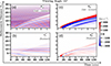 |
Fig. 8. Elsässer variables along the ϕ and θ directions shown for a viewing angle of 160° and an injected Alfvénic fluctuation frequency of 1 mHz. |
Focusing on the ϕ direction (Figs. 8a and b), we observed that the anti-sunward fluctuations have an amplitude of ≈100 − 250 km s−1, while the sunward components are ≈50 km s−1. Comparing with the regions of non-zero ϵϕ in Fig. 7a, which have a 5 − 10 km s−1 margin of ϵ, results in a ≈4% (anti-sunward) and ≈10% (sunward) deviation margin near 10 R⊙, where we observed enhanced density fluctuations. This maximum of the deviation margins is obtained through accounting for only density fluctuations with time periods of ten minutes, as dictated by the averaging interval. Therefore, shear Alfvén waves in a solar wind plasma containing density fluctuations at a level of δρ/ρ ≈ 0.1 − 0.25 cannot exactly be decomposed into sunward and anti-sunward components. The deviations become more pronounced as the density perturbations increase in amplitude (Eq. (2)). For the case of density fluctuations at smaller amplitude levels, such as in this simulation, one can still observe a non-negligible difference of ≈4%−10% in the overall amplitude of the Alfvénic waves.
4. Composition of the Alfvénic fluctuations
A significant utility of Elsässer variables in the analysis of incompressible fluctuations is revealing the composition of waves in the plasma, for example, through the cross helicity and reflection coefficient. With the assumption of an incompressible plasma, cross helicity is a rugged invariant (Matthaeus & Goldstein 1982) and can therefore track the evolution of sunward and anti-sunward Alfvén waves in the plasma. In this section, we investigate the misinterpretations caused by the cross helicity and reflection coefficient measures due to the deviations in the Elsässer formalism generated by the presence of density fluctuations.
4.1. Cross helicity
The cross helicity parameter (σc) describes the alignment between the Elsässer variables (z±) and measures the difference in power between the counter-propagating Alfvénic fluctuations. It is defined as
 (4)
(4)
For simplicity, if we restrict ourselves to the ϕ direction,
 (5)
(5)
We can simplify σc, ϕ further using Eq. (2) to obtain
 (6)
(6)
 (7)
(7)
By writing the result in the form
 (8)
(8)
a non-trivial dependence of the cross helicity on δρ becomes evident. If only sunward ( ) or anti-sunward (
 ) waves are present, then Eq. (8) still reduces to 1 or −1, respectively. Instead, if the system exhibits a balanced distribution of waves (i.e.
  ), then Eq. (8) reduces to −|Δ|/zϕ, 0. Assuming a solar wind similar to Figs. 7 and 8 with |Δ|≈ϵϕ ≈ 15 km s−1 and zϕ, 0 ≈ 100 km s−1, we can calculate −|Δ|/zϕ, 0 = −0.15, which would be a noticeable deviation from the expected zero value.
In Figs. 9a and b, we show the cross helicity with the full density ρ and the deviation in the cross helicity calculations when assuming incompressibility using ρ0, respectively. Panel a indicates that the plasma predominantly contains anti-sunward fluctuations (σc, ϕ = −1) beyond 10 R⊙ in the pristine wind. There are regions containing sunward fluctuations (σc, ϕ = 1) in the pristine wind at distances of less than 10 R⊙. The region downstream of the shock contains regions that possess all three categories: sunward, anti-sunward, and balanced fluctuations (σc, ϕ = 0). Panel b describes the cross helicity to have a deviation of ≈0.1 in the pristine wind, especially around 10 R⊙, where we have significant density fluctuations.
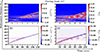 |
Fig. 9. Effect of density fluctuations on cross helicity and the reflection coefficient. The figure presents the cross helicity (a) and the reflection coefficient (c) for the full density ρ = ρ0 + δρ. We evaluated the deviations in these calculations when considering only the mean density ρ0 in panels b and d. |
4.2. Reflection coefficient
The reflection coefficient captures the fraction of z− reflected to form z+ (or vice versa). Thus, we can define the reflection coefficient to be
 (9)
(9)
Then, for a given ℛ, we can find the number of sunward waves (|z+|) generated due to the propagating anti-sunward waves (|z−|) (or vice versa). Similarly, when restricting ourselves to the ϕ direction,
 (10)
(10)
This implies that even in the absence of any sunward fluctuations ( ), we get ℛ > 0 since |Δ|≥0.
Figures 9c and d show the reflection coefficient with the full density (ρ) and the deviation assuming incompressibility (ρ0), respectively. In the pristine solar wind, we expect predominantly anti-sunward fluctuations (ℛ = 0) except in locations < 10 R⊙, where we encounter some sunward fluctuations as well (Figs. 8a and b). Figure 9c validates these conclusions with ℛ = 0 at > 10 R⊙ but ℛ ≈ 0.5 − 0.8 at < 10 R⊙ in the pristine wind. We observed specks of higher ℛ at all distances in the pristine wind corresponding to the density fluctuations observed in Fig. 5. The presence of density fluctuations generates a deviation of ≈0.1 in ℛ, as seen in Fig. 9d. The similar amplitudes of the Elsässer variables downstream of the CME shock result in higher values of ℛ along with the deviations due to the density fluctuations. If we consider the location near 10 R⊙, we observe an ℛ ≈ 0.5 − 0.7 with a deviation of ≈0.05, which corresponds to a difference of ≈7%−10% in the reflection coefficient. Therefore, this analysis reveals that if we transition to a solar wind containing small-amplitude compressive wave modes (δρ/ρ ≤ 0.25 in the pristine wind), then we overestimate the reflection coefficient by ≈7%−10%. We note that Alfvén waves are reflected by density fluctuations due to the resulting enhancements in the Alfvén velocity gradients (Van Ballegooijen & Asgari-Targhi 2016). Thus, the deviations in ℛ discussed in this section do not refer to physical reflections of the Alfvén waves that would occur in such a medium. Instead, they refer to the numerical deviations introduced by the density fluctuations in the calculations in Eq. (10).
5. Conclusion
This study has described the limitations of using Elsässer variables to analyse Alfvénic fluctuations interacting with a CME in the presence of small-amplitude density fluctuations. In particular, we have discussed the misinterpretations caused by the Elsässer formalism when separating counter-propagating Alfvén waves in the compressive plasma. In our simulation, the compressible fluctuations in the solar wind evolved naturally through the decay of a linearly polarised Alfvén wave injected at the lower coronal boundary. The CME was introduced into the simulation by modelling the FR using the Grad-Shafranov equation and populating this magnetic ejecta with a non-uniform density profile in order to ensure a smooth transition to the solar wind without abrupt changes. We found the solar wind plasma to be largely Alfvénic in nature and to exhibit strong v − B correlations. The fluctuations in the pristine solar wind are transferred downstream of the CME shock into the sheath where the ϕ polarised Alfvén waves are scattered further in the θ direction due to density fluctuations. By confining ourselves to observing frequencies around that of the injected Alfvén wave, the compression of plasma at the CME shock resulted in δρ/ρ ≈ 0 around the frequency range we investigated. This allowed us to investigate the deviations caused by the Elsässer formalism due to the density fluctuations in the pristine wind, which has a maximum of δρ/ρ ≈ 0.25 and contrasts with the CME shock where we would have a minimal δρ/ρ.
The small-amplitude nature of the density fluctuations was validated through Fig. 6, which confirms that the solar wind is dominantly Alfvénic in nature. This implies that most of the wave power lies in the Alfvénic fluctuations. Subsequently, upon defining a parameter to quantify the difference in the Elsässer variables with and without density fluctuations in Eq. (3), we found the density fluctuations generate a maximum of ≈15 km s−1 deviations in the Elsässer variables in a region of the pristine wind where δρ/ρ ≈ 0.25. This contributes to a difference of ≈4%−10% in the amplitude of anti-sunward and sunward Elsässer variables. This deviation in the Elsässer formalism further cascades into our interpretation of the composition of Alfvénic fluctuations as described in Sect. 4. We find no deviations if we only have sunward or anti-sunward fluctuations. However, in regions containing both counter-propagating Alfvénic fluctuations, the cross helicity calculations are deviated by ≈0.1. Similarly, the reflection coefficient is overestimated by a maximum of ≈10% due to the compressible wave modes. Therefore, this study attempted to quantify the misinterpretations introduced by the Elsässer formalism when analysing a highly Alfvénic solar wind where the Alfvénic components drive the compressive density fluctuations. This small-amplitude nature of the density fluctuations enables us to decompose the Elsässer variables into the compressible and incompressible components, as in Eq. (2). These features of high Alfvénicity and low δρ/ρ are similar to the properties found in the heliospheric wind (Bruno & Carbone 2013; Chen 2016), which allows for the Elsässer formalism-based in situ studies of solar wind plasma. While the inability of the Elsässer formalism to exactly separate the counter-propagating Alfvénic waves in the presence of magnetoacoustic wavemodes is known (Marsch & Mangeney 1987; Magyar et al. 2019), in this study, we attempted to quantise this interpretation in a more realistic simulation of a CME interacting with the solar wind.
In a broader scenario, apart from the ponderomotive density fluctuations, there are also magnetosonic waves present that contribute to the driving of density fluctuations. Furthermore, the correlations between velocity and magnetic field (v − B) are not exact, resulting in regions in Fig. 6 where Alfvénic behaviour is absent. Additionally, the generation of density fluctuations involves multiple sources and entails non-linear interactions. In this scenario, it becomes complex to separate the Alfvén waves from non-Alfvén waves in the spatio-temporal domain (Gan et al. 2022; Fu et al. 2022). However, if we further confine ourselves to specific regions that exhibit strong v − B correlations, the non-zero δρ/ρ still generate quantifiable deviations in the Elsässer formalism and their derived quantities, as we have shown. Thus, in the use of Elsässer variables to analyse the plasma, it is imperative to note the possible amplitudes of density fluctuations and find their significance to the calculated z± variables. Such a consideration would allow us to confidently use Elsässer variables while being aware of the uncertainty in our calculations. For instance, in our simulation, we can mathematically find the anti-sunward waves to be ≈50 km s−1 with a maximum deviation of ≈5 − 10 km s−1. Therefore, even though we have a compressible plasma, we can still comment on the presence of some sunward Alfvénic fluctuations without knowing the specific means through which this reflected wave is generated.
Acknowledgments
The work has been supported by the Finnish Centre of Excellence in Research on Sustainable Space (FORESAIL; grant no. 336807). This is a project under the Academy of Finland, and this research has been supported by the European Research Council (SolMAG; grant no. 724391) as well as Academy of Finland project SWATCH (343581).
References
- Alazraki, G., & Couturier, P. 1971, A&A, 13, 380 [NASA ADS] [Google Scholar]
- Belcher, J., & Davis, L., Jr. 1971, J. Geophys. Res., 76, 3534 [NASA ADS] [CrossRef] [Google Scholar]
- Bruno, R., & Carbone, V. 2013, Liv. Rev. Sol. Phys., 10, 1 [Google Scholar]
- Chae, J., Schühle, U., & Lemaire, P. 1998, ApJ, 505, 957 [NASA ADS] [CrossRef] [Google Scholar]
- Chandran, B. D. 2005, Phys. Rev. Lett., 95, 265004 [NASA ADS] [CrossRef] [Google Scholar]
- Chandran, B. D. 2018, J. Plasma Phys., 84, 905840615 [CrossRef] [Google Scholar]
- Chandran, B. D., & Perez, J. C. 2019, J. Plasma Phys., 85, 905850409 [NASA ADS] [CrossRef] [Google Scholar]
- Chandran, B. D., Dennis, T. J., Quataert, E., & Bale, S. D. 2011, ApJ, 743, 197 [NASA ADS] [CrossRef] [Google Scholar]
- Chen, C. 2016, J. Plasma Phys., 82, 535820602 [NASA ADS] [CrossRef] [Google Scholar]
- Cohen, R. H., & Kulsrud, R. M. 1974, Phys. Fluids, 17, 2215 [NASA ADS] [CrossRef] [Google Scholar]
- Coleman, P. J., Jr. 1968, ApJ, 153, 371 [NASA ADS] [CrossRef] [Google Scholar]
- Cranmer, S., & Van Ballegooijen, A. 2005, ApJS, 156, 265 [NASA ADS] [CrossRef] [Google Scholar]
- Cranmer, S. R., Van Ballegooijen, A. A., & Edgar, R. J. 2007, ApJS, 171, 520 [NASA ADS] [CrossRef] [Google Scholar]
- D’Amicis, R., & Bruno, R. 2015, ApJ, 805, 84 [Google Scholar]
- Das, I., Opher, M., Evans, R., Loesch, C., & Gombosi, T. I. 2011, ApJ, 729, 112 [NASA ADS] [CrossRef] [Google Scholar]
- Derby, N. F., Jr. 1978, ApJ, 224, 1013 [NASA ADS] [CrossRef] [Google Scholar]
- Doyle, J., Banerjee, D., & Perez, M. 1998, Sol. Phys., 181, 91 [NASA ADS] [CrossRef] [Google Scholar]
- Elsässer, W. M. 1950, Phys. Rev., 79, 183 [CrossRef] [Google Scholar]
- Ferraro, C. A., & Plumpton, C. 1958, ApJ, 127, 459 [Google Scholar]
- Fu, X., Li, H., Gan, Z., Du, S., & Steinberg, J. 2022, ApJ, 936, 127 [NASA ADS] [CrossRef] [Google Scholar]
- Gan, Z., Li, H., Fu, X., & Du, S. 2022, ApJ, 926, 222 [NASA ADS] [CrossRef] [Google Scholar]
- Gibson, S., & Low, B. 2000, J. Geophys. Res.: Space Phys., 105, 18187 [NASA ADS] [CrossRef] [Google Scholar]
- Goldreich, P., & Sridhar, S. 1995, ApJ, 438, 763 [Google Scholar]
- Goldstein, M. L. 1978, ApJ, 219, 700 [NASA ADS] [CrossRef] [Google Scholar]
- Good, S. W., Hatakka, L. M., Ala-Lahti, M., et al. 2022, MNRAS, 514, 2425 [NASA ADS] [CrossRef] [Google Scholar]
- Grappin, R., Mangeney, A., & Marsch, E. 1990, J. Geophys. Res.: Space Phys., 95, 8197 [NASA ADS] [CrossRef] [Google Scholar]
- Higdon, J. 1984, ApJ, 285, 109 [NASA ADS] [CrossRef] [Google Scholar]
- Hollweg, J. V. 1971, J. Geophys. Res., 76, 5155 [Google Scholar]
- Kilpua, E., Koskinen, H. E., & Pulkkinen, T. I. 2017, Liv. Rev. Sol. Phys., 14, 1 [Google Scholar]
- Kissmann, R., & Pomoell, J. 2012, SIAM J. Sci. Comput., 34, A763 [NASA ADS] [CrossRef] [Google Scholar]
- Magyar, N., Van Doorsselaere, T., & Goossens, M. 2019, ApJ, 873, 56 [NASA ADS] [CrossRef] [Google Scholar]
- Marsch, E., & Mangeney, A. 1987, J. Geophys. Res.: Space Phys., 92, 7363 [NASA ADS] [CrossRef] [Google Scholar]
- Marsch, E., & Tu, C.-Y. 1990, J. Geophys. Res.: Space Phys., 95, 11945 [NASA ADS] [CrossRef] [Google Scholar]
- Matthaeus, W. H., & Goldstein, M. L. 1982, J. Geophys. Res.: Space Phys., 87, 6011 [NASA ADS] [CrossRef] [Google Scholar]
- Mikić, Z., Linker, J. A., Schnack, D. D., Lionello, R., & Tarditi, A. 1999, Phys. Plasmas, 6, 2217 [Google Scholar]
- Mikić, Z., Downs, C., Linker, J. A., et al. 2018, Nat. Astron., 2, 913 [Google Scholar]
- Nakariakov, V., Roberts, B., & Murawski, K. 1997, Sol. Phys., 175, 93 [NASA ADS] [CrossRef] [Google Scholar]
- Pomoell, J., & Vainio, R. 2012, ApJ, 745, 151 [NASA ADS] [CrossRef] [Google Scholar]
- Pomoell, J., Aran, A., Jacobs, C., et al. 2015, J. Space Weather Space Clim., 5, A12 [NASA ADS] [CrossRef] [EDP Sciences] [Google Scholar]
- Sagdeev, R. Z., & Galeev, A. A. 1969, Nonlinear Plasma Theory (New York: Benjamin) [Google Scholar]
- Schekochihin, A., Cowley, S., Dorland, W., et al. 2009, ApJS, 182, 310 [NASA ADS] [CrossRef] [Google Scholar]
- Shoda, M., Yokoyama, T., & Suzuki, T. K. 2018, ApJ, 860, 17 [NASA ADS] [CrossRef] [Google Scholar]
- Sishtla, C. P., Pomoell, J., Kilpua, E., et al. 2022, A&A, 661, A58 [NASA ADS] [CrossRef] [EDP Sciences] [Google Scholar]
- Sishtla, C. P., Pomoell, J., Vainio, R., Kilpua, E., & Good, S. 2023, A&A, 679, A54 [NASA ADS] [CrossRef] [EDP Sciences] [Google Scholar]
- Suzuki, T. K. 2004, MNRAS, 349, 1227 [NASA ADS] [CrossRef] [Google Scholar]
- Tenerani, A., & Velli, M. 2017, ApJ, 843, 26 [Google Scholar]
- Tomczyk, S., McIntosh, S., Keil, S., et al. 2007, Science, 317, 1192 [NASA ADS] [CrossRef] [Google Scholar]
- Tu, C.-Y., & Marsch, E. 1995, Space Sci. Rev., 73, 1 [Google Scholar]
- Tu, C.-Y., Marsch, E., & Thieme, K. 1989, J. Geophys. Res.: Space Phys., 94, 11739 [NASA ADS] [CrossRef] [Google Scholar]
- Vainio, R., & Schlickeiser, R. 1998, A&A, 331, 793 [NASA ADS] [Google Scholar]
- Vainio, R., & Schlickeiser, R. 1999, A&A, 343, 303 [NASA ADS] [Google Scholar]
- Van Ballegooijen, A., & Asgari-Targhi, M. 2016, ApJ, 821, 106 [NASA ADS] [CrossRef] [Google Scholar]
- van der Holst, B., Sokolov, I. V., Meng, X., et al. 2014, ApJ, 782, 81 [Google Scholar]
- Velli, M. 1993, A&A, 270, 304 [NASA ADS] [Google Scholar]
- Velli, M., Grappin, R., & Mangeney, A. 1989, Phys. Rev. Lett., 63, 1807 [Google Scholar]
- Verdini, A., & Velli, M. 2007, ApJ, 662, 669 [Google Scholar]
- Zank, G., Adhikari, L., Hunana, P., et al. 2018, ApJ, 854, 32 [NASA ADS] [CrossRef] [Google Scholar]
- Zhou, Y., & Matthaeus, W. H. 1989, Geophys. Res. Lett., 16, 755 [NASA ADS] [CrossRef] [Google Scholar]
All Figures
|
Fig. 1. Coronal quasi-steady state. Panel a: simulation snapshot of the plasma temperature upon the injection of a 1 mHz linearly polarised Alfvén wave, with an annotation describing the viewing angle along 125° at τ = 1000 min after the injection of the Alfvén wave. Panels b and c: out-of-plane vϕ velocity and the Bϕ magnetic field components, respectively. The fluctuations induced in the density ρ from the quasi-steady values prior to the injection of the Alfvén wave are presented in panel d. |
| In the text | |
|
Fig. 2. Evolution of the solar wind as the Alfvén waves propagate through the corona. The fluctuating velocity and magnetic field components are shown in panels a and b. The density perturbations defined as δρ/ρ, where δρ = ρ − ⟨ρ⟩ and ⟨ρ⟩ is the density averaged over 10 min intervals, are shown in panel c. Panel d is a simulation snapshot of vϕ at τ = 1000 min. The dashed arrows in panels a and b highlight the apparent bifurcation of vϕ and Bϕ. |
| In the text | |
|
Fig. 3. Measurement of plasma parameters by a virtual spacecraft located at 10 R⊙ and with a viewing angle of 125°. The vertical lines delineate the upstream, sheath, and FR intervals encountered by the spacecraft. |
| In the text | |
|
Fig. 4. Simulation snapshots of density fluctuations at t = 70 min as the CME propagates through the solar wind. Panel a depicts the case from S23 where no compressible fluctuations exist, and panel b depicts the solar wind from the present study containing both Alfvénic and compressible fluctuations. Panel b is annotated with the viewing angles corresponding to the CME flank (160°) and head-on (125°). |
| In the text | |
|
Fig. 5. Ten-minute averaged density perturbations δρ/ρ are presented for viewing angles of 160° (flank, panel a), and 125° (head-on, panel b). The annotations denote enhanced perturbations near 10 R⊙ in the quiet wind (i), the CME shock (ii), and the FR leading edge (iii). |
| In the text | |
|
Fig. 6. Pearson correlation coefficients (panels a and c) and the corresponding p-values (panels b and d) along viewing angles of 160° (flank) and 125° (head-on). |
| In the text | |
|
Fig. 7. Deviations in the Elsässer variables due to density fluctuations. The deviations (ϵ) as defined in Eq. (3) are shown for the ϕ (panels a and c) and θ (panels b and d) directions along viewing angles of 160° and 125°. |
| In the text | |
|
Fig. 8. Elsässer variables along the ϕ and θ directions shown for a viewing angle of 160° and an injected Alfvénic fluctuation frequency of 1 mHz. |
| In the text | |
|
Fig. 9. Effect of density fluctuations on cross helicity and the reflection coefficient. The figure presents the cross helicity (a) and the reflection coefficient (c) for the full density ρ = ρ0 + δρ. We evaluated the deviations in these calculations when considering only the mean density ρ0 in panels b and d. |
| In the text | |
Current usage metrics show cumulative count of Article Views (full-text article views including HTML views, PDF and ePub downloads, according to the available data) and Abstracts Views on Vision4Press platform.
Data correspond to usage on the plateform after 2015. The current usage metrics is available 48-96 hours after online publication and is updated daily on week days.
Initial download of the metrics may take a while.