| Issue |
A&A
Volume 696, April 2025
|
|
|---|---|---|
| Article Number | A166 | |
| Number of page(s) | 18 | |
| Section | The Sun and the Heliosphere | |
| DOI | https://doi.org/10.1051/0004-6361/202450630 | |
| Published online | 17 April 2025 | |
Uniturbulence and Alfvén wave solar model
1
Centre for mathematical Plasma Astrophysics, Department of Mathematics, KU Leuven, Celestijnenlaan 200B, B-3001 Leuven, Belgium
2
Département d’Astrophysique/AIM, CEA/IRFU, CNRS/INSU, Université Paris-Saclay, Université de Paris, F-91191 Gif-sur-Yvette, France
⋆ Corresponding author; This email address is being protected from spambots. You need JavaScript enabled to view it.
Received:
7
May
2024
Accepted:
20
February
2025
Abstract
Context. Alfvén wave solar models (AWSOMs) have been very successful in describing the solar atmosphere by incorporating the Alfvén wave driving as extra contributions in the global MHD equations. However, they lack the contributions from other wave modes.
Aims. We aim to write governing equations for the energy evolution equation of kink waves. In a similar manner to AWSOM, we combine the kink-wave-evolution equation with MHD. Our goal is to incorporate the extra heating provided by the uniturbulent damping of the kink waves. We attempt to construct the UAWSOM equations (uniturbulence and Alfvén wave driven solar models).
Methods. We recently described the MHD equations in terms of the Q variables. These make it possible to follow the evolution of waves in a co-propagating reference frame. We transformed the Q-variable MHD equations into an energy evolution equation. First we did this generally, and then we focused on the description of kink waves. We model the resulting UAWSOM system of differential equations in a 1D solar atmosphere configuration using a Python code. We also couple this evolution equation to the slowly varying MHD formulation and solve the system in 1D.
Results. We find that the kink-wave-energy evolution equation contains non-linear terms, even in the absence of counter-propagating waves. Thus, we confirm earlier analytical and numerical results. The non-linear damping is expressed solely through equilibrium parameters, rather than an ad hoc perpendicular correlation term (popularly quantified with a length scale L⊥), as in the case of the AWSOM models. We combined the kink evolution equation with the MHD equations to obtain the UAWSOM equations. A proof-of-concept numerical implementation in python shows that the kink-wave driving indeed leads to radial outflow and heating. Thus, UAWSOM may have the necessary ingredients to drive the solar wind and heat the solar corona against losses.
Conclusions. Not only does our current work constitute a pathway to fix shortcomings in heating and wind driving in the popular AWSOM model, it also provides the mathematical formalism to incorporate more wave modes (e.g. the parametric decay instability) for additional driving of the solar wind.
Key words: magnetohydrodynamics (MHD) / plasmas / waves / methods: analytical / methods: numerical / Sun: oscillations
© The Authors 2025
 Open Access article, published by EDP Sciences, under the terms of the Creative Commons Attribution License (https://creativecommons.org/licenses/by/4.0), which permits unrestricted use, distribution, and reproduction in any medium, provided the original work is properly cited.
This article is published in open access under the Subscribe to Open model. This email address is being protected from spambots. You need JavaScript enabled to view it. to support open access publication.
1. Introduction
There are observational indications that the solar corona and the solar wind are filled with Alfvén waves. In situ observations allow us to measure Alfvén waves directly in the solar wind (Bruno & Carbone 2013). However, in the corona they are usually only identified as spectral-line broadenings. From spectroscopic measurements, it was thought that the Alfvén waves’ energy is considerable (Banerjee et al. 1998; Hahn & Savin 2013; Pant & Van Doorsselaere 2020). Recently, a few direct measurements became available (De Pontieu et al. 2012; Shetye et al. 2021; Petrova et al. 2024). Despite these, the true energy content of Alfvén waves in the corona is not so well established.
On the other hand, high-resolution imaging observations from SDO/AIA and SolO/EUI have clearly shown that loops and plumes show ubiquitous transverse motions (Anfinogentov et al. 2013; Nakariakov et al. 2024). Since the loop is displaced from its axis, these transverse motions are often identified as kink waves (Van Doorsselaere et al. 2008; Goossens et al. 2009), in contrast to Alfvén waves, which are thought to have a torsional motion in a cylindrical structure. The transverse waves manifest as the decayless transverse waves (Tian et al. 2012; Wang et al. 2012; Nisticò et al. 2013) in coronal loops. These loops are thought to be steadily fed with energy from its convective footpoint motions (e.g. Karampelas & Van Doorsselaere 2021 and references therein) in order to counteract the strong damping that is observed for impulsively excited waves during flares (e.g. Nechaeva et al. 2019 and references therein). They have a standing character (Anfinogentov et al. 2015), even though that is not entirely clear in very short loops (Gao et al. 2022; Shrivastav et al. 2024).
In coronal plumes or long coronal loops, the transverse waves are observed as propagating waves (Tomczyk & McIntosh 2009; Thurgood et al. 2014). Also, these propagating waves are found to be damped (Tiwari et al. 2021), although the weak damping rate seems to suggest only low density contrasts (Morton et al. 2021). It is unclear how these propagating kink waves are transformed higher up in the atmosphere to Alfvén waves (as they should, as evidenced in PSP observations; see e.g. Parashar et al. 2020) when the density contrast of the plumes is vanishing.
All these transverse waves must carry a significant amount of Poynting energy flux to the higher layers of the solar atmosphere. Energy estimates from observations go from a few Watts per square meter (Tomczyk et al. 2007; Thurgood et al. 2014) to several 1000 W/m2 (Petrova et al. 2023). While some of the individual observed oscillations could counteract the heating requirements of quiet-Sun or even active regions, the potential of wave heating with transverse waves was only recently studied in a statistical way. Lim et al. (2023) performed a meta-analysis of transverse wave events reported in the literature to show that their energy forms a power law of their frequency, with a supercritical slope. Thus, Lim et al. (2023) found that transverse waves can heat the corona when acting as an ensemble.
All these observational results motivated the development of 3D heating models for coronal loops and plumes (Van Doorsselaere et al. 2020a). These models rely on the development of resonant absorption (e.g. Goossens et al. 1992) kickstarting the Kelvin-Helmholtz instability (KHI) (Terradas et al. 2008; Antolin & Van Doorsselaere 2019). The KHI further develops under continued driving and encompasses the whole loop (Karampelas & Van Doorsselaere 2018). In some simulations, this mechanism was able to balance the optically thin radiative losses (Shi et al. 2021), although that seems to be strongly dependent on the specific loop conditions (De Moortel & Howson 2022). Moreover, the heating provided by propagating transverse waves was modelled in a section of the corona by Magyar & Nakariakov (2021), and similar models for coronal heating by Alfvén waves have been constructed by Suzuki & Inutsuka (2005), Shoda et al. (2019), and follow-up works. Despite the promise that these numerical models hold, it has not yet been possible to model the entire solar atmosphere heated with these wave-heating mechanisms because of the required numerical resources. So, it is necessary and instructive to parametrise the heating by transverse waves as 1D wave-heating models and apply it to the full solar atmosphere. One example of this parametrisation is shown by Verdini et al. (2010), which incorporated turbulent heating from Alfvén waves and explained the heating of plasma in an expanding coronal hole and the acceleration of the solar wind.
More recently, other models driven by Alfvén waves have been developed in 3D (AWSOM by van der Holst et al. 2014, Downs et al. 2016 and Réville et al. 2020). Such models are being used all over the world for space weather forecasting. They are excellent at predicting the overall shape of the solar corona (Riley et al. 2019). Nowadays, similar models are being used to model stellar atmospheres as well (see e.g. Alvarado-Gómez et al. 2022; Evensberget & Vidotto 2024; Cohen et al. 2024, for some recent references). However, in these models, only the wave-driving power of the Alfvén waves is taken into account. Moreover, the influence of background plasma structuring (except the structuring of the waves themselves; see L⊥) perpendicular to the magnetic field on the wave dynamics has been ignored, despite the efforts of Evans et al. (2012). Here, we are motivated by the observations to also incorporate kink-wave driving of the solar and stellar atmospheres, following the approaches taken for the modelling of Alfvén-wave driving.
To accomplish this, we used the recent description for wave dynamics in terms of Q variables (Van Doorsselaere et al. 2024). These Q variables allowed us to track single waves in a co-propagating manner and to include non-linear effects. The latter turns out to be important for propagating kink waves, because they are known to show a turbulent evolution for a single wave pulse (Magyar et al. 2017). This phenomenon has been named ‘uniturbulence’, because contrary to Alfvén-wave turbulence in a uniform background, only one unidirectional kink wave is needed to generate small scales. This has been explained by Magyar et al. (2019), Van Doorsselaere et al. (2020b) by showing that kink waves naturally consist of both Elsässer variables simultaneously, which are constantly interacting. That leads to damping of surface Alfvén waves in numerical simulations and analytical theory (Ismayilli et al. 2022).
Van Doorsselaere et al. (2024) provided the mathematical framework of the Q variables and rewrote the MHD equations in that formalism. We show in that paper that the Q variables allow a general wave perturbation to be split in its constituent wave modes. This would thus allow us to complement the AWSOM idea (i.e. the MHD equations for the large-scale evolution of the corona, complemented by Alfvén-wave-evolution equations) with an additional equation for the kink-wave evolution.
In this paper, we first generalise the kink-wave description to a flowing plasma as in the solar wind in Sect. 2. Then we recapitulate the MHD equations in terms of Q variables (as found in Van Doorsselaere et al. 2024) in Sect. 3. From the combination of these sections, we derive a general energy evolution equation in the Q formalism in Sect. 4.2. Then, we apply this equation to the propagation and damping of kink waves (Sect. 4.2.3). We formulate the set of equations for MHD plus Alfvén- and kink-evolution equations in Sect. 5, which we call the UAWSOM (uniturbulence and Alfvén wave solar model) equations. Finally, we present the initial results of a proof-of-concept implementation in a Python package (Sect. 6).
2. Kink-wave variables and terminology
For the UAWSOM model, we considered the additional driving of kink waves in flux tubes, next to the Alfvén waves. We considered the solar atmosphere filled with flux tubes, aligned with the magnetic field. The flux tubes we considered should model the coronal plumes that carry the main magnetic wave energy out into the solar wind. As such, in this section we first need to extend the model of Van Doorsselaere et al. (2020b) to also include the background flow. However, since many of the calculations are identical to the equations and steps in Van Doorsselaere et al. (2020b), we only keep the bare minimum needed to obtain the required expressions for the calculations in Appendix A.
To model kink waves in coronal plumes with background flow, we take an equilibrium configuration of a straight cylinder with homogeneous magnetic field B0 = B0ez, constant and uniform background flow of V = Vez, without gravity and gas pressure p = 0. In the first instance, we do not consider these equilibrium quantities (or only weakly) to vary with height. We relax this assumption in later sections in a WKB way. Our current configuration is most easily described by the cylindrical coordinate system (r, φ, z). We take a radial step function in density:
The subscripts i, e are associated with the interior and exterior regions, respectively. R is the radius of the coronal plume.
As in Van Doorsselaere et al. (2020b), we take the total pressure perturbation  as the basic variable. We only consider propagating waves in this paper, which we describe with
 (1)
(1)
The function ℛ(r) has the radial dependence of the pressure variation, for which we use the thin-tube limit δ = kzR ≪ 1 and write
 (2)
(2)
with wave amplitude A. According to Goossens et al. (1992), in the thin-tube limit for a uniform flow, the wave frequency equals the kink frequency:
 (3)
(3)
We introduced the Alfvén frequency ωA = kzVA (in connection with the Alfvén speed  , with magnetic permeability μ) and the density contrast of the coronal plume as ζ = ρi/ρe > 1, which we consider to be always greater than one.
We compute the velocity components (vr, vφ, vz) using Eqs. (10)–(12) of Goossens et al. (1992):
 (4)
(4)
where the latter statement is true because of the cold plasma limit. In these equations, the total derivative d/dt = ∂/∂t + V∂/∂z is the Lagrangian derivative. Moreover, Ω = ω − kzV is the Doppler-shifted frequency. The expression for the total derivative is also the reason why we only consider propagating waves here (in contrast to Van Doorsselaere et al. 2020b); for standing waves, the time derivative and z derivative result in a change of z − t behaviour in both terms for standing waves.
With these notations, we can also relate the amplitude A of the total pressure variations with the amplitude Υ of the velocity perturbations, generalising what we obtain in Van Doorsselaere et al. (2020b):
 (5)
(5)
where we now include the effect of background flow.
In what follows, we also need the expressions for the magnetic-field perturbation δB. In the remainder of this paper, we consider δBz = 0, because Van Doorsselaere et al. (2020b) showed that its contributions are always of a higher order in kzR (even though we took P′=B0δBz/μ ≠ 0 before). For the other magnetic field components, we linearised the induction equation (∂B0/∂t = ∇ × (V × B0)) for a flowing plasma. The result for the components perpendicular to the magnetic field is
 (6)
(6)
In the last term, we left the dependence on the divergence of V. In this cylindrical system, it is of course zero, but in the full model later on, it is non-zero. Still, we leave this term out here because it is smaller (in a WKB sense) than the wave variations in the first two terms on the RHS.
In the end, we generalised the expressions from Van Doorsselaere et al. (2020b) for the velocity and magnetic-field perturbations, and we find that the generalisation is limited to replacing ω by the Doppler-shifted frequency Ω:
 (7)
(7)
 (8)
(8)
 (9)
(9)
 (10)
(10)
 (11)
(11)
In Van Doorsselaere et al. (2020b); corresponding to the expression in Goossens et al. (2013), we computed with these variables (in a setting without flow) that the wave energy density is given as
 (12)
(12)
which is averaged over the cross-section and the wavelength. Here, the wave energy w is given as
 (13)
(13)
and
 (14)
(14)
is the linearised version of the classical Elsässer variable Z = V ± VA. We then computed w by
 (15)
(15)
We summed both of these to cover the entirety of the wave energy, because both Elsässer components of the kink wave are non-zero (Magyar et al. 2019; Van Doorsselaere et al. 2020b).
For the wave pressure Pk, Van Doorsselaere et al. (2020b) found
 (16)
(16)
![Mathematical equation: $$ \begin{aligned} P_{\rm ke}&= \frac{\omega _{\rm Ae}^2}{2\rho _{\rm e}(\Omega ^2-\omega _{\rm Ae}^2)^2}\left[ \frac{A^2R^2}{r^4} \right] \sin ^2{(k_z z-\omega t)}, \end{aligned} $$](/articles/aa/full_html/2025/04/aa50630-24/aa50630-24-eq20.gif) (17)
(17)
which we generalised immediately to have the Doppler-shifted frequency Ω instead. From these generalisations of the kink-wave functions of Van Doorsselaere et al. (2020b) to plumes that now include background flow, it seems that the influence of the flow is limited to replacing the wave frequency ω with the Doppler-shifted frequency Ω in all expressions.
3. Q variables and terminology
A second ingredient that is needed to formulate the UAWSOM model is the Q variables. These were introduced in Van Doorsselaere et al. (2024) as variables co-propagating with the waves’ phase speeds. They are defined as
 (18)
(18)
where α is a parameter related to the phase speed of the wave. In Van Doorsselaere et al. (2024), we show that these Q variables are well suited to tracking any wave. Thus, we used them to construct extra equations for propagating kink waves in plume regions, on top of the existing Alfvén-wave equations in the AWSOM model. Constructing these extra equations is possible, because for Q variables, waves propagating in one direction only have non-zero components in the co-propagating Q component, generalising the convenience of the Elsässer variables for Alfvén waves to all other waves. In this section, we briefly list the necessary notation and equations that form the basis for constructing the energy evolution equation for kink waves in coronal plumes.
In our previous work, Van Doorsselaere et al. (2024), we show that the MHD equations are rewritten in terms of Q variables, with the following form of the momentum and induction equation:
 (19)
(19)
In this equation, we employed the notation for the co-moving derivative  ; the parameter
  measures the deviation of the wave from an Alfvén wave; and
  is the square of the sound speed for a plasma with pressure p. Using the expression for the continuity relation
 (20)
(20)
here we use Eq. (19) in the form
 (21)
(21)
For what follows, it should be noted that
 (22)
(22)
is in the direction of the magnetic field.
In our previous paper, Van Doorsselaere et al. (2024), we used these equations to describe surface Alfvén waves. We found that
 (23)
(23)
which also helps to recover the kink frequency ωk for such surface Alfvén waves. Given the correspondence between surface Alfvén waves and kink waves (especially in the long-wavelength limit, Goossens et al. 2012), we utilised these α values for kink waves in cylinders (as in Sect. 2) as well. We previously showed that such a choice of α makes it possible to decouple and filter out the waves of interest, which in our case are the kink waves.
4. Wave-energy equations
4.1. Linearised Q variable equations
Now we can construct an energy-evolution equation that will form the basis for the kink-wave equation in the UAWSOM model. To that end, we start from the linearised Q variable equations (Eq. (21)) to create an energy-evolution equation.
We consider how the wave energy evolves in a system that has the magnetic field B0(z), the density ρ0(z), and the wind velocity V(z) as functions of z and slowly evolving in time. The waves only have small perturbations on the background, and a classical linearisation of the system is suitable. This is not true higher up in the solar wind (e.g. above ∼3 − 5 solar radii), but (following van der Holst et al. 2014) we take this approximation nevertheless, because higher order (non-linear) terms are included in the system anyway. Thus, we consider
 (24)
(24)
where we introduce the notation δR = δρ/ρ0. As in Van Doorsselaere et al. (2024), the phase-speed variable α is not linearised in this process. With the above linearisation, we obtain, for the perpendicular components of δQ⊥±,
![Mathematical equation: $$ \begin{aligned} \frac{D^\mp }{Dt} \boldsymbol{\delta Q}^\pm _\perp + \boldsymbol{\delta Q}^\mp _\perp \cdot \nabla \boldsymbol{Q}^\pm _0&= -{ v}_{\rm s}^2 \nabla \delta R \pm \frac{\alpha }{2} \boldsymbol{\delta B}_\perp \frac{D^\mp }{Dt} \ln {\rho _0\alpha ^2} \pm \frac{\alpha }{2} \boldsymbol{\delta B}_\perp \frac{D^\mp }{Dt} \delta R -\Delta \alpha ^2 \boldsymbol{B}_0 \cdot \nabla \boldsymbol{\delta B}_\perp - \Delta \alpha ^2 \boldsymbol{\delta B}_\perp \cdot \nabla \boldsymbol{\delta B}_\perp \nonumber \\&\quad - \frac{1}{\rho _0}\nabla P_{\rm w} \mp \left(\frac{\boldsymbol{\delta Q}^+_\perp - \boldsymbol{\delta Q}^-_\perp }{8}\right)\left[ -2 \frac{D^\mp }{Dt} \ln {\rho _0} - 2 \frac{D^\mp }{Dt} \delta R \pm (\boldsymbol{\delta Q}^+_\perp - \boldsymbol{\delta Q}^-_\perp )\cdot \nabla \ln {\rho _0\alpha ^2} \mp (\boldsymbol{\delta Q}^+_\perp - \boldsymbol{\delta Q}^-_\perp )\cdot \nabla \delta R\right. \nonumber \\&\qquad \left. \pm (\boldsymbol{Q}^+_0-\boldsymbol{Q}^-_0)\cdot \nabla \ln {\rho _0\alpha ^2}\right]+\left(\frac{\boldsymbol{\delta Q}^+_\perp - \boldsymbol{\delta Q}^-_\perp }{8}\right) \left[(\boldsymbol{Q}^+_0-\boldsymbol{Q}^-_0)\cdot \nabla \ln {\rho _0\alpha ^2} \right.\nonumber \\&\left.\qquad + (\boldsymbol{\delta Q}^+_\perp - \boldsymbol{\delta Q}^-_\perp )\cdot \nabla \ln {\rho _0\alpha ^2} + (\boldsymbol{\delta Q}^+_\perp - \boldsymbol{\delta Q}^-_\perp )\cdot \nabla \delta R\right], \end{aligned} $$](/articles/aa/full_html/2025/04/aa50630-24/aa50630-24-eq31.gif) (25)
(25)
where we conveniently left some terms in δB⊥ to shorten the notation.  is the wave pressure in the equation. It will become either the kink-wave pressure Pk or the Alfvén-wave pressure PA.
Because the kink wave is nearly incompressible, we take all terms with δR to be zero, since the kink wave’s compression scales with kz2R2. Moreover, we assume that the perpendicular variations of equilibrium quantities (e.g. δQ⊥∓ ⋅ ∇Q0±) are also zero. This is in principle incorrect, because in the kink-wave model of Sect. 2 large density variations are present across the magnetic field. However, we only account for the effect of those gradients through the use of α and averaging across the cross-section of the coronal plume. The resulting equation is thus
![Mathematical equation: $$ \begin{aligned} \frac{D^\mp }{Dt} \boldsymbol{\delta Q}^\pm _\perp&= \pm \frac{\alpha }{2} \boldsymbol{\delta B}_\perp \frac{D^\mp }{Dt} \ln {\rho _0\alpha ^2} -\Delta \alpha ^2 \boldsymbol{B}_0 \cdot \nabla \boldsymbol{\delta B}_\perp - \Delta \alpha ^2 \boldsymbol{\delta B}_\perp \cdot \nabla \boldsymbol{\delta B}_\perp \nonumber \\&\quad - \frac{1}{\rho _0}\nabla P_{\rm w} \mp \left(\frac{\boldsymbol{\delta Q}^+_\perp - \boldsymbol{\delta Q}^-_\perp }{8}\right)\left[ -2 \frac{D^\mp }{Dt} \ln {\rho _0} \pm (\boldsymbol{Q}^+_0-\boldsymbol{Q}^-_0)\cdot \nabla \ln {\rho _0\alpha ^2}\right] +\left(\frac{\boldsymbol{\delta Q}^+_\perp - \boldsymbol{\delta Q}^-_\perp }{8}\right) \left[(\boldsymbol{Q}^+_0-\boldsymbol{Q}^-_0)\cdot \nabla \ln {\rho _0\alpha ^2}\right]. \end{aligned} $$](/articles/aa/full_html/2025/04/aa50630-24/aa50630-24-eq33.gif) (26)
(26)
It is sometimes convenient to take the limit of  to check the results. Here, we can use this limit to see that the previous equation coincides in that limit with Eq. (20) of van der Holst et al. (2014). Since we neglected perpendicular gradients of equilibrium quantities, we do not have their terms with gradients of u and B, but we did keep the term with the wave pressure.
The linear portion of the left term in Eq. (26) is
 (27)
(27)
which shows that the wave propagates the speed Q0∓ = V ∓ αB0. This indicates that αB0 is the phase speed of the wave and that δQ⊥+ belongs to the downward-propagating wave (if the magnetic field is pointing upward).
4.2. Energy evolution
Following the procedure of van der Holst et al. (2014), we now multiply Eq. (26) by ρ0δQ⊥±/2. Then, we obtain an evolution equation for the Q density W±:
 (28)
(28)
This expression is seemingly different than the wave-energy density w (Eq. (13)), but it is only an apparent difference. In Appendix A, we show that
 (29)
(29)
and thus that the Q density is equal to the wave-energy density w if the wave energy is in equipartition.
We now used this Q density to construct an energy-evolution equation for the kink waves. As stated before, we multiply Eq. (26) by ρ0δQ⊥±/2. We then obtain
 (30)
(30)
where we introduced the shorthand  for the cross-correlation between upward- and downward-propagating waves. We grouped the terms not involving Δα2 or lnρ0α2 (basically, the effects of Alfvén waves, as was already incorporated in AWSOM) to the left. The term with the wave pressure was dropped at this stage because (1) its net contribution is in the z direction, and (2) the time and spatially averaged term is added to the momentum equation of the background (Eq. (59)). In any case, the radial contribution of the pressure term has previously been averaged out.
We rewrite the left side of the previous equation following the AWSOM lead of van der Holst et al. (2014), using the equation for the conservation of mass of the background plasma,
 (31)
(31)
to obtain
 (32)
(32)
where we once again consider the incompressibility of the wave mode and perpendicular gradients of background quantities to be zero. Finally, we obtain the following as the evolution equation for the Q density:
 (33)
(33)
The second term on the right side of this equation in principle groups with the third term on the left. However, this way of writing is more elegant, because the terms on the right describe how the wave-energy-density evolution is modified if  ; that is, a wave other than an Alfvén wave is considered.
The rightmost term in this equation describes the energy dissipation by uniturbulence. There is self-interaction of the wave (any wave) if Δα2 ≠ 0, leading to a cascade of energy in a turbulent way (Ismayilli et al. 2024).
4.2.1. Characterisation of the uniturbulence term
We further specialise these equations for single kink waves; that is, only taking into account the effect of the kink waves on themselves. The terms with lnρ0α2 will cancel out, because the α for the kink wave (Eq. (23)) shows that it is still proportional to the density (interior or exterior does not matter here). The only variation in that term would be due to spatial and temporal variations of the density contrast ζ, but we will take these to be zero in this paper, assuming that the density contrast and filling factor remain constant in the entire domain. In Sect. 6, the parameter ζ will in fact change with height, but its change is very small indeed, so the approximation here is fine.
For working out the uniturbulence terms, we considered that there is only one of δQ⊥±, in order to have only the self-interaction (Magyar et al. 2019). Then, we used Eq. (22) to write
 (34)
(34)
With this equation, we rewrote
 (35)
(35)
In the exterior region of the plume, the latter expression reduced to
 (36)
(36)
where we used the expression for α from Eq. (23). Using Eqs. (7)–(11) (or Eqs. (40) & (44) in Van Doorsselaere et al. 2020b), we obtained that δB⊥i ⋅ ∇Pki = 0 up to leading orders of kzR. The remaining contribution for uniturbulent damping was
 (37)
(37)
For the radial averaging, we integrate from R to γR as for the energy (as we also did in Goossens et al. 2013; Van Doorsselaere et al. 2014, 2020b, see also the procedure in Appendix A for an example). For that integral, we have
 (38)
(38)
As discussed in Van Doorsselaere et al. (2020b), the expression Eq. (37) is an odd-powered periodic function in φ and time, and its average would result in zero. Thus, it makes sense to take the RMS average of this term to quantify the uniturbulent damping. The physical interpretation is that all small scales are cascaded to even smaller scales before they experience the inverse cascade in the second half of the period. From Van Doorsselaere et al. (2020b), we know that the RMS average will yield a  from the integral over φ, and the RMS average over t yields a factor of
  . We obtained the following as result:
 (39)
(39)
where we only kept the minus sign to extract energy from the equation. Further substituting the relevant expressions for Υ (Eq. (5)), we then write
 (40)
(40)
which was further simplified with the expression for Ω = αkzB0 to
 (41)
(41)
Here, we once again used  to further simplify to
 (42)
(42)
This expression was equal to the damping rate found in Van Doorsselaere et al. (2020b), confirming the earlier result with the use of the new Q variables. For implementation in a numerical code, it is most convenient to rewrite this term as an expression of the cross-section and wavelength-averaged energy density ⟨W±⟩ (see Van Doorsselaere et al. 2014, 2020b, and Appendix A for more details):
 (43)
(43)
to
 (44)
(44)
4.2.2. Characterisation of the B0 ⋅ ∇δB⊥ term
In the previous subsection, we simplify the energy cascade term for the uniturbulence damping mechanism. We now simplified the remaining, unknown terms in Eq. (33). To that end, we use Eq. (34) to simplify the term in Eq. (33) containing B0 ⋅ ∇δB⊥:
 (45)
(45)
We previously (Eq. (36)) used that term in the region exterior to the plume, which we have as value of  . However, to quantify the term in question, we also need the expression in the interior region:
 (46)
(46)
that is, it is the opposite of the exterior value.
Next, we need to average the contributing term over the entire cross-section, as we did for the uniturbulence term in Sect. 4.2.1. We must evaluate
 (47)
(47)
Using the results of Eqs. (36) and (46), we then have
 (48)
(48)
Now we use the fact that the field-aligned gradient will be equal for the internal and external pressure in the WKB approximation, so it can be moved out of the integrals. We must then calculate
 (49)
(49)
With the aid of the Expressions (16) and (17) and Eqs. (43) and (46) in Van Doorsselaere et al. (2020b), we obtain
 (50)
(50)
When we take the filling factor to be small (i.e. f ≪ 1), thus, the term in the curly brackets represents exactly zero.
4.2.3. Evolution equation for cross-sectionally averaged wave energy
After simplifying all terms in the energy-evolution equation (Eq. (33)), we can gather all the previous terms and their simplified expression to achieve our goal of obtaining an evolution equation for the kink-wave-energy density. With Expressions (44) and (50), we can write the final equation for the kink-wave-energy evolution as
 (51)
(51)
This equation has inconvenient units to add up with the traditional expression for the Alfvén-wave energy density, since ⟨W±⟩ has been integrated over the cross-section of the magnetic flux tube. Thus, it is more convenient to once again normalise it to the relevant cross-sectional area πγ2R2. We therefore followed the procedure of Goossens et al. (2013) to compute the kink-wave-energy density. We define
 (52)
(52)
as the cross-sectionally averaged energy density of the kink waves to obtain the following as the evolution equation for the kink-wave-energy density:
 (53)
(53)
where we define the appropriate length for the damping of the waves as
 (54)
(54)
One may say that the introduction of such a length is no better than the infamous L⊥ parameter for the turbulent damping of Alfvén waves. The difference is that the Alfvén turbulence parameter is solely based on a phenomenological approach, but here we offer a full description of it for uniturbulence heating. Given that R, f, and ζ all vary with distance along a magnetic-field line, it is clear that L⊥, VD will also vary with height in the atmosphere. A reasonable prescription for this parameter can be obtained from initial atmospheric models (e.g. Sishtla et al. 2022). In the atmospheric model we use in Sect. 6, the value ranges from 6.3 Mm–7.3 Mm, which is similar to values for Alfvén waves (e.g. Sharma & Morton 2023 and references therein).
As an alternative, one may consider the theory of Hillier et al. (2019) to quantify the energy cascade rate in the saturated regime. In that case, a new expression would emerge, but it would come down to replacing L⊥, Hillier in the previous equation.
An ad hoc reflection term should be added to Eq. (33). We name these terms ℛA,k for the respective waves. One could take the same reflection as in van der Holst et al. (2014) for the Alfvén and kink waves alike. Or, we may consider the reflection expression from Réville et al. (2020). One could also opt to take a different reflection of the Alfvén and kink waves.
5. Energy equations for the background
It was necessary to incorporate the kink-wave-energy-evolution equation (Eq. (53)) into the larger system of AWSOM equations. For this, we needed to model the slow background variation through regular MHD, but we supplemented the momentum equation with the forces exerted by the wave pressures Pk and PA. To express the conservation of energy, we needed to compute the equation for the conservation of wave energy. To that end, we summed Eq. (33) for the upward and downward Alfvén wave and Eq. (53) for the upward and downward kink wave. Once again following van der Holst et al. (2014), we also took CC = 0. We obtain
 (55)
(55)
where Z0± = V0 ± VA for the Alfvén waves and Q0± is the kink-phase speed in the moving frame. The term containing the uniturbulent damping is redefined to include the cross-sectionally averaged wave energy density. The terms with Γ± are the terms of the Alfvén-wave turbulence (van der Holst et al. 2014) containing the infamous L⊥ parameter. These terms originate in the ∇ ⋅ δQ⊥∓W± terms of Eq. (33) that express the cascade due to interaction with counter-propagating waves. Thus far, we have assumed that counter-propagating kink waves do not interact (and thus that the corresponding Γ terms are 0). Indeed, it is likely that the cascade due to their interaction is much smaller than the uniturbulent self-cascade (Eq. (53)). The last term was combined with the terms for the work of the wave-pressure forces using the expression in van der Holst et al. (2014):
 (56)
(56)
The terms on the right side of Eq. (55) should not be taken into account in the integrated-energy equation of MHD and the waves. Indeed, the cascade energy (via Alfvén-wave turbulence or uniturbulence) was added to the system as heat. Thus, those damping terms would be cancelled out with the heating terms.
We also took all cross-interactions to be zero; for instance, terms such as δZ+ ⋅ ∇Wk+. We could make some Fourier-based arguments as to why these do not contribute, but Guo et al. (2019) already showed that the presence of Alfvén waves does in fact facilitate the cascade of (admittedly standing) kink waves.
We now formulate the conservation equations for the entire system. We start with the conservation of mass and the induction equation:
 (57)
(57)
 (58)
(58)
which are unchanged from straight MHD. Then, we formulate the conservation of momentum:
 (59)
(59)
where in addition to the traditional terms (including the gravity g, depending on the radial distance from the Sun), we included the wave pressures PA and Pk.
As the equation for internal energy, we took
 (60)
(60)
where we incorporated radiative losses ℒ and the heating  by the Alfvén and kink waves. To obtain the final energy equation, we added Eq. (55), Eq. (60), V⋅Eq. (59), and B⋅Eq. (58), resulting in
![Mathematical equation: $$ \begin{aligned}&\frac{\partial }{\partial t}\left(\rho _0 \frac{V^2}{2}+\frac{p}{\gamma -1}+\frac{B_0^2}{2\mu }+\sum W_{\rm A,k}^\pm \right)+\nabla \cdot \left(\left[\rho _0\frac{V^2}{2}+\frac{p}{\gamma -1}+\frac{B_0^2}{2\mu }\right]\boldsymbol{V}-\boldsymbol{B}_0\frac{\boldsymbol{V}\cdot \boldsymbol{B_0}}{\mu }\right) \nonumber \\&\quad +\nabla \cdot \left(\boldsymbol{Z}_0^-W^+_{\rm A}+\boldsymbol{Z}_0^+W^-_{\rm A}+\boldsymbol{Q}_0^-W^+_\mathrm{k} +\boldsymbol{Q}_0^+W^-_{\rm k}\right)+\nabla \cdot \left(\left[P_{\rm A}+ P_{\rm k}\right]\boldsymbol{V}\right)+(\mu \rho _0\alpha ^2-1)P_{\rm k}\nabla \cdot \boldsymbol{V}=-\mathcal{L} - \rho _0\boldsymbol{V}\cdot \boldsymbol{g}(\boldsymbol{r}), \end{aligned} $$](/articles/aa/full_html/2025/04/aa50630-24/aa50630-24-eq76.gif) (61)
(61)
where we used the shorthand ∑WA, k± = WA+ + WA− + Wk+ + Wk−. Moreover, we used the expression for Pk in terms of the Q densities:
 (62)
(62)
in the case where CC = 0. The factor (μρ0α2 − 1) is present in this equation because of the non-coincidence between the wave pressure Pk and the average of the wave energies. It reduced to  for kink waves. For an Alfvén wave, this term reduced to zero, because the factor (μρ0α2 − 1) is zero when α2 = 1/μρ0; that is, for an Alfvén wave. The resulting extra term contained the density contrast, which varies with height in the solar atmosphere. Thus, a model parameter also appeared in the equations that need to be fixed ad hoc, just as L⊥, VD.
Finally, the full set of equations can be written as
 (63)
(63)
 (64)
(64)
 (65)
(65)
![Mathematical equation: $$ \begin{aligned}&\frac{\partial }{\partial t}\left(\rho _0 \frac{V^2}{2}+\frac{p}{\gamma -1}+\frac{B_0^2}{2\mu }+\sum W_{\rm A,k}^\pm \right)+\nabla \cdot \left(\left[\rho _0\frac{V^2}{2}+\frac{p}{\gamma -1}+\frac{B_0^2}{2\mu }\right]\boldsymbol{V}-\boldsymbol{B}_0\frac{\boldsymbol{V}\cdot \boldsymbol{B_0}}{\mu }\right) \nonumber \\&\quad + \nabla \cdot \left(\boldsymbol{Z}_0^-W^+_{\rm A}+\boldsymbol{Z}_0^+W^-_{\rm A}+\boldsymbol{Q}_0^-W^+_\mathrm{k} +\boldsymbol{Q}_0^+W^-_{\rm k}\right)+\nabla \cdot \left(\left[P_{\rm A}+ P_{\rm k}\right]\boldsymbol{V}\right) =-\mathcal{L} - \rho _0\boldsymbol{V}\cdot \boldsymbol{g}(\boldsymbol{r})+ \frac{\zeta -1}{\zeta +1}P_{\rm k}\nabla \cdot \boldsymbol{V}, \end{aligned} $$](/articles/aa/full_html/2025/04/aa50630-24/aa50630-24-eq82.gif) (66)
(66)
 (67)
(67)
 (68)
(68)
In all of these equations, ρ0 is actually ρe. When averaging the density over a cross-section, we have

This averaging over the cross-section of the density would occur in the continuity equation and the non-wave pressure terms of the momentum equation. This understanding that the modelled density ρ0 is really the external density ρe has no impact on the modelling that we performed (see the next section). However, appropriate values must be taken. Moreover, additional care is needed when implementing radiative losses or doing forward modelling, both of which are non-linearly weighed with the density.
In Eqs. (67)–(68) we included ad hoc reflection terms. It is important that these reflection terms adhere to the basic principles of conservation of energy; that is, what is taken out of the +-equation must be injected as a source term in the −-equation, and vice versa. Several expressions for the reflection of Alfvén waves exist in the literature (e.g. van der Holst et al. 2014; Downs et al. 2016; Réville et al. 2020). It is less clear what the reflection term for kink waves might be. Surely, it must be proportional to the strength of the longitudinal-kink-speed gradient. Inspiration for this aspect may also be found in the existence of a cut-off period for kink waves (Pelouze et al. 2023).
After a lot of calculations, it seems that the evolution equation for Alfvén and kink waves (Eqs. (67) and (68), respectively) are incredibly similar. However, there is a key difference. On the one hand, the damping term for the Alfvén waves is dependent on the amplitude of the counter-propagating wave (as has been known for a long time, at least in the homogeneous or WKB picture; conversely, in a stratified plasma the Alfvén waves also acquire a mixed character, enabling cascades; Velli et al. 1989; Verdini et al. 2009). Thus, upward-propagating Alfvén waves in plumes barely damp in the low solar atmosphere, because insufficient reflected waves have been generated. On the other hand, the damping term for the kink wave due to uniturbulence only depends on the amplitude of the kink wave itself (and not on its counter-propagating wave). Thus, the damping is at work, even if no counter-propagating waves are generated yet. This is of particular importance in the low part of the solar atmosphere. There, the kink waves damp immediately and significantly (damping lengths are between 0.25 and 10× their wavelengths; i.e. 25 Mm–4000 Mm, Van Doorsselaere et al. 2020b), providing a crucial ingredient to kick-starting the solar wind and coronal heating low down. We thus expect a major contribution of the kink-wave heating in the low corona, whereas the traditional Alfvén-wave heating takes over higher up (e.g. around 1 R⊙).
A limitation to these wave equations (for the Alfvén wave as well as the kink wave) is that it has been derived for in the WKB limit. We (and previous authors: van der Holst et al. 2014; Réville et al. 2020) thus used the implicit assumption that the background variables only vary slowly along the magnetic field. This allows the waves to be described by a single Elsässer or Q variable and decouples the wave modes. However, if the stratification is significant, the waves are modified and will have a mixed character (Velli et al. 1989; Verdini et al. 2009). Thus, the full, true evolution equations will be much more complex and will retain their 3D nature (Zank et al. 2012).
6. Numerical implementation
To show a first proof of concept, we implemented the UAWSOM equations (Eqs. (63)–(68)) in 1D in Python using the fipy package1 (Guyer et al. 2009). However, for this proof of concept, we neglected the Alfvén-wave equation (Eq. (67), corresponding to taking WA± ≡ 0 in the entire simulation). For ease of implementation, we used the equation for internal energy (Eq. (60)) instead of Eq. (66). In 1D, the system of equations (Eqs. (63)–(68)) is reduced to a coupled set of five differential equations, since the velocity only has a component along z and the induction equation is reduced to B(z) constant (as a function of time). The resulting Python implementation serves as a reference implementation for the UAWSOM concept and is available on Gitlab2. In this paper, we used revision 95111d80. In order to check if the wave-propagation equations are correctly implemented, we also performed a simplified test on a stationary background. The Python script for that test is also accessible through the Gitlab repository.
In the equations (Eqs. (63)–(68)), we incorporated the radiative losses using the implementation of Hermans & Keppens (2021) of the coronal cooling curve of Dere et al. (2009). We interpolated the cooling curve’s tabulated points with a cubic spline to the temperatures needed in the simulation. On top of the terms included in the energy equation above (Eq. (60)), we also incorporated a thermal conduction term as part of its RHS:
 (69)
(69)
with κ = κ0T5/2 and κ0 = 8 10−7 erg/cm/s/K7/2. In this first implementation, we neglected the reflection terms ℛk = 0 in the equation for the kink-wave energy (Eq. (68)). The correct values are not known (Pelouze et al. 2023) and should be investigated in a separate modelling paper. Gravity is fixed at g(z) = 274m/s21z.
The Python program has an option to read in a numpy save file for its initial condition. However, here we show some results from the start of a pre-implemented plasma configuration. In that pre-implemented configuration, we used the following as equilibrium:
 (70)
(70)
 (71)
(71)
 (72)
(72)
 (73)
(73)
 (74)
(74)
with the initial values ρ0 is taken equivalent to a number density of 109 cm−3, H = 50 Mm, B0 = 20 G, ζ0 = 5, and R0 = 1 Mm. We fixed the initial temperature in the entire domain at T0 = 1 MK.
The initial conditions for Wk± were taken as
 (75)
(75)
 (76)
(76)
 (77)
(77)
with δ = 30 Mm and W0 = 4 10−4 J/m3. This smooth initial condition for Wk− was chosen so that an initial abrupt start from a non-zero boundary condition would not lead to difficulties in this regard.
We took the following at the bottom boundary as boundary conditions:
 (78)
(78)
 (79)
(79)
 (80)
(80)
 (81)
(81)
 (82)
(82)
where the condition for the thermal energy Eth expresses a continuous isothermal stratification beyond the computational domain. At the top boundary, we set the following boundary conditions:
 (83)
(83)
 (84)
(84)
 (85)
(85)
 (86)
(86)
 (87)
(87)
Our aim was to have reasonably open boundary conditions at the top. However, Fig. 3 shows that there are still slow waves reflected in the simulation, as can be seen from bouncing flows between the boundaries.
We display the first 55 s of runtime (1000 iteration steps with fipy) in Fig. 1. The six top panels in the figure show the system variables (ρ, V, Eth, Wk±) and the temperature T. The six bottom panels show the simulation, but with a much lower energy level Wk− in the kink wave (by setting the left boundary condition for this variable to W0/200). As is visible in the bottom right panel (of the six top panels), the kink wave is propagating into the system with the appropriate kink speed. The resulting energy dissipation and deposition is leading to heating, as can be seen by comparing the temperature scale of the T-panel of the six top and bottom panels. The temperature T is gradually decreasing in both because of the radiative losses. However, the top panel with the kink-wave heating has a slightly higher temperature than the non-heated simulation. This is more clearly shown in Fig. 2, where the final temperature profile as a function of height is shown for the top and bottom simulations of Fig. 1, corresponding to the case of ‘heating’ and ‘no heating’. Additionally, we display the initial temperature of 1MK and a simulation with kink-wave heating, but where the radiative losses have been switched off. The graph in Fig. 2 clearly shows that the wave heating increases the temperature, either above the initial temperature in the case of no radiative losses, or at least above the temperature in a simulation with just radiative cooling.
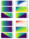 |
Fig. 1. First 1000 time steps for large simulation. Six top panels: Simulation variables for simulation with wave heating. As in the following figures, the six panels consist of density ρ, velocity V, thermal energy Eth, temperature T, and wave energies Wk±. Six bottom panels: Same, but with a much lower influx value of Wk− = W0/200 at the left boundary, resulting in almost no kink-wave heating. |
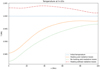 |
Fig. 2. Temperature profile as function of height at end of short simulations shown in Fig. 1 for three different simulations: one with kink-wave heating and no radiative losses, one with kink-wave heating and radiative losses, and one without kink-wave heating and radiative losses. |
The effect of the kink-wave pressure Pk is also visible in the panels of Fig. 1 showing the velocity V. The top right panel with kink wave pressure shows a gentle upflow, while the bottom panels show a gradual downflow. The latter happens because of the restructuring of the plasma due to the radiative cooling. Also visible in that panel (V of the bottom 6 panels) is the effect of the top boundary, which has a propagating signal associated with the downward kink wave, but also a signal propagating with the sound speed.
The effect of the numerical diffusivity is shown in the bottom left panel Wk+. The front of the Wk+ energy should theoretically remain a sharp interface, but it is clear that it is smoothed out during its propagation.
In Fig. 3, we show the longer duration run of the simulation with the kink-wave heating for 3100 s. In the panel with velocity V, it is shown that there is a gradual upflow generated by the kink-wave driving, of the order of 5 − 10 km/s. However, at times later than 2000 s and height above 70 Mm, numerical instabilities can be seen, which eventually crash the simulation. Some additional viscosity terms might damp out the instabilities. Still, the panel clearly shows that upflows are driven by the kink-wave pressure, because these upflows are absent in the non-driven simulation.
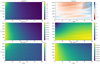 |
Fig. 3. Continuation of simulation with kink-wave heating and radiative losses until a time of 3100 s. |
As can be seen in the temperature panel, T, the temperature gradually decreases. However, it does not decrease as much as expected without wave heating. The cooling times in the simulation, calculated as τ = Eth/ℒ are from 2700 − 20 000 s. In the panel, it is clearly visible that the plasma is not cooling down as much as expected from these cooling timescales, given that the temperature’s minimum value is 0.45MK > T0/e. Thus, the kink waves are indeed partially heating the plasma, or at least sustaining it against radiative losses (similar to what was shown by Shi et al. 2021).
The cooling by the radiative losses is not entirely counteracted, and this is shown by the strong decrease in the initial temperature. As a result of the steady cooling, the plasma is restructured to fit with the new quasi-equilibrium. That leads to a drainage of density towards the footpoint, as is visible in the top left panel.
It is clear that this simulation is not the final simulation needed to conclude the UAWSOM model and determine its usefulness. Further work is needed, particularly for varying equilibrium parameters and driving parameters. It was not our aim to obtain a steady solution for the solar atmosphere, but rather a proof of concept for the application of the UAWSOM equations (Eqs. (63)–(68)).
7. Conclusions
In this work, we employed the formalism of Q variables. This formalism gives equations co-propagating with a specific wave. We used the equations of Van Doorsselaere et al. (2024) and recast the equations to an energy-propagation equation. We find that all waves show self-damping through non-linear effects, except for Alfvén waves. This is visible in the energy equation (Eq. (33)) because of terms proportional to Δα2, a parameter that is always non-zero, except in the case of Alfvén waves.
We further focused the energy-propagation equation for the case of kink waves. To that end, we followed the approach of Van Doorsselaere et al. (2020b) and averaged out the wave energy equation over the cross-section of the plume. From that averaging process, we found a single equation for kink-wave-energy evolution (Eq. (53)). This equation introduced the L⊥, VD factor, but unlike Alfvén-wave turbulence this parameter is given in terms of background properties. We find that the energy-dissipation term is proportional to (Wk±)3/2.
Such a proportionality of the damping term was also previously proposed by Zank et al. (1996). However, in his case, the damping term was multiplied by the f(σc) (which becomes zero if cross-helicity σc = ±1; i.e. only one of the counter-propagating waves). Here, on the other hand, the f(σc) remains non-zero even if only one of the propagation directions is present. Such a case was observationally considered by Adhikari et al. (2023). The presence of this term in the equation shows that kink waves (or any other wave, except for Alfvén waves) will damp even if a wave is propagating in only one direction.
Subsequently, we combined the energy-propagation equation for kink waves (Eq. (53)), with a slowly varying (in the WKB sense) background that is governed by the MHD equations. The resulting system (Eqs. (63)–(68), which we dub the UAWSOM system) has the traditional conservation of mass, momentum, and energy, but it is supplemented by wave-energy equations. The latter wave-energy equations keep track of the wave energy and the wave damping. The wave energy is then added to the total energy and incorporated in the energy-conservation equation. This ensures that energy loss of the wave results in the increase of thermal energy and thus heating of the plasma.
For now, we consider this system of equations to be an extension to the classical AWSOM model of van der Holst et al. (2014). On top of the AWSOM model, we additionally incorporated the kink-wave driving. The kink-wave-evolution equation is apparently very similar to the Alfvén-wave-evolution equation. However, the difference is in the damping term. The Alfvén waves require counter-propagating waves to initiate the cascade to turbulent heating, and low in the atmosphere the reflected waves are not strong enough to generate sufficient heating. The damping term for the kink waves, however, also operates when there is no counter-propagating wave. Thus, the kink waves can already start heating the plasma low down in the atmosphere where the damping is further enhanced by the large density gradients of the flux tubes (and despite the absence of reflected waves). It may thus be that kink waves play a key role in providing the jump start to solar-coronal and solar-wind heating low down in (say) the first few hundred megametres.
In principle, the formalism for the addition of a kink-wave equation can also be used to incorporate a third equation on the slow wave driving and development. That would allow us to model the interaction of the parametric instability and its influence on the reflection of the Alfvén waves. We would thus be able to capture the essential physics in the Shoda et al. (2019) paper in a similar 1D model. This is left for a future work.
Lastly, we implemented the UAWSOM equations in a Python module, where we considered the 1D version of the full set of equations (Eqs. (63)–(68), albeit with the Alfvén-wave power set to 0). We show that the kink-wave driving of the solar atmosphere leads to the generation of upflows. Moreover, the uniturbulent damping of the kink waves leads to the heating of the plasma, which seems most significant in the low corona. In some regions in our simulation, the kink-wave heating was able sustain the plasma against the cooling by radiative losses, but in others it was not. These initial results with the Python implementation show that further work is needed, but it also showcases the potential that the UAWSOM model holds. As such, the implementation offered in this article serves as a proof-of-concept rather than a full investigation of this model’s usefulness.
In a future work, we will compare 1D and 3D solar atmospheres driven solely by Alfvén waves, by kink waves, and by mixed models (with varying ratios of kink- and Alfvén-wave energy content). The comparison of these models to observations will allow us to place bounds on the ratio of kink-wave- and Alfvén-wave-driving energy.
Acknowledgments
TVD was supported by the European Research Council (ERC) under the European Union’s Horizon 2020 research and innovation programme (grant agreement No 724326), the C1 grant TRACEspace of Internal Funds KU Leuven, and a Senior Research Project (G088021N) of the FWO Vlaanderen. Furthermore, TVD received financial support from the Flemish Government under the long-term structural Methusalem funding program, project SOUL: Stellar evolution in full glory, grant METH/24/012 at KU Leuven. The research that led to these results was subsidised by the Belgian Federal Science Policy Office through the contract B2/223/P1/CLOSE-UP. It is also part of the DynaSun project and has thus received funding under the Horizon Europe programme of the European Union under grant agreement (no. 101131534). Views and opinions expressed are however those of the author(s) only and do not necessarily reflect those of the European Union and therefore the European Union cannot be held responsible for them. TVD is grateful for the hospitality of Iñigo Arregui (IAC, Tenerife) where these results were discussed. NM acknowledges Research Foundation – Flanders (FWO Vlaanderen) for their support through a Postdoctoral Fellowship. MVS acknowledge support from the French Research Agency grant ANR STORMGENESIS #ANR-22-CE31-0013-01. This research was supported by the International Space Science Institute (ISSI) in Bern, through ISSI International Team project #560.
References
- Adhikari, L., Zank, G. P., Telloni, D., Zhao, L. L., & Pitna, A. 2023, J. Phys. Conf. Ser., 2544, 012007 [Google Scholar]
- Alvarado-Gómez, J. D., Cohen, O., Drake, J. J., et al. 2022, ApJ, 928, 147 [CrossRef] [Google Scholar]
- Anfinogentov, S., Nakariakov, V. M., Mathioudakis, M., Van Doorsselaere, T., & Kowalski, A. F. 2013, ApJ, 773, 156 [Google Scholar]
- Anfinogentov, S. A., Nakariakov, V. M., & Nisticò, G. 2015, A&A, 583, A136 [NASA ADS] [CrossRef] [EDP Sciences] [Google Scholar]
- Antolin, P., & Van Doorsselaere, T. 2019, Front. Phys., 7, 85 [Google Scholar]
- Banerjee, D., Teriaca, L., Doyle, J. G., & Wilhelm, K. 1998, A&A, 339, 208 [Google Scholar]
- Bruno, R., & Carbone, V. 2013, Liv. Rev. Sol. Phys., 10, 2 [Google Scholar]
- Cohen, O., Glocer, A., Garraffo, C., et al. 2024, ApJ, 962, 157 [NASA ADS] [CrossRef] [Google Scholar]
- De Moortel, I., & Howson, T. A. 2022, ApJ, 941, 85 [NASA ADS] [CrossRef] [Google Scholar]
- De Pontieu, B., Carlsson, M., Rouppe van der Voort, L. H. M., et al. 2012, ApJ, 752, L12 [Google Scholar]
- Dere, K. P., Landi, E., Young, P. R., et al. 2009, A&A, 498, 915 [NASA ADS] [CrossRef] [EDP Sciences] [Google Scholar]
- Downs, C., Lionello, R., Mikić, Z., Linker, J. A., & Velli, M. 2016, ApJ, 832, 180 [Google Scholar]
- Evans, R. M., Opher, M., Oran, R., et al. 2012, ApJ, 756, 155 [NASA ADS] [CrossRef] [Google Scholar]
- Evensberget, D., & Vidotto, A. A. 2024, MNRAS, 529, L140 [Google Scholar]
- Gao, Y., Tian, H., Van Doorsselaere, T., & Chen, Y. 2022, ApJ, 930, 55 [NASA ADS] [CrossRef] [Google Scholar]
- Goossens, M., Hollweg, J. V., & Sakurai, T. 1992, Sol. Phys., 138, 233 [Google Scholar]
- Goossens, M., Terradas, J., Andries, J., Arregui, I., & Ballester, J. L. 2009, A&A, 503, 213 [NASA ADS] [CrossRef] [EDP Sciences] [Google Scholar]
- Goossens, M., Andries, J., Soler, R., et al. 2012, ApJ, 753, 111 [Google Scholar]
- Goossens, M., Van Doorsselaere, T., Soler, R., & Verth, G. 2013, ApJ, 768, 191 [NASA ADS] [CrossRef] [Google Scholar]
- Guo, M., Van Doorsselaere, T., Karampelas, K., et al. 2019, ApJ, 870, 55 [Google Scholar]
- Guyer, J. E., Wheeler, D., & Warren, J. A. 2009, Comput. Sci. Eng., 11, 6 [NASA ADS] [CrossRef] [Google Scholar]
- Hahn, M., & Savin, D. W. 2013, ApJ, 776, 78 [NASA ADS] [CrossRef] [Google Scholar]
- Hermans, J., & Keppens, R. 2021, A&A, 655, A36 [NASA ADS] [CrossRef] [EDP Sciences] [Google Scholar]
- Hillier, A., Barker, A., Arregui, I., & Latter, H. 2019, MNRAS, 482, 1143 [Google Scholar]
- Ismayilli, R., Van Doorsselaere, T., Goossens, M., & Magyar, N. 2022, Front. Astron. Space Sci., 8, 241 [NASA ADS] [CrossRef] [Google Scholar]
- Ismayilli, R., Van Doorsselaere, T., Magyar, N., Changmai, M., & Verdini, A. 2024, Phys. Fluids, 36, 065109 [Google Scholar]
- Karampelas, K., & Van Doorsselaere, T. 2018, A&A, 610, L9 [NASA ADS] [CrossRef] [EDP Sciences] [Google Scholar]
- Karampelas, K., & Van Doorsselaere, T. 2021, ApJ, 908, L7 [NASA ADS] [CrossRef] [Google Scholar]
- Lim, D., Van Doorsselaere, T., Berghmans, D., et al. 2023, ApJ, 952, L15 [NASA ADS] [CrossRef] [Google Scholar]
- Magyar, N., & Nakariakov, V. M. 2021, ApJ, 907, 55 [NASA ADS] [CrossRef] [Google Scholar]
- Magyar, N., Van Doorsselaere, T., & Goossens, M. 2017, Nat. Sci. Rep., 7 [Google Scholar]
- Magyar, N., Van Doorsselaere, T., & Goossens, M. 2019, ApJ, 882, 50 [Google Scholar]
- Morton, R. J., Tiwari, A. K., Van Doorsselaere, T., & McLaughlin, J. A. 2021, ApJ, 923, 225 [NASA ADS] [CrossRef] [Google Scholar]
- Nakariakov, V. M., Zhong, S., Kolotkov, D. Y., et al. 2024, Rev. Mod. Plasma Phys., 8, 19 [NASA ADS] [CrossRef] [Google Scholar]
- Nechaeva, A., Zimovets, I. V., Nakariakov, V. M., & Goddard, C. R. 2019, ApJS, 241, 31 [NASA ADS] [CrossRef] [Google Scholar]
- Nisticò, G., Nakariakov, V. M., & Verwichte, E. 2013, A&A, 552, A57 [NASA ADS] [CrossRef] [EDP Sciences] [Google Scholar]
- Pant, V., & Van Doorsselaere, T. 2020, ApJ, 899, 1 [NASA ADS] [CrossRef] [Google Scholar]
- Parashar, T. N., Goldstein, M. L., Maruca, B. A., et al. 2020, ApJS, 246, 58 [Google Scholar]
- Pelouze, G., Van Doorsselaere, T., Karampelas, K., Riedl, J. M., & Duckenfield, T. 2023, A&A, 672, A105 [NASA ADS] [CrossRef] [EDP Sciences] [Google Scholar]
- Petrova, E., Magyar, N., Van Doorsselaere, T., & Berghmans, D. 2023, ApJ, 946, 36 [CrossRef] [Google Scholar]
- Petrova, E., Van Doorsselaere, T., Berghmans, D., et al. 2024, A&A, 687, A13 [NASA ADS] [CrossRef] [EDP Sciences] [Google Scholar]
- Réville, V., Velli, M., Panasenco, O., et al. 2020, ApJS, 246, 24 [Google Scholar]
- Riley, P., Downs, C., Linker, J. A., et al. 2019, ApJ, 874, L15 [Google Scholar]
- Sharma, R., & Morton, R. J. 2023, Nat. Astron., 7, 1301 [CrossRef] [Google Scholar]
- Shetye, J., Verwichte, E., Stangalini, M., & Doyle, J. G. 2021, ApJ, 921, 30 [Google Scholar]
- Shi, M., Van Doorsselaere, T., Guo, M., et al. 2021, ApJ, 908, 233 [Google Scholar]
- Shoda, M., Suzuki, T. K., Asgari-Targhi, M., & Yokoyama, T. 2019, ApJ, 880, L2 [Google Scholar]
- Shrivastav, A. K., Pant, V., Berghmans, D., et al. 2024, A&A, 685, A36 [NASA ADS] [CrossRef] [EDP Sciences] [Google Scholar]
- Sishtla, C. P., Pomoell, J., Kilpua, E., et al. 2022, A&A, 661, A58 [NASA ADS] [CrossRef] [EDP Sciences] [Google Scholar]
- Suzuki, T. K., & Inutsuka, S.-I. 2005, ApJ, 632, L49 [NASA ADS] [CrossRef] [Google Scholar]
- Terradas, J., Andries, J., Goossens, M., et al. 2008, ApJ, 687, L115 [Google Scholar]
- Thurgood, J. O., Morton, R. J., & McLaughlin, J. A. 2014, ApJ, 790, L2 [Google Scholar]
- Tian, H., McIntosh, S. W., Wang, T., et al. 2012, ApJ, 759, 144 [Google Scholar]
- Tiwari, A. K., Morton, R. J., & McLaughlin, J. A. 2021, ApJ, 919, 74 [NASA ADS] [CrossRef] [Google Scholar]
- Tomczyk, S., & McIntosh, S. W. 2009, ApJ, 697, 1384 [Google Scholar]
- Tomczyk, S., McIntosh, S. W., Keil, S. L., et al. 2007, Science, 317, 1192 [Google Scholar]
- van der Holst, B., Sokolov, I. V., Meng, X., et al. 2014, ApJ, 782, 81 [Google Scholar]
- Van Doorsselaere, T., Nakariakov, V. M., & Verwichte, E. 2008, ApJ, 676, L73 [Google Scholar]
- Van Doorsselaere, T., Gijsen, S. E., Andries, J., & Verth, G. 2014, ApJ, 795, 18 [NASA ADS] [CrossRef] [Google Scholar]
- Van Doorsselaere, T., Srivastava, A. K., Antolin, P., et al. 2020a, Space Sci. Rev., 216, 140 [Google Scholar]
- Van Doorsselaere, T., Li, B., Goossens, M., Hnat, B., & Magyar, N. 2020b, ApJ, 899, 100 [NASA ADS] [CrossRef] [Google Scholar]
- Van Doorsselaere, T., Magyar, N., Sieyra, M. V., & Goossens, M. 2024, J. Plasma Phys., 90, 905900113 [Google Scholar]
- Velli, M., Grappin, R., & Mangeney, A. 1989, Phys. Rev. Lett., 63, 1807 [Google Scholar]
- Verdini, A., Velli, M., & Buchlin, E. 2009, ApJ, 700, L39 [NASA ADS] [CrossRef] [Google Scholar]
- Verdini, A., Velli, M., Matthaeus, W. H., Oughton, S., & Dmitruk, P. 2010, ApJ, 708, L116 [Google Scholar]
- Wang, T., Ofman, L., Davila, J. M., & Su, Y. 2012, ApJ, 751, L27 [Google Scholar]
- Zank, G. P., Matthaeus, W. H., & Smith, C. W. 1996, J. Geophys. Res., 101, 17093 [Google Scholar]
- Zank, G. P., Dosch, A., Hunana, P., et al. 2012, ApJ, 745, 35 [Google Scholar]
Appendix A: Relation between wave energy w and Q density W
We have previously introduced the wave energy density in Eq. 13, which we repeat here for convenience:
We had also introduced the Q-density W± in Eq. 28:

These two expressions apparently do not coincide. In this section we explore the interrelation between these two expressions. To calculate the Q density, we start from Eqs. 7-11 to obtain
 (A.1)
(A.1)
 (A.2)
(A.2)
As discussed in Van Doorsselaere et al. (2024), we compute α in order to describe the wave in the co-moving wave frame. Thus, we have that
 (A.3)
(A.3)
We thus find that (for example) the positive, downward wave energy is
 (A.4)
(A.4)
and W− = 0. Indeed, the downward propagating wave is solely described by δQ⊥+. Now, we take the cross-sectional and wavelength average of the Q density ⟨W±⟩, where the radial integral is taken for the volume (r ∈ [0, γR]) in which this plume is the dominant structure (Van Doorsselaere et al. 2014). We relate this outer boundary γR to the filling factor f of the corona through the relation of Van Doorsselaere et al. (2014):
 (A.5)
(A.5)
Using a similar procedure as Van Doorsselaere et al. (2014) and Van Doorsselaere et al. (2024), we have as cross-sectionally averaged Q-density ⟨W±⟩ (see Eq. 43):
 (A.6)
(A.6)
 (A.7)
(A.7)
 (A.8)
(A.8)
In the second line, we have used the dispersion relation for the kink wave with ρi(Ω2 − ωAi2) = ρe(Ω2 − ωAe2), and in the third line we have used the expression for the wave amplitude Υ (see Eq. 5). The term without f corresponds exactly to the expression of the energy density ⟨w⟩ (see e.g. Eq. 10 in Van Doorsselaere et al. 2014). There is only a difference in the term proportional to the filling factor f. Note that if there are no other structures in the corona, we would integrate until r → ∞ and consequently f = 0, and hence the expression of the energy density ⟨w⟩ is in that case the same as ⟨W±⟩.
To explain this (seemingly remarkable) coincidence between the expressions for ⟨W±⟩ and ⟨w⟩, we start again from the expression for the wave energy density w (see Eq. 13) and the Q density (Eq. 28):
 (A.9)
(A.9)
 (A.10)
The equations are seemingly different, but this difference is only apparent indeed. By construction, we have that
 (A.11)
for the oppositely propagating wave. Thus, we must have
 (A.12)
Then, we see that the Q density equals
 (A.13)
This is equal to the wave energy w in case of equipartition of the wave (over the domain in which the wave energy is averaged). Thus, for well-behaved waves (such as the kink wave, which has equipartition, Goossens et al. 2013), the Q density is exactly equal to the wave energy density. As explained in Goossens et al. (2013), the equipartition between magnetic and kinetic energy for kink waves is only satisfied when considering the entire domain. Here however, the spatial domain is limited to a distance γR, so that the equipartition is not exact, made explicit by the presence of the term containing the filling factor f.
All Figures
|
Fig. 1. First 1000 time steps for large simulation. Six top panels: Simulation variables for simulation with wave heating. As in the following figures, the six panels consist of density ρ, velocity V, thermal energy Eth, temperature T, and wave energies Wk±. Six bottom panels: Same, but with a much lower influx value of Wk− = W0/200 at the left boundary, resulting in almost no kink-wave heating. |
| In the text | |
|
Fig. 2. Temperature profile as function of height at end of short simulations shown in Fig. 1 for three different simulations: one with kink-wave heating and no radiative losses, one with kink-wave heating and radiative losses, and one without kink-wave heating and radiative losses. |
| In the text | |
|
Fig. 3. Continuation of simulation with kink-wave heating and radiative losses until a time of 3100 s. |
| In the text | |
Current usage metrics show cumulative count of Article Views (full-text article views including HTML views, PDF and ePub downloads, according to the available data) and Abstracts Views on Vision4Press platform.
Data correspond to usage on the plateform after 2015. The current usage metrics is available 48-96 hours after online publication and is updated daily on week days.
Initial download of the metrics may take a while.