© ESO 2022

1 Introduction

The Kepler, K2, and TESS missions have revealed 3673 planetary systems, and 814 of them feature multiple planets¹ (see e.g., Lissauer et al. 2011; Fabrycky et al. 2014; Weiss et al. 2018). Apart from various properties and architectures, such as the number of planets, the planetary period and radii ratios observed among them, planetary pairs and triplets seem to be evolving near (just outside) or in two-body mean-motion resonances (MMRs) and three-body Laplace-like resonances (resonant chains), respectively. In particular, five out of six planets of TOI-178 are in the 2:4:6:9:12 resonant chain (Leleu et al. 2021), four planets of the HR 8799 are in the 8:4:2:1 chain (Goździewski & Migaszewski 2020), four planets of the system K2-32 evolve near the 1:2:5:7 resonant chain (Heller et al. 2019), four planets of the system Kepler-223 are in the 3:4:6:8 resonant chain (Mills et al. 2016), while five planets of the K2-138 are in the 3/2 MMR (Christiansen et al. 2018). Other examples include the multiple-planet systems Trappist-1 (Gillon et al. 2017), Kepler-18 (Cochran et al. 2011), Kepler-30 (Panichi et al. 2018), Kepler-47 (Orosz et al. 2019), Kepler-60 (Goździewski et al. 2016), and Kepler-82 (Freudenthal et al. 2019).

Recent studies have been devoted to the formation history and dynamical evolution of multiple-planet systems that yield exoplanets locked in or close to a resonant chain (e.g., Morrison et al. 2020; Pichierri & Morbidelli 2020). Lissauer & Gavino (2021) numerically analyzed the long-term orbital stability of three-planet systems where the planetary longitudes and orbital separation vary, while Siegel & Fabrycky (2021) performed a numerical exploration of equillibria dependent on the libration of the three-body resonant angles for chains consisting of first-order MMRs. Furthermore, Tamayo et al. (2021) provided a stability estimator that distinguishes quickly the unstable from the stable planetary configurations among estimated orbital parameters and masses of multiple-planet systems. Charalambous et al. (2018) chose different planetary masses and illustrated maps with stable and unstable domains of three-planet systems at which the mean-motion ratios of the planets were altered, while Petit (2021) analytically approximated first-order resonant chains of three massive planet systems with an averaged Hamiltonian.

Planetary masses and eccentricities can be precisely extracted by the transit-timing variation (TTV) method for exoplanets close to an MMR. However, employing numerical analyses or N-body simulation algorithms in order to reject orbital parameters that lead to instability events (and which cannot be estimated by observations) may become computationally expensive and time-consuming. Additionally, the published observational data often possess very large deviations that render the system chaotic in nature. Instead, by spotting the stable periodic orbits close to the exoplanetary system (for a given MMR or resonant chain, planetary masses and eccentricity values) can immediately unravel the regions where the stability is guaranteed for long-time spans. Hence, the boundaries for all the orbital elements, even the longitudes of pericenter and mean anomalies, can be delineated as the dynamical phase space of resonant exoplanets is crystallized.

Hadjidemetriou & Michalodimitrakis (1981) computed the first stable periodic orbits in the planar General 4-Body Problem (G4BP; see e.g. Hadjidemetriou 1977; Michalodimitrakis & Grigorelis 1989) for the Galilean satellites of Jupiter in the 1:2:4 resonant chain. Following their work, we apply this methodology to the exoplanets. Here, we focus on the system Kepler-51 and aim to provide hints and constraints that favor its survival. We study the dynamics and long-term stability of the system via the families of periodic orbits in the planar G4BP and extend our methodology for pairs of resonant massive exoplanets in mutually inclined orbits (Antoniadou & Voyatzis 2013, 2014) and coplanar orbits (Antoniadou 2016; Antoniadou & Voyatzis 2016) to the case of triplets of massive coplanar exoplanets in resonant chains (G4BP).

Our work is organized as follows. In Sect. 2, we provide the key points and tools employed to obtain our dynamical analysis. In Sect. 3, we discuss possible regions of long-term stable evolution in the dynamical vicinity of Kepler-51 based on the periodic orbits in the G4BP and conclude in Sect. 4. In Appendix A, we provide the equations of motion for three-planet systems (A.1), define the symmetric periodic orbits (A.2), and elaborate on the continuation method followed for the 1:2:3 resonant periodic orbits (A.3). In Appendix B, we provide details and examples on the linear stability of the periodic orbits in the G4BP (B.1) and the chaotic indicator used (B.2).

2 Main aspects of the methodology

We considered three massive planets revolving around a star on coplanar orbits. When viewed in an inertial frame of reference², these orbits correspond to Keplerian ellipses with heliocentric osculating elements, namely, the semimajor axes, a_i, the eccentricities, e_i, the longitudes of pericenter, ${\varpi }_i$, and the mean anomalies, M_i (i = 1,2,3), where subscript 1 refers to the inner planet. In computations, we use the normalized set of units where the semimajor axis of the inner planet is equal to 1, G × m_total = 1, and, subsequently, the period of the inner planet is equal to about 2π.

We chose the relative frequencies, ω_i(i = 1,2,3), of the three planets of period $T_i=\frac{2\pi }{{\omega }_i}\left(i=1,2,3\right)$ in the inertial frame, so that they be commensurable as follows: $$\frac{{\omega }_2-{\omega }_1}{{\omega }_3-{\omega }_1}\approx \frac{P}{Q},$$(1)

where P, Q ∈ ℤ*.

Then, in the rotating frame of reference we can define the relative period, T, of a system where planet 2 with period T₂ revolves P times about planet 1 with period T₁, while planet 3 with period T₃ revolves Q times around planet 1, that is: $$T\approx \frac{T_1}{1-\frac{T_1}{T_2}}P\approx \frac{T_1}{1-\frac{T_1}{T_3}}Q.$$(2)

Certain orbits that fulfill a specific periodicity condition in the rotating frame are called symmetric periodic orbits (see Appendix A.2 for more details). These periodic orbits correspond to the exact location of the MMR. In this work, we focus exclusively on the symmetric elliptic (resonant) periodic orbits, which have ${\varpi }_i$ = 0 or π (i = 1,2,3)³.

Described within another context, the periodic orbits are the fixed (or periodic) points of a Poincaré map and correspond also to the fixed points (or stationary solutions) of an averaged Hamiltonian, as long as the latter is accurate enough. Following the continuation schemes explained in Appendices A.2 and A.3, these points form the so-called characteristic curves or families of periodic orbits.

The periodic orbits depend on the resonant angles, θ_i (i = 1,…, 4), which, given the 1:2:3 resonant chain studied, take the following form: $$\begin{array}{lll}{\theta }_1\hfill & =\hfill & 2{\lambda }_2-{\lambda }_1-{\varpi }_1,\hfill \\ {\theta }_2\hfill & =\hfill & 2{\lambda }_2-{\lambda }_1-{\varpi }_2,\hfill \\ {\theta }_3\hfill & =\hfill & 3{\lambda }_3-{\lambda }_2-{\varpi }_3,\hfill \\ {\theta }_4\hfill & =\hfill & 3{\lambda }_3-{\lambda }_2-{\varpi }_2,\hfill \\ {\varphi }_{\text{L}}\hfill & =\hfill & {\theta }_4-{\theta }_2=3{\lambda }_3-4{\lambda }_2+{\lambda }_1,\hfill \end{array}$$(3)

with ${\lambda }_i={\varpi }_i+M_i$ as the mean longitude, $\Delta {\varpi }_{21}={\varpi }_2-{\varpi }_1$ and $\Delta {\varpi }_{32}={\varpi }_3-{\varpi }_2$ as the apsidal differences, and with ø_L as the Laplace angle.

If the periodic orbit is symmetric, the angles in Eq. (3) are equal to either 0 or π. In order to distinguish the families of periodic orbits that belong to different configurations, we present them on the (e₁ cos θ₁, e₂ cos θ₂) and (e₂ cos θ₂, e₃ cos θ₃) planes.

The characteristic curves of the families change significantly, when the mass-ratio changes (see e.g. Antoniadou & Voyatzis 2013) for the 2/1 MMR and (see e.g. Antoniadou & Voyatzis 2014) for the 4/3, 3/2, 5/2, 3/1 and 4/1 MMRs. If the mass values change, but still retain the same order of magnitude and preserve their ratio, then the main properties of the families (location and stability) do not show significant variations (see e.g. Voyatzis 2008). Therefore, in order to distinguish the families that belong to the same configuration but have been computed for different mass-ratios, we introduce two planetary mass-ratios; one for the innermost and one for the outermost pair, namely, ${\rho }_i=\frac{m_c}{m_b}$ and ${\rho }_o=\frac{m_d}{m_c}$ respectively.

It is widely known in Hamiltonian systems that stable periodic orbits are surrounded by invariant tori where the motion is regular and quasi-periodic, whereas the neighborhood of unstable periodic orbits can give rise to instability events (either weak chaos or strong chaos with collisions or escapes). In the neighborhood of stable periodic orbits, all the resonant angles librate, while all or some of them exhibit rotation in the vicinity of the unstable ones.

The libration of all the resonant angles θ_i (i = 1,…, 4) signifies a two-body MMR (hereafter denoted as R_L), where $\frac{n_2}{n_1}={\left(\frac{a_1}{a_2}\right)}^{-3/2}\approx \frac{p_1+q_1}{p_1}\text{and}\frac{n_3}{n_2}={\left(\frac{a_2}{a_3}\right)}^{-3/2}\approx \frac{p_2+q_2}{p_2}$ with p_i,q_i ∈ ℤ*. and qi being the order of the MMR, implying that the libration of the Laplace angle, ø_L, is simply the consequence of the two independent MMRs which overlap. However, ø_L can librate while the rest of the resonant angles, θ_i, rotate. The latter indicates a state where the pairs of planets are not locked in a two-body MMR, but the triplet is locked in a three-body resonance (resonant chain, denoted as R_T), where ${\left(\frac{n_2}{n_3}\right)}^{-1}\approx \frac{p+q-s}{q}-\frac{p}{q}\left(\frac{n_1}{n_2}\right)$ with p, q, s ∈ ℤ^* and s being the order of the resonance (see e.g., Morbidelli 2002). These resonance mechanisms provide a phase protection. Inside an MMR, we can observe a secondary resonance (denoted as R_S) or an apsidal difference oscillation (denoted as R_A). In the former case, we consider the frequency ratio between the libration frequency of θ₁ and the rotation frequency of θ₂ (see e.g., Lemaitre & Henrard 1990), while in the latter case, only the apsidal difference oscillates and the rest of the angles rotate. At the non-resonant low-eccentricity orbits, an apsidal resonance, where only the apsidal difference librates, may become apparent. In the following, we also use a notation of R with two subscripts, namely R_i,o, in order to denote two separate behaviors of the inner and outer pairs of planets. For instance, the combination of a secondary resonance of the inner pair with either an MMR or an apsidal difference oscillation of the outer pair is denoted as R_s,l or R_SA, respectively. The above dynamical mechanisms have been extensively showcased in the neighborhood of periodic orbits by Antoniadou & Libert (2018, for the minor-body dynamics) and are all observed in the regular domains in phase space, where even massive planets can evolve in a stable way (Antoniadou & Voyatzis 2016).

We study the long-term orbital stability of three-planet systems based on two methods: (i) linear stability of the periodic orbits (explained in Appendix B.1) and (ii) maps of dynamical stability (DS-maps) by computing the chaotic indicator DFLI (see Appendix B.2). The first method yields either stable or unstable periodic orbits, which are either colored blue or red along the families. Based on the stable periodic orbits, we seed the second method and construct DS-maps around the (near)-resonant exoplanets and provide a visualization of the boundaries of the orbital elements securing regular motion.

3 Dynamical constraints on Kepler-51

The system Kepler-51 has been regularly studied (see e.g., Steffen et al. 2013; Hadden & Lithwick 2014,2017; Masuda 2014; Morton et al. 2016; Holczer et al. 2016; Berger et al. 2018; Gajdos et al. 2019; Libby-Roberts et al. 2020; Battley et al. 2021). Its innermost planetary pair evolves close to the 2/1 MMR, according to the period ratio $\frac{T_c}{T_b}=1.89$, while the outermost one is in the 3/2 MMR, as $\frac{T_d}{T_c}=1.53$ In what follows, we present the families of periodic orbits in the 1:2:3 resonant chain and construct DS-maps that unveil the dynamical vicinity of Kepler-51 in order to explore the dynamical mechanisms that may guarantee its orbital stability.

3.1 Families of symmetric periodic orbits for Kepler-51

Following the continuation method illustrated in Appendix A.2, we set P = 3 and Q = 4 in Eq. (A.12), which for k=4, yield the following: $$\left(\frac{T_2}{T_1},\frac{T_3}{T_1},\frac{T_3}{T_2}\right)=\left(\frac{2}{1},\frac{3}{1},\frac{3}{2}\right),$$(4)

namely, the resonant chain of the 2/1 and 3/2 MMRs is established for the innermost and outermost pairs of Kepler-51.

We then take into account the planetary eccentricity values of Kepler-51 (shown in Table 2). In Fig. 1, we present the six groups of families of planar symmetric periodic orbits, S_i (i=1…6), in the 1:2:3 resonant chain, which reside very close to these observational values on the (e₁, e₂) and (e₂, e₃) planes. Each of these six groups consists of families of the same configuration (shown in Table 3), but has different planetary mass-ratios, namely, ${\rho }_i=\frac{m_c}{m_b}$ and ${\rho }_o=\frac{m_d}{m_c}$ (shown in Table 1). Each planetary-mass ratio is identified by a number on each panel. More particularly, label 1 corresponds to Masuda (2014), label 2 to Libby-Roberts et al. (2020), label 3 to default, and label 4 to high-mass priors considered by Battley et al. (2021).

We observe that the segments of stable periodic orbits are not altered in their extent since the considered planetary mass-ratios vary, even though the reflection of the four different sets of planetary masses (shown in Table 1) on the mass-ratios seems quite important and widely ranging; for instance, from 1.2 (Libby-Roberts et al. 2020) to 2.57 (Battley et al. 2021). When the dynamics is being studied, apart from the masses themselves, one major factor that affects it is the order of the mass values. More precisely, the divergence of the families and their stability segments as the mass-ratios vary are affected differently for giant Jovian planets and terrestrial ones; and all studies performed for the super-puff planets of Kepler-51 attribute masses of the same order (10^–6–10^–5).

Since the change on the dynamics is not significant among the various planetary masses considered in Table 1, in what follows, we chose to focus on the study of Masuda (2014). Our choice is also justified by both Battley et al. (2021) and Libby-Roberts et al. (2020) who conclude that their mass values are less constrained and not improved when compared to Masuda (2014).

In the top panels of Fig. 2, six families of planar periodic orbits, S_i (i = 1…6), in the 1:2:3 resonant chain are presented on the signed-eccentricity planes. In the bottom panels, we provide all (nine) families up to high-eccentricity values, even though only low-eccentricity stable periodic orbits were found. The families were computed for the planetary masses of Kepler-51, shown in Table 2. In Table 3, we provide the longitudes of pericenter, mean anomalies and resonant angles along each family together with the eccentricity values at which a transition of the configuration takes place. Given the observational values of the eccentricities (see Table 2), depicted by a cyan “+” symbol, along with their deviations (shown as magenta dashed lines), we focus on the low-eccentricity regime (top panels).

More precisely, solely the families S₁, S₄, S₅ and S₆ possess stable (blue colored) periodic orbits. These are found in the configurations (θ₁,θ₂,θ₃,θ₄) = (0,π, 0,π) and (O,π,π,π) for the S₁ family; (π, 0,0,0) for the S₄ family; (π, π, 0, π) for the S₅ family; and (0, π, π, 0) for the S₆ family.

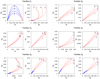Fig. 1 Groups of families, Si (i = 1…6), of planar symmetric periodic orbits in the 1:2:3 resonant chain with stable segments close to the dynamical vicinity of Kepler-51 presented on the (e1, e2) and (e2, e3) planes. Each of these six groups consists of families of the same configuration (shown in Table 3), but with different planetary mass-ratios, that is, ${\rho }_i=\frac{m_c}{m_d}\text{and}{\rho }_o=\frac{m_c}{m_d}$ (shown in Table 1 and labeled from 1 to 4 on each panel). Label 1 corresponds to Masuda (2014), label 2 to Libby-Roberts et al. (2020), label 3 to default, and label 4 to high-mass priors considered by Battley et al. (2021). The stable (unstable) periodic orbits are depicted by blue (red) solid curves.

3.2 DS-maps and constraints for Kepler-51

Discerning distinct regions of regular and chaotic motion in phase space can sometimes be demanding for Hamiltonian systems of 5 degrees of freedom (planar G4BP). The use of chaotic indicators can assist in deciphering such domains. However, all indicators have their pros and cons (see e.g., Maffione et al. 2011, for a comparison between the Lyapunov Indicator (LI), the Mean Exponential Growth factor of Nearby Orbits (MEGNO), the Smaller Alignment Index (SALI), the FLI, and the Relative Lyapunov Indicator (RLI)). In this paper, we use a version of the FLI (called DFLI; see Appendix B.2 for its definition). Concerning dynamical systems such as the planetary ones, the DFLI was established as efficient and reliable by Voyatzis (2008).

With regard to the computation of the DS-maps, we constructed 100 × 100 grid planes and focused on the S₁, S₅, and S₆ families, namely, we chose specific orbital elements from the symmetric periodic orbits that belong to these families (their angles are reported in Table 3), since their stable segments are closer to the observational eccentricity values of Kepler-51. We remind the reader that the chosen families of periodic orbits have been computed for the masses of Kepler-51 (identified by label 1; i.e., Masuda (2014) in Fig. 1 and shown in their full extent in (Fig. 2) and for the 1:2:3 resonant chain. We note also that the values of the semimajor axes vary slightly along the families, but the resonance remains almost constant (see Appendix A.3 for the differences between these elliptic S_i families and the circular family along which the resonance varies). More precisely, on each grid plane, we vary a pair of the orbital elements, while keeping the rest of the orbital elements and masses of the periodic orbit fixed. In the following, we mention the orbital elements of the selected periodic orbits used for the construction of each DS-map and justify their selection.

In order to classify the orbits, we chose a maximum integration time for the computation of the DFLI equal to t_max = 3 Myr, which corresponds approximately to 24 million orbits of the innermost planet, b, or 8.5 million orbits of the outermost planet, d, and was deemed appropriate, in order to distinguish chaos from order reliably for the particular application. We used the Bulirsch–Stoer integrator with a tolerance of 10^–14. For small values of DFLI (dark-colored domains), a regular evolution for the planets is expected. In our study, we halt the integrations either when DFLI(t) > 30 or when t_max is reached.

In Fig. 3, we present DS-maps on the planes (e₁, e₂) and (e₂, e₃) in the top panels and (∆ϖ₂₁, ∆M₂₁) and (∆ϖ₃₂, ∆M₃₂) in the bottom panels. The rest of the orbital elements that remain fixed for each of the initial conditions on the DS-maps are chosen from the planar periodic orbit in the S6 family, with values for e2 and e3 that coincide approximately with the observational eccentricities, namely, e_c and e_d (depicted by the magenta “+” symbol in the top right panel), respectively. The selected periodic orbit has the following orbital elements: a₁ = 1.04268089, a₂ = 1.65662643, a₃ = 2.17192389, e₁ = 0.0075847, e₂ = 0.0150072, e₃ = 0.0080335, ϖ₁ = 0°, ϖ₂ = 180°, ϖ₃ = 0°, M₁ = 0°, M₂ = 0°, and M₃ = 180°, with the following configuration: (θ₁,θ₂,θ₃,θ₄) = (0, π, π, 0).

In Fig. 4, we present DS-maps by varying the eccentricities on the planes (e₁, e₂) and (e₂, e₃). The rest of the orbital elements, which remain fixed for each of the initial conditions on the DS-maps, are selected from a planar stable (blue) periodic orbit of the S₅ family being closer to the observational values e_c and e_d (errors counted in). Its orbital elements are: a₁ = 0.99089944, a₂ = 1.56964834, a₃ = 2.05151434, e₁ = 0.0025747, e₂ = 0.0050208, e₃ = 0.0030763, ϖ₁ = 180°, ϖ₂ = 180°, ϖ₃ = 0°, M₁ = 180°, M₂ = 180°, and M₃ = 0°, which correspond to the following configuration: (θ₁,θ₂,θ₃,θ₄) = (π, π, 0, π).

Likewise, in Fig. 5, we present DS-maps by varying the eccentricities on the planes (e₁, e₂) and (e₂, e₃). The rest of the orbital elements, which remain fixed for each of the initial conditions on the DS-maps, are selected from a planar stable periodic orbit of the S₁ family, where e₁ ≈ e_b. Its orbital elements are: a₁ = 1.02641224, a₂ = 1.62959097, a₃ = 2.13398349, e₁ = 0.0400329, e₂ = 0.0030374, e₃ = 0.0000763, ϖ₁ = 0°, ϖ₂ = 180°, ϖ₃ = 0°, M₁ = 0°, M₂ = 180°, and M₃ = 0°, with the following configuration: (θ₁,θ₂,θ₃,θ₄) = (0, π, 0, π).

In Fig. 6, we provide the DS-maps that showcase the extent of each resonance (the 2/1 MMR in the left panels and the 3/2 MMR in the right ones) in relation to each planetary eccentricity value. We were guided by the same periodic orbit of the S₆ family that was used in Fig. 3 in the configuration (θ₁,θ₂,θ₃,θ₄) = (0,π,π, 0). The observational values of the semimajor axes and eccentricities are denoted by the magenta “+” symbol.

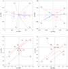Fig. 2 Families, Si (i = 1…9), of planar symmetric periodic orbits in the 1:2:3 resonant chain close to the dynamical vicinity of Kepler-51 (top panels) and until their termination points (bottom panels) presented on the (e1 cos θ1, e2 cos θ2) and (e2 cos θ2, e3 cos θ3) planes. The angles for the different configurations of the families are shown in Table 3. Kepler-51 is identified in the top panels by the cyan “+” symbol, while the errors provided by Masuda (2014) are delineated by magenta dashed lines.

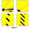Fig. 3 DS-maps on the (e1, e2) and (e2, e3) planes, where the family S6 is projected, and the (∆ϖ21, ∆M21) and (∆ϖ32, ∆M32) planes. Kepler-51 is identified by the magenta “+” symbol, while the errors are delineated by magenta dashed lines. The color bar illustrates the DFLI values; dark colors correspond to regular evolution, while pale ones signify chaoticity. RL indicates that both pairs of planets are locked in a two-body MMR (2/1 and 3/2 MMR), while RS,L indicates the 1/1 secondary resonance inside the 2/1 MMR for the inner pair and a locking in the 3/2 MMR for the outer pair of planets.

3.2.1 Apsidal resonance for non-resonant low-eccentricity orbits

At the low-eccentricity non-resonant orbits presented in Fig. 6, that is, away from the distinct RL regions found around the values $\frac{a_2}{a_1}\approx 1.58\text{and}\frac{a_3}{a_2}\approx 1.31$, an apsidal resonance is found at the position of Kepler-51. In such an evolution (shown in Fig. 7), all the resonant angles rotate, but the apsidal differences librate about π, given the configuration (θ₁, θ₂, θ₃, θ₄) = (0, π, π, 0) of the periodic orbit from the S₆ family used.

3.2.2 Two-body MMRs, R_L

The dynamical mechanism of two independent two-body MMRs, namely the 2/1 for the innermost planets and the 3/2 for the outermost ones, was encountered in the neighborhood of families S₆ and S₅ (R_L symbols on the DS-maps in Figs. 3 and 4). The evolutions of the orbital elements and the resonant angles from the initial conditions taken from these two “R_L regions” are demonstrated in the left panels of Figs. 8 and 9. In the former case, the resonant angles,(θ₁,θ₂,θ₃,θ₄), librate about (0, π, π, 0), while in the latter, the resonant angles librate about (π, π, 0, π).

Regarding the S₅ family, this mechanism is stronger the closer we get to the family, as the libration widths of the resonant MMRs in relation to each eccentricity value. The angles are very small. Therefore, we may conjecture that the two-body MMRs cannot act as a safeguard for the regular evolution of Kepler-51 when found in its dynamical vicinity.

In contrast, the S₆ family may provide a region that could host Kepler-51 for long-time spans should the pairs be in two-body MMRs. More precisely, the dark-colored regular domain on the (e₂, e₃) plane of Fig. 3 almost engulfs the observational eccentricities, ec and ed, along with their deviations. Given this overlap, a constraint should be imposed on the eccentricity eb, since the R_L region takes place when e₁ < 0.02, which is by far lower than the lowest deviation boundary (magenta dashed line) on the (e₁, e₂) plane of Fig. 3. Additionally, guided by the same stable periodic orbit, the boundaries for the mean anomalies and apsidal differences can be deduced by the bottom panels of Fig. 3.

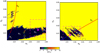Fig. 4 DS-maps on the eccentricity planes (e1, e2) and (e2, e3), where the family S5 is projected. RL denotes a two-body MMR (2/1 and 3/2 MMR for the inner and outer pairs of planets), RT indicates a three-body Laplace-like resonance (1:2:3 resonant chain), while RSA indicates the 1/1 secondary resonance inside the 2/1 MMR for the inner pair and an apsidal difference oscillation/rotation observed for the outer pair of planets. Colors and lines as in Fig. 3.

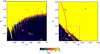Fig. 5 DS-maps on the eccentricity planes (e1, e2) and (e2, e3), where the family S1 is projected. Rs,a indicates the 1/1 secondary resonance inside the 2/1 MMR for the inner pair and an apsidal difference oscillation/rotation observed for the outer pair of planets. Colors and lines as in Fig. 3.

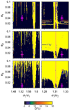Fig. 6 DS-maps that showcase the extent of the 2/1 (left panels) and the 3/2 (right panels) distinct RL regions appear at the values$\frac{a_2}{a_1}\approx 1.58\text{and}\frac{a_3}{a_2}\approx 1.31$. The magenta lines showcase the nominal values of each MMR. The system Kepler-51 (magenta dashed lines enclosing the “+” symbol) is found at $\frac{a_c}{a_b}\approx 1.527\text{and}\frac{a_d}{a_c}\approx 1.325$, where an apsidal resonance takes place. Colors and lines as in Fig. 3.

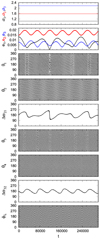Fig. 7 Evolution of the orbital elements and resonant angles along an orbit initiated by the non-resonant low-eccentricity orbits, showcasing an apsidal resonance (shown in Fig. 6).

3.2.3 Three-body Laplace-like resonance, R_T

The dynamical mechanism of a three-body Laplace-like resonance, namely, the 1:2:3 resonant chain, was encountered in the neighborhood of the S₅ family (R_T symbols in the left panel of Fig. 4). The evolution of the orbital elements and the resonant angles, with initial conditions taken from the “R_T region” within the magenta dashed lines, is shown in the right panel of Fig. 9, where the resonant angles rotate, but the Laplace angle librates about 0°.

We may cautiously impose further constraints on the observational eccentricities for the 1:2:3 resonant chain to be long-term viable, by taking into account the regular domains (dark “R_T regions”) and the overlapping deviations (magenta dashed lines). More particularly, e_c < 0.016 (deduced from the regular R_T region in the left panel of Fig. 4), while e_d < 0.006 (which is the highest value of e₃ in the stable segment of the S₅ family).

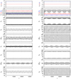Fig. 8 Evolution of the orbital elements and resonant angles along orbits initiated by the RL region (left panel) and the RS,L region (right panel) dynamically unveiled by the S6 family (shown in Fig. 3).

3.2.4 Combination of secondary resonance, two-body MMR and apsidal difference oscillation, R_S,L, and R_S,A

The dynamical mechanism of the 1/1 secondary resonance inside the 2/1 MMR for the innermost planets and a locking in the 3/2 MMR for the outermost ones, was encountered in the neighborhood of the S₆ family (R_S,L symbols in the top left panel of Fig. 3). The evolution of the orbital elements and the resonant angles, with initial conditions taken from the R_S,L region within the magenta dashed lines, is shown in the right panel of Fig. 8, where a libration is observed for θ₁ about 0°, θ₃ about 180°, θ₄ about 0° and ∆ϖ₃₂ about 180° and a rotation for the rest of angles.

The regular domain exhibiting this mechanism is particularly thin and the region delineated by the deviations of observational eccentricities (magenta dashed lines) is populated mainly by chaotic orbits. Hence, we do not put any constraints on Kepler-51 stemming from the R_S,L region dynamically unveiled by the S₆ family, since such an evolution may not be probable.

The dynamical mechanism of the 1/1 secondary resonance inside the 2/1 MMR for the innermost planets and an apsidal difference oscillation/rotation observed for the outer pair of planets, was encountered in the neighborhood of the S₅ and S₁ families (Rs,a symbols in Figs. 4 and 5). The evolution of the orbital elements and the resonant angles, with initial conditions taken from the R_S,A regions within the magenta dashed lines of Figs. 4 and 5, is shown in the left and right panels of Fig. 10, respectively. In the R_S,A region originating from the S₅ family, θ₁ librates about 180° and Δϖ₃₂ oscillates about 180°, following the configuration of the chosen periodic orbit that was used for the DS-map construction. As for the Rs,a region established by the periodic orbit of the S₁ family, θ₁ librates about 0°, while ∆ϖ₃₂ alternates between large amplitude oscillations about 0^° and circulations, revealing the chaotic nature of this motion.

Regarding the R_S,A region in the DS-map of Fig. 4, we observe that e_c and e_d along with their deviations fall mainly on the unstable (red colored) periodic orbits. Therefore, the long-term stability may be possible but not very probable within these very small regular domains.

Concerning the Rs,a region in the DS-maps of Fig. 5, we observe that eb and ec, along with their deviations, fall entirely on the regular domain. As a result, we performed a search for possible boundaries for the mean anomalies and apsidal differences guided by the same stable periodic orbit used for the DS-maps on the eccentricity planes. We found that essentially all values in the domain [0, 180] yield a regular R_S,A mechanism. However, we recall that the above values hold for eccentricity, namely, ed ≈ 0 (see the S₁ family).

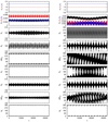Fig. 9 Evolution of the orbital elements and resonant angles along orbits initiated by the RL region (left panel) and the RT region (right panel) dynamically unveiled by the S5 family (shown in Fig. 4).

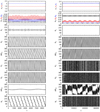Fig. 10 Evolution of the orbital elements and resonant angles along orbits initiated by the Rs,a regions dynamically unveiled by the S5 (left panel) and S1 (rightpanel) families (shown in Figs. 4 and 5, respectively).

4 Conclusions

Motivated by the increasing numberofexoplanets evolving in (or close) to MMRs and resonant chains, we analyzed the long-term orbital stability of the system Kepler-51. We presented novel results regarding the 1:2:3 resonant symmetric periodic orbits of the G4BP, which was used as a model to provide hints on the dynamics of the three planets.

For the planetary masses of Kepler-51, only four families were found to possess stable segments in the low-eccentricity dynamical neighborhood of the system. These families are in the symmetric configurations (θ₁,θ₂,θ₃,θ₄) = (0,π, 0,π) and (0,π,π,π) (S₁ family); (π, 0,0,0) (S₄ family); (π,π, 0,π) (S₅ family); and (0, π, π, 0) (S₆ family)⁴.

Guided by the stable symmetric periodic orbits of these families, we computed DS-maps, which basically unraveled the three main dynamical mechanisms which secure the long-term orbital stability of the system Kepler-51. More precisely, the 2/1 and 3/2 two-body MMRs (denoted as Rl), the 1:2:3 three-body Laplace-like resonance (denoted as R_T), and a combination of mechanisms for the inner and outer pairs separately, namely, the 1/1 secondary resonance inside the 2/1 MMR for the inner pair with either a 3/2 MMR or an apsidal difference oscillation for the outer pair (denoted as R_S,L and R_S,A, respectively).

Based on the regular domains demonstrated in the DS-maps, we put possible constraints on the observational eccentricities, mean anomalies, and apsidal differences. For the first scenario in the R_L region, we concluded that e_b < 0.02 and we presented possible islands of stability for the angles, so that such two-body MMRs endure for long time spans. For the second scenario in the R_T region, we found e_c < 0.016 and e_d < 0.006 to be viable for such a chain. For the third scenario, we deduced that an evolution comprising the 1/1 secondary resonance with a 3/2 MMR (R_S,L region) may be possible but not probable. Additionally, we showed that an evolution in an R_S,A region, despite it being of a chaotic nature, fits very well with the observational eccentricities e_b and e_c (and almost any value for the mean anomalies and the apsidal differences), as long as e_d ≈ 0.

With regard to two-planet systems, many fitting methods have been developed and dynamical analyses have been performed for giant planets locked in MMRs in tandem with migration simulations (see e.g., Hadden & Payne 2020). An efficient fitting of the observational data for systems of three planets in (or near) a resonance is beyond any question. With the aim of obtaining an optimum deduction of the orbital elements, this study exemplifies the need for dynamical analyses based on periodic orbits performed in parallel to the data fitting methods.

Acknowledgements

We are grateful to an anonymous reviewer whose thorough remarks and suggestions immensely improved our study. The research of KIA is co-financed by Greece and the European Union (European Social Fund -ESF) through the Operational Programme "Human Resources Development, Education and Lifelong Learning” in the context of the project “Reinforcement of Postdoctoral Researchers - 2^nd Cycle” (MIS-5033021), implemented by the State Scholarships Foundation (IKY). Results presented in this work have been produced using the Aristotle University of Thessaloniki (AUTh) High Performance Computing Infrastructure and Resources.

Appendix A Hadjidemetriou's approach to the planar 4-body problems

A.1 Equations of Motion

Let us first consider a system of 4 bodies, p_i (i = 0,…,3), with masses mi (i = 0, .., 3), respectively, which move under their mutual gravitational attraction in the inertial frame XGY, where G is their center of mass and Ṝ_i the position vector with respect to G. Then, we define a rotating frame of reference, xOy, whose origin, O, is the center of mass of p₀ and p₁, which move on the Ox-axis (positive direction from p₀ to p₁). The position vector for each body in this frame with respect to O is r̄_i, while x₁, x₂, x₃, y₂, y₃ are the relative coordinates, ẋ₁, ẋ₂, ẋ₃, ẏ₂, ẏ₃ are the relative velocities, 9 is the angle between the Ox and GX axes, and θ the angular velocity. The motion takes place on a plane, while the planes XGY and xOy coincide. In this work, subscript 0 refers to the Star, while the total mass of the system, $m={\displaystyle \sum _{i=0}^3{m}_i}$, and the gravitational constant, G, are normalized to unity, so that m₀ = 1 - m₁ - m₂ - m₃ and G = 1, respectively.

Given the above we have $$\overline{r}=\frac{1}{m_0+m_1}{\displaystyle \sum _{i=0}^3{m}_i{\overline{R}}_i},$$(A.1)

with $\overline{r}=\overline{OG}$ and $$x_0=-q{x}_1,$$(A.2)

where q = m₁/m₀. Equivalently, we can define the position of p₀ and p₁ as $$\begin{array}{lll}{x}_0\hfill & =\hfill & -\left(1-{\mu }_{01}\right)r\hfill \\ x_1\hfill & =\hfill & {\mu }_{01}r\hfill \end{array}$$(A.3)

where ${\mu }_{01}=\frac{m_0}{m_0+m_1}$ and r = x₁ - x₀.

The Lagrangian of such a system in the General 4-Body Problem (G4BP) is $$\begin{array}{lll}L\hfill & =\hfill & \frac{1}{2}{m}_1\frac{m_0}{m_1+m_0}{\dot{r}}^2+\frac{1}{2}{m}_2\left(1-m_2\right)\left({\dot{x}}_2^2+{\dot{y}}_2^2\right)+\hfill \\ \hfill & \hfill & \frac{1}{2}{m}_3\left(1-m_3\right)\left({\dot{x}}_3^2+{\dot{y}}_3^2\right)-m_2{m}_3\left({\dot{x}}_2{\dot{x}}_3+{\dot{y}}_2{\dot{y}}_3\right)+\hfill \\ \hfill & \hfill & \frac{1}{2}{\dot{\theta }}^2[m_1\frac{m_0}{m_1+m_0}{r}^2+m_2\left(1-m_2\right)\left(x_2^2+y_2^2\right)+\hfill \\ \hfill & \hfill & m_3\left(1-m_3\right)\left(x_3^2+y_3^2\right)-2m_2{m}_3\left(x_2{x}_3+y_2{y}_3\right)]+\hfill \\ \hfill & \hfill & \dot{\theta }[m_2\left(1-m_2\right)\left({\dot{y}}_2{x}_2-{\dot{x}}_2{y}_2\right)+\hfill \\ \hfill & \hfill & m_3\left(1-m_3\right)\left({\dot{y}}_3{x}_3-{\dot{x}}_3{y}_3\right)+\hfill \\ \hfill & \hfill & m_2{m}_3\left({\dot{x}}_3{y}_2+{\dot{x}}_2{y}_3-{\dot{y}}_3{x}_2-{\dot{y}}_2{x}_3\right)]-V\hfill \end{array}$$(A.4)

where V = $V={\displaystyle \sum _{i\ne }{\displaystyle \sum _j\frac{m_i{m}_j}{r_{ij}}}}$ with $r_{ij}=\sqrt{{\left(x_i-x_j\right)}^2+{\left(y_i-y_j\right)}^2}\left(i,j=0,\dots 3\right)$0, …3).

It is evident from Eq. A.4 that 9 is an ignorable variable ($\left(\frac{\partial L}{\partial \theta }=0\right)$0) and, hence, the angular momentum integral, $P_{th}=\frac{\partial L}{\partial \theta }$, exists as such: $$\begin{array}{lll}{P}_{th}\hfill & =\hfill & \dot{\theta }[m_1{\mu }_{01}{\dot{r}}^2+m_2\left(1-m_2\right)\left({\dot{x}}_2^2+{\dot{y}}_2^2\right)+\hfill \\ \hfill & \hfill & m_3\left(1-m_3\right)\left({\dot{x}}_3^2+{\dot{y}}_3^2\right)-\hfill \\ \hfill & \hfill & 2m_2{m}_3\left(x_2{x}_3+y_2{y}_3\right)]+\hfill \\ \hfill & \hfill & m_2\left(1-m_2\right)\left({\dot{y}}_2{x}_2-{\dot{x}}_2{y}_2\right)+\hfill \\ \hfill & \hfill & m_3\left(1-m_3\right)\left({\dot{y}}_3{x}_3-{\dot{x}}_3{y}_3\right)+\hfill \\ \hfill & \hfill & m_2{m}_3\left({\dot{x}}_3{y}_2+{\dot{x}}_2{y}_3-{\dot{y}}_3{x}_2-{\dot{y}}_2{x}_3\right).\hfill \end{array}$$(A.5)

Therefore, we have a system of 5 degrees of freedom in the rotating frame with the following equations of motion: $$\ddot{r}=r{\dot{\theta }}^2+A,$$(A.6a)

$${\ddot{x}}_2=\ddot{\theta }{y}_2+2\dot{\theta }{\dot{y}}_2+{\dot{\theta }}^2{x}_2+B_2+P_2,$$(A.6b)

$${\ddot{y}}_2=-\ddot{\theta }{x}_2-2\dot{\theta }{\dot{x}}_2+{\dot{\theta }}^2{y}_2+C_2+Q_2,$$(A.6c)

$${\ddot{x}}_3=\ddot{\theta }{y}_3-2\dot{\theta }{\dot{y}}_3+{\dot{\theta }}^2{x}_3+B_3+P_3,$$(A.6d)

$${\ddot{y}}_3=-\ddot{\theta }{x}_3-2\dot{\theta }{\dot{x}}_3+{\dot{\theta }}^2{y}_3+C_3+Q_3,$$(A.6e)

where $$\begin{array}{lll}A\hfill & =\hfill & -\frac{m_1+m_0}{r^2}+\hfill \\ \hfill & \hfill & m_2\frac{x_2-{\mu }_{01}r}{r_{12}^3}-m_2\frac{x_2+\left(1-{\mu }_{01}\right)r}{r_{02}^3}+\hfill \\ \hfill & \hfill & m_3\frac{x_3-{\mu }_{01}r}{r_{13}^3}-m_3\frac{x_3+\left(1-{\mu }_{01}\right)r}{r_{03}^3}\hfill \\ B_2\hfill & =\hfill & -\left(1-{\mu }_{01}\right)\frac{x_2-{\mu }_{01}r}{r_{12}^3}-{\mu }_{01}\frac{x_2+\left(1-{\mu }_{01}\right)r}{r_{02}^3}\hfill \\ B_3\hfill & =\hfill & -\left(1-{\mu }_{01}\right)\frac{x_3-{\mu }_{01}r}{r_{13}^3}-{\mu }_{01}\frac{x_3+\left(1-{\mu }_{01}\right)r}{r_{03}^3}\hfill \\ C_2\hfill & =\hfill & -\left(1-{\mu }_{01}\right)\frac{y_2}{r_{12}^3}-{\mu }_{01}\frac{y_2}{r_{02}^3}\hfill \\ C_3\hfill & =\hfill & -\left(1-{\mu }_{01}\right)\frac{y_3}{r_{12}^3}-{\mu }_{01}\frac{y_3}{r_{03}^3}\hfill \\ P_2\hfill & =\hfill & m_3\left(B_3-B_2+\frac{x_2-x_3}{r_{23}^3}\right)\hfill \\ P_3\hfill & =\hfill & m_2\left(B_2-B_3+\frac{x_2-x_3}{r_{32}^3}\right)\hfill \\ Q_2\hfill & =\hfill & m_3\left(C_3-C_2+\frac{y_3-y_2}{r_{32}^3}\right)\hfill \\ Q_3\hfill & =\hfill & m_2\left(C_2-C_3+\frac{y_2-y_3}{r_{23}^3}\right),\hfill \end{array}$$(A.7)

while the quantity θ is found by differentiating Eq. A.5 with respect to time.

For our numerical computations in the G4BP, we set 9(0) = 1 and arbitrarily chose θ(0) = 0 without any loss of generality.

In the restricted 4BP (R4BP), we consider the motion of the massless planet p₃ (m₃=0), which does not affect the motion of the other three main bodies (see, e.g., Hadjidemetriou 1980). By taking the limit m₃ → 0 in the equations of motion (Eq. A.6), Eqs. A.6d, and A.6e uncouple from Eqs. A.6a-A.6c, which now constitute the equations of motion of the three-body problem, and so we obtain the equations of motion in the R4BP.

A.2 Symmetric periodicity conditions and continuation methods

An orbit X(t) - (x₁(t), x₂(t), x₃(t), y₂(t),y₃(t), ẋ₁(t), ẋ₂(t), ẋ₃(t), ý₂(t),ẏ₃(t)) is periodic of period T in the G4BP if it satisfies the periodic conditions: $$\begin{array}{llllllll}{\dot{x}}_1\left(T\right)\hfill & =\hfill & {\dot{x}}_1\left(0\right)\hfill & =\hfill & 0,\hfill & \hfill & \hfill & \hfill \\ x_1\left(T\right)\hfill & =\hfill & x_1\left(0\right),\hfill & \hfill & \hfill & \hfill & \hfill & \hfill \\ x_2\left(T\right)\hfill & =\hfill & x_2\left(0\right),\hfill & \hfill & \hfill & y_2\left(T\right)\hfill & =\hfill & y_2\left(0\right),\hfill \\ x_3\left(T\right)\hfill & =\hfill & x_3\left(0\right),\hfill & \hfill & \hfill & y_3\left(T\right)\hfill & =\hfill & y_3\left(0\right),\hfill \\ {\dot{x}}_2\left(T\right)\hfill & =\hfill & {\dot{x}}_2\left(0\right),\hfill & \hfill & \hfill & {\dot{y}}_2\left(T\right)\hfill & =\hfill & {\dot{y}}_2\left(0\right),\hfill \\ {\dot{x}}_3\left(T\right)\hfill & =\hfill & {\dot{x}}_3\left(0\right),\hfill & \hfill & \hfill & {\dot{y}}_3\left(T\right)\hfill & =\hfill & {\dot{y}}_3\left(0\right).\hfill \end{array}$$(A.8)

A periodic orbit is symmetric with respect to the Ox-axis of the rotating frame if it remains invariant under the fundamental symmetry Σ (see e.g., Hénon 1997): $$\Sigma :\left(t,x,y\right)\to \left(-t,x,-y\right),$$(A.9)

which the system in Eq. A.4 follows. Following Hadjidemetriou & Michalodimitrakis (1981), we consider the initial conditions on a Poincaré surface of section y₂ = 0. A symmetric periodic orbit crosses perpendicularly the section twice in one period and thus we obtain the following conditions, which are sufficient for the periodicity of the orbit with a period of T = 2_t*: $$\begin{array}{ll}{y}_3\left(0\right)=y_3\left(t*\right)=0,\hfill & {\dot{x}}_1\left(0\right)={\dot{x}}_1\left(t*\right)=0,\hfill \\ {\dot{x}}_2\left(0\right)={\dot{x}}_2\left(t*\right)=0,\hfill & {\dot{x}}_3\left(0\right)={\dot{x}}_3\left(t*\right)=0,\hfill \end{array}$$(A.10)

where t* is the time of the first section cross. The rest non-zero initial conditions form the five-dimensional space $${\text{Π}}_5=\left\{\left(x_1\left(0\right),x_2\left(0\right),x_3\left(0\right),{\dot{y}}_2\left(0\right),{\dot{y}}_3\left(0\right)\right)\right\},$$(A.11)

with ẋ1(0) = ẋ₂(0) = 0 = .ẋ₃(0) = y₂(0) = y₃(0) = 0.

In order to obtain a point in I 5 that corresponds to a periodic orbit, we keep x₁ (0) fixed and we computationally determine the rest four conditions, so that they satisfy Eq. A.10. Then, by varying x1(0) we compute a set of periodic orbits (a family) that forms a characteristic curve in Π₅. These characteristic curves are presented as projections in planes of initial conditions of the rotating frame or, after conversion, in planes of orbital elements.

The above continuation method can take place also by starting with zero planetary masses and then increasing them. However, it has been proven that such a continuation does not hold when the period of the periodic orbit, T, is a multiple of 2π or the mean-motion resonance is of the first order. In particular, following Eq. 2, the continuation is not applied when T = 2πk, namely, at the mean-motion resonances: $$\begin{array}{lll}\frac{T_1}{T_2}=\frac{k-P}{k},\hfill & \frac{T_1}{T_3}=\frac{k-Q}{k},\hfill & k\in \mathbb{Z}*.\hfill \end{array}$$(A.12)

The proof of the continuation methods for the N-body problems, along with the above-mentioned exceptions, can be found in Hadjidemetriou (1976), 1977.

A.3 Continuation of periodic orbits in the 1:2:3 resonant chain

In our study, we started from the degenerate (unperturbed) case, where all bodies move on circular Keplerian orbits and all masses are equal to zero. In this case, the resonant periodic orbits in the 1:2:3 resonant chain have a period T = 12π (see Eq. 2).

In Fig A. 1, we show the gaps that are formed at the first-order resonances when m_i ≠ 0 (i = 1,2,3), between the bifurcation points (blue circles) of the circular family, along which the resonance varies, in the unperturbed case (found at e₁ = 0) and some of the families in the G4BP (found at e₁ cos θ₁ ≠ 0). In other words, when we switched on the masses and performed a continuation with respect to the mass until the observational mass value for each planet of Kepler-51 was reached, the periodic orbits in the G4BP were not connected smoothly with the ones in the unperturbed case, since the continuation with respect to the mass cannot be applied (see Eq. A.12). Then, we followed the continuation method to alter the x2 variable of the system by keeping these mass values fixed. The families in the G4BP are deflected from the resonant periodic orbit in the unperturbed case, while the resonance along them remains almost constant. In this way, we obtained the families of symmetric periodic orbits in the 1:2:3 resonant chain up to high eccentricity values illustrated in Fig. 2. In Poincaré's terminology, these are the periodic orbits of a “second kind”⁵ The termination of the families takes place either at close encounters between at least one pair of planets or when the continuation method stalls, as the convergence to the periodicity conditions becomes very slow at very high eccentricity values.

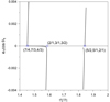Fig. A.1 Circular family for the unperturbed case at e1 = 0 and examples of families in the G4BP deflected from the resonant periodic orbits found by Eq. A.12 at $\left(\frac{T_2}{T_1},\frac{T_3}{T_1},\frac{T_3}{T_2}\right)=\left(\frac{5}{2},\frac{5}{1},\frac{2}{1}\right)$ for $k=3,\left(\frac{2}{1},\frac{3}{1},\frac{3}{2}\right)$ for k = $k=4,\left(\frac{7}{4},\frac{7}{3},\frac{4}{3}\right)$ for k = 5 (blue circles) computed for m1 = m2 = m3 = 10–6.

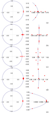Fig. A.2 Examples of distribution of eigenvalues (red dots) with respect to the complex unit circle with a magnification on the right of each panel for particular orbits from the families of the 1:2:3 resonant chain. (a) Triple instability with three pairs of real eigenvalues (S1 family); (b) Double instability with two pairs of real eigenvalues (S3 family); (c) u-complex instability with one pair of real and two pairs of complex eigenvalues outside the unit circle (S5 family); (d) Complex instability with two pairs of complex eigenvalues outside the unit circle, while the rest remain on it (S5 family). (e) Linear stability with all pairs on the unit circle (S1 family).

We note that the bifurcation points of the circular family can generate different families of the same resonant chain, which differ in the phases of planetary configurations. These configurations correspond to the initial location at t = 0 of the 3 bodies, namely p₁, p₂, and p₃, on the x-axis and are reflected on the values of the longitudes of pericenter and the mean anomalies of the periodic orbits in the G4BP.

Appendix B Orbital stability

B.1 Linear stability of periodic orbits

Let us denote with the vector x = (x₁,…,x₁₀) the set of ten variables of the system {x₁, x₂, x₃, y₂, y₃, x₁, x₂, x₃, y₂, y₃}. Then the solution x = x(t; x₀) corresponds to the initial conditions x0 = x(0). The variational equations of the system in Eq. A.6 and their solutions are written as: $$\begin{array}{lll}\dot{\eta }=J\left(t\right)\eta \hfill & \Rightarrow \hfill & \eta =\text{Δ}\left(t\right){\eta }_0,\hfill \end{array}$$(B.1)

where J is the Jacobian matrix of the system and A(t) is the fundamental matrix of solutions (called also matrizant or state transition matrix).

If the solution x(t; x₀) corresponds to a periodic orbit of period T, ∆(T) is the monodromy matrix. If and only if all the eigenvalues (shown with red dots in Fig A. 2) of ∆(T) lie on the complex unit circle, the periodic orbit is classified as linearly stable and η(t) remains bounded.

We remark that the eigenvalues are in conjugate pairs, as ∆(T) is symplectic. Moreover, due to the existence of the energy integral, one pair of eigenvalues (denoted here by λ₁ and λ₂) is always equal to unity. Some possible configurations of the other four pairs of eigenvalues and different types of instability are shown in Fig. A.2.

B.2 Chaotic Indicator

Establishing whether the eigenvalues lie on the unit circle or not can sometimes become an ambiguous process due to the limited accuracy. Therefore, apart from the linear stability along a family of periodic orbits, we also computed a chaotic indicator and, in particular, a simple detrended Fast Lyapunov Indicator (DFLI, e.g., Voyatzis 2008) defined as $$DFLI\left(t\right)=log\left(\frac{1}{t}\Vert \xi \left(t\right)\Vert \right),$$(B.2)

where ξ is the deviation vector computed after numerical integration of the variational equations. In Fig B. 1, we illustrate the DFLI’s behavior for the system Kepler-51. For a stable periodic orbit its evolution remains almost constant over time and takes small values, whereas it increases exponentially when the orbit is unstable.

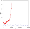Fig. B.1 Evolution of DFLI for an unstable (red) and a linearly stable (blue) periodic orbit with eigenvalues shown in panel (a) and (e) in Fig. A.2, respectively.

References

All Tables

All Figures

Fig. 1 Groups of families, Si (i = 1…6), of planar symmetric periodic orbits in the 1:2:3 resonant chain with stable segments close to the dynamical vicinity of Kepler-51 presented on the (e1, e2) and (e2, e3) planes. Each of these six groups consists of families of the same configuration (shown in Table 3), but with different planetary mass-ratios, that is, ${\rho }_i=\frac{m_c}{m_d}\text{and}{\rho }_o=\frac{m_c}{m_d}$ (shown in Table 1 and labeled from 1 to 4 on each panel). Label 1 corresponds to Masuda (2014), label 2 to Libby-Roberts et al. (2020), label 3 to default, and label 4 to high-mass priors considered by Battley et al. (2021). The stable (unstable) periodic orbits are depicted by blue (red) solid curves.

In the text

Fig. 2 Families, Si (i = 1…9), of planar symmetric periodic orbits in the 1:2:3 resonant chain close to the dynamical vicinity of Kepler-51 (top panels) and until their termination points (bottom panels) presented on the (e1 cos θ1, e2 cos θ2) and (e2 cos θ2, e3 cos θ3) planes. The angles for the different configurations of the families are shown in Table 3. Kepler-51 is identified in the top panels by the cyan “+” symbol, while the errors provided by Masuda (2014) are delineated by magenta dashed lines.

In the text

Fig. 3 DS-maps on the (e1, e2) and (e2, e3) planes, where the family S6 is projected, and the (∆ϖ21, ∆M21) and (∆ϖ32, ∆M32) planes. Kepler-51 is identified by the magenta “+” symbol, while the errors are delineated by magenta dashed lines. The color bar illustrates the DFLI values; dark colors correspond to regular evolution, while pale ones signify chaoticity. RL indicates that both pairs of planets are locked in a two-body MMR (2/1 and 3/2 MMR), while RS,L indicates the 1/1 secondary resonance inside the 2/1 MMR for the inner pair and a locking in the 3/2 MMR for the outer pair of planets.

In the text

Fig. 4 DS-maps on the eccentricity planes (e1, e2) and (e2, e3), where the family S5 is projected. RL denotes a two-body MMR (2/1 and 3/2 MMR for the inner and outer pairs of planets), RT indicates a three-body Laplace-like resonance (1:2:3 resonant chain), while RSA indicates the 1/1 secondary resonance inside the 2/1 MMR for the inner pair and an apsidal difference oscillation/rotation observed for the outer pair of planets. Colors and lines as in Fig. 3.

In the text

	Fig. 5 DS-maps on the eccentricity planes (e1, e2) and (e2, e3), where the family S1 is projected. Rs,a indicates the 1/1 secondary resonance inside the 2/1 MMR for the inner pair and an apsidal difference oscillation/rotation observed for the outer pair of planets. Colors and lines as in Fig. 3.
In the text

Fig. 6 DS-maps that showcase the extent of the 2/1 (left panels) and the 3/2 (right panels) distinct RL regions appear at the values$\frac{a_2}{a_1}\approx 1.58\text{and}\frac{a_3}{a_2}\approx 1.31$. The magenta lines showcase the nominal values of each MMR. The system Kepler-51 (magenta dashed lines enclosing the “+” symbol) is found at $\frac{a_c}{a_b}\approx 1.527\text{and}\frac{a_d}{a_c}\approx 1.325$, where an apsidal resonance takes place. Colors and lines as in Fig. 3.

In the text

	Fig. 7 Evolution of the orbital elements and resonant angles along an orbit initiated by the non-resonant low-eccentricity orbits, showcasing an apsidal resonance (shown in Fig. 6).
In the text

	Fig. 8 Evolution of the orbital elements and resonant angles along orbits initiated by the RL region (left panel) and the RS,L region (right panel) dynamically unveiled by the S6 family (shown in Fig. 3).
In the text

	Fig. 9 Evolution of the orbital elements and resonant angles along orbits initiated by the RL region (left panel) and the RT region (right panel) dynamically unveiled by the S5 family (shown in Fig. 4).
In the text

	Fig. 10 Evolution of the orbital elements and resonant angles along orbits initiated by the Rs,a regions dynamically unveiled by the S5 (left panel) and S1 (rightpanel) families (shown in Figs. 4 and 5, respectively).
In the text

Fig. A.1 Circular family for the unperturbed case at e1 = 0 and examples of families in the G4BP deflected from the resonant periodic orbits found by Eq. A.12 at $\left(\frac{T_2}{T_1},\frac{T_3}{T_1},\frac{T_3}{T_2}\right)=\left(\frac{5}{2},\frac{5}{1},\frac{2}{1}\right)$ for $k=3,\left(\frac{2}{1},\frac{3}{1},\frac{3}{2}\right)$ for k = $k=4,\left(\frac{7}{4},\frac{7}{3},\frac{4}{3}\right)$ for k = 5 (blue circles) computed for m1 = m2 = m3 = 10–6.

In the text

Fig. A.2 Examples of distribution of eigenvalues (red dots) with respect to the complex unit circle with a magnification on the right of each panel for particular orbits from the families of the 1:2:3 resonant chain. (a) Triple instability with three pairs of real eigenvalues (S1 family); (b) Double instability with two pairs of real eigenvalues (S3 family); (c) u-complex instability with one pair of real and two pairs of complex eigenvalues outside the unit circle (S5 family); (d) Complex instability with two pairs of complex eigenvalues outside the unit circle, while the rest remain on it (S5 family). (e) Linear stability with all pairs on the unit circle (S1 family).

In the text

	Fig. B.1 Evolution of DFLI for an unstable (red) and a linearly stable (blue) periodic orbit with eigenvalues shown in panel (a) and (e) in Fig. A.2, respectively.
In the text

References

- Antoniadou, K. I. 2016, Eur. Phys. J. Sp. Topics, 225, 1001 [NASA ADS] [CrossRef] [Google Scholar]
- Antoniadou, K. I., & Libert, A.-S. 2018, Celest. Mech. Dyn. Astron., 130, 41 [NASA ADS] [CrossRef] [Google Scholar]
- Antoniadou, K. I., & Voyatzis, G. 2013, Celest. Mech. Dyn. Astron., 115, 161 [Google Scholar]
- Antoniadou, K. I., & Voyatzis, G. 2014, Ap&SS, 349, 657 [NASA ADS] [CrossRef] [Google Scholar]
- Antoniadou, K. I., & Voyatzis, G. 2016, MNRAS, 461, 3822 [NASA ADS] [CrossRef] [Google Scholar]
- Battley, M. P., Kunimoto, M., Armstrong, D. J., & Pollacco, D. 2021, MNRAS, 503, 4092 [CrossRef] [Google Scholar]
- Berger, T. A., Huber, D., Gaidos, E., & van Saders, J. L. 2018, ApJ, 866, 99 [NASA ADS] [CrossRef] [Google Scholar]
- Charalambous, C., Martí, J. G., Beaugé, C., & Ramos, X. S. 2018, MNRAS, 477, 1414 [NASA ADS] [CrossRef] [Google Scholar]
- Christiansen, J. L., Crossfield, I. J. M., Barentsen, G., et al. 2018, AJ, 155, 57 [Google Scholar]
- Cochran, W. D., Fabrycky, D. C., Torres, G., et al. 2011, ApJS, 197, 7 [NASA ADS] [CrossRef] [Google Scholar]
- Fabrycky, D. C., Lissauer, J. J., Ragozzine, D., et al. 2014, ApJ, 790, 146 [Google Scholar]
- Freudenthal, J., von Essen, C., Ofir, A., et al. 2019, A&A, 628, A108 [NASA ADS] [CrossRef] [EDP Sciences] [Google Scholar]
- Gajdoš, P., Vaňko, M., & Parimucha, Š. 2019, Res. Astron. Astrophys., 19, 041 [Google Scholar]
- Gillon, M., Triaud, A. H. M. J., Demory, B.-O., et al. 2017, Nature, 542, 456 [NASA ADS] [CrossRef] [Google Scholar]
- Goździewski, K., & Migaszewski, C. 2020, ApJ, 902, L40 [CrossRef] [Google Scholar]
- Goździewski, K., Migaszewski, C., Panichi, F., & Szuszkiewicz, E. 2016, MNRAS, 455, L104 [Google Scholar]
- Hadden, S., & Lithwick, Y. 2014, ApJ, 787, 80 [Google Scholar]
- Hadden, S., & Lithwick, Y. 2017, AJ, 154, 5 [Google Scholar]
- Hadden, S., & Payne, M. J. 2020, AJ, 160, 106 [NASA ADS] [CrossRef] [Google Scholar]
- Hadjidemetriou, J. D. 1976, Ap&SS, 40, 201 [NASA ADS] [CrossRef] [Google Scholar]
- Hadjidemetriou, J. D. 1977, Celest. Mech., 16, 61 [NASA ADS] [CrossRef] [Google Scholar]
- Hadjidemetriou, J. D. 1980, Celest. Mech., 21, 63 [NASA ADS] [CrossRef] [Google Scholar]
- Hadjidemetriou, J. D., & Michalodimitrakis, M. 1981, A&A, 93, 204 [NASA ADS] [Google Scholar]
- Heller, R., Rodenbeck, K., & Hippke, M. 2019, A&A, 625, A31 [NASA ADS] [CrossRef] [EDP Sciences] [Google Scholar]
- Hénon, M. 1997, Lecture Notes in Physics Monographs, Generating Families in the Restricted Three-Body Problem (Berlin Heidelberg: Springer-Verlag), 52 [Google Scholar]
- Holczer, T., Mazeh, T., Nachmani, G., et al. 2016, ApJS, 225, 9 [Google Scholar]
- Leleu, A., Alibert, Y., Hara, N. C., et al. 2021, A&A, 649, A26 [NASA ADS] [CrossRef] [EDP Sciences] [Google Scholar]
- Lemaitre, A., & Henrard, J. 1990, Icarus, 83, 391 [NASA ADS] [CrossRef] [Google Scholar]
- Libby-Roberts, J. E., Berta-Thompson, Z. K., Désert, J.-M., et al. 2020, AJ, 159, 57 [Google Scholar]
- Lissauer, J. J., & Gavino, S. 2021, Icarus, 364, 114470 [NASA ADS] [CrossRef] [Google Scholar]
- Lissauer, J. J., Ragozzine, D., Fabrycky, D. C., et al. 2011, ApJS, 197, 8 [Google Scholar]
- Maffione, N. P., Darriba, L. A., Cincotta, P. M., & Giordano, C. M. 2011, Celest. Mech. Dyn. Astron., 111, 285 [Google Scholar]
- Masuda, K. 2014, ApJ, 783, 53 [Google Scholar]
- Michalodimitrakis, M., & Grigorelis, F. 1989, J. Astrophys. Astron., 10, 347 [NASA ADS] [CrossRef] [Google Scholar]
- Mills, S. M., Fabrycky, D. C., Migaszewski, C., et al. 2016, Nature, 533, 509 [Google Scholar]
- Morbidelli, A. 2002, Modern Celestial Mechanics: Aspects of Solar System Dynamics (Boca Raton, Florida, USA: CRC Press) [Google Scholar]
- Morrison, S. J., Dawson, R. I., & MacDonald, M. 2020, ApJ, 904, 157 [NASA ADS] [CrossRef] [Google Scholar]
- Morton, T. D., Bryson, S. T., Coughlin, J. L., et al. 2016, ApJ, 822, 86 [Google Scholar]
- Orosz, J. A., Welsh, W. F., Haghighipour, N., et al. 2019, AJ, 157, 174 [NASA ADS] [CrossRef] [Google Scholar]
- Panichi, F., Goździewski, K., Migaszewski, C., & Szuszkiewicz, E. 2018, MNRAS, 478, 2480 [NASA ADS] [CrossRef] [Google Scholar]
- Petit, A. C. 2021, Celest. Mech. Dyn. Astron., 133, 39 [NASA ADS] [CrossRef] [Google Scholar]
- Pichierri, G., & Morbidelli, A. 2020, MNRAS, 494, 4950 [Google Scholar]
- Siegel, J. C., & Fabrycky, D. 2021, AJ, 161, 290 [NASA ADS] [CrossRef] [Google Scholar]
- Steffen, J. H., Fabrycky, D. C., Agol, E., et al. 2013, MNRAS, 428, 1077 [NASA ADS] [CrossRef] [Google Scholar]
- Tamayo, D., Gilbertson, C., & Foreman-Mackey, D. 2021, MNRAS, 501, 4798 [NASA ADS] [CrossRef] [Google Scholar]
- Voyatzis, G. 2008, ApJ, 675, 802 [Google Scholar]
- Voyatzis, G. 2016, Eur. Phys. J. Sp. Topics, 225, 1071 [NASA ADS] [CrossRef] [Google Scholar]
- Weiss, L. M., Marcy, G. W., Petigura, E. A., et al. 2018, AJ, 155, 48 [Google Scholar]
As seen in exoplanet.eu in March 2022.
In Appendix A.1, we provide more details about the model set-up and the inertial and rotating frames of reference.
Asymmetric periodic orbits also exist, having longitudes of pericenter different than 0 or n, which are not considered herein.
Asymmetric configurations in resonant chains may also exist, but indications of such stability domains in three-planet systems were found in moderate eccentricity values when Jovian masses were assumed for the three planets (Voyatzis 2016).
(non-zero masses) describing nearly circular motion.
All Tables
Published data related to the planetary masses of Kepler-51 considered in this study.
Configurations of families of symmetric periodic orbits in the 1:2:3 resonant chain.