| Issue |
A&A
Volume 661, May 2022
|
|
|---|---|---|
| Article Number | A68 | |
| Number of page(s) | 12 | |
| Section | Stellar structure and evolution | |
| DOI | https://doi.org/10.1051/0004-6361/202142662 | |
| Published online | 03 May 2022 | |
Recurrent X-ray flares of the black hole candidate in the globular cluster RZ 2109 in NGC 4472
1
Scuola Universitaria Superiore IUSS Pavia, Palazzo del Broletto, Piazza della Vittoria 15, 27100 Pavia, Italy
e-mail: andrea.tiengo@iusspavia.it
2
Istituto Nazionale di Astrofisica, Istituto di Astrofisica Spaziale e Fisica Cosmica di Milano, Via A. Corti 12, 20133 Milano, Italy
3
Istituto Nazionale di Fisica Nucleare, Sezione di Pavia, Via A. Bassi 6, 27100 Pavia, Italy
4
Dipartimento di Fisica “Aldo Pontremoli”, Università degli Studi di Milano, Via G. Celoria 16, 20133 Milano, Italy
5
Laboratoire des 2 Infinis – Toulouse (L2IT-IN2P3), Université de Toulouse, CNRS, UPS, 31062 Toulouse Cedex 9, France
6
Astronomisches Rechen-Institut. Zentrum für Astronomie der Universität Heidelberg, Mönchhofstrasse 12-14, Heidelberg 69120, Germany
7
Istituto Nazionale di Astrofisica, Osservatorio Astronomico di Brera, Via E. Bianchi 46, 23807 Merate, Italy
8
Department of Physics, University of Milano-Bicocca, Piazza della Scienza 3, 20126 Milano, Italy
Received:
15
November
2021
Accepted:
15
February
2022
We report the systematic analysis of the X-ray observations of the ultraluminous X-ray source XMMU J122939.7+075333 located in the globular cluster RZ 2109 in the Virgo galaxy NGC 4472. The inclusion of observations and time intervals ignored in previous works and the careful selection of extraction regions and energy bands have allowed us to identify new flaring episodes, in addition to those that made it one of the best black hole candidates in globular clusters. Although most observations are too short and sparse to recognize a regular pattern, the spacing of the three most recent X-ray flares is compatible with a recurrence time of ∼34 h. If confirmed by future observations, this behavior together with the soft spectrum of the X-ray flares would be strikingly similar to the quasiperiodic eruptions recently discovered in galactic nuclei. Following one of the possible interpretations of these systems and of a peculiar class of extragalactic X-ray transients, we explore the possibility that XMMU J122939.7+075333 might be powered by the partial disruption of a white dwarf by an intermediate-mass (M ∼ 700 M⊙) black hole.
Key words: X-rays: individuals: XMMU J122939.7+075333 / galaxies: star clusters: individual: RZ 2109 / stars: black holes
© ESO 2022
Received 15 November 2021 / Accepted 15 February 2022
1. Introduction
XMMU J122939.7+075333 is an ultraluminous X-ray source (ULX) in the RZ 2109 globular cluster (GC) in the Virgo giant elliptical galaxy NGC 4472 (M49; Rhode & Zepf 2001) at a distance of 17.1 Mpc (Tully et al. 2008). Because its luminosity exceeds the Eddington limit for a neutron star and because of its variability (ruling out that its high luminosity might be due to the combination of multiple X-ray sources), XMMU J122939.7+075333 is one of the most robust black hole (BH) candidates in a GC (Maccarone et al. 2007). The census of BHs in GCs is an important route to test models of BH formation and of GC dynamical evolution (e.g., Morscher et al. 2015; Arca Sedda et al. 2018; Giesers et al. 2019).
XMMU J122939.7+075333 is peculiar also in the optical band: its spectrum shows a very bright and broad [O III] emission line, which implies a large overabundance of oxygen and high-speed outflows (Zepf et al. 2007). Moreover, this line appears to be emitted by a spatially resolved nebula (Peacock et al. 2012) and displays pronounced flux variability (Dage et al. 2019). The optical and X-ray peculiarities of XMMU J122939.7+075333 have been interpreted by invoking different scenarios: a stellar mass BH accreting close to its Eddington limit from a low-mass companion (Zepf et al. 2008), a nova shell illuminated by an external X-ray source (Ripamonti & Mapelli 2012), and the tidal disruption (or detonation; Irwin et al. 2010) of a white dwarf (WD; Clausen & Eracleous 2011) caused by an intermediate mass BH (IMBH).
The X-ray variability of XMMU J122939.7+075333 is a key piece of the puzzle to identify the nature of the compact object, the origin of the accreting matter, and the physical processes producing its powerful electromagnetic emission. Marked variability has been reported both within single observations (Maccarone et al. 2007; Stiele & Kong 2019) and by comparing the average flux of different observations (Joseph et al. 2015; Dage et al. 2018). In this paper, we report the discovery of more episodes of significant and possibly regular variability in archival XMM-Newton and Chandra observations of XMMU J122939.7+075333, including time periods affected by high particle background that were excluded in previous analyses. The peculiar variability pattern of XMMU J122939.7+075333 was identified within a broader search for flaring sources in the soft X-ray sky that was carried out via tools developed as part of the EXTraS project (De Luca et al. 2021) that were applied to all the XMM-Newton observations performed until the end of 2018. Through the analysis of a larger data set that also included archival Einstein and ROSAT observations and through a better characterization of high and low flux states, we were able to perform a more comprehensive and detailed study of the XMMU J122939.7+075333 X-ray spectra at different flux levels and of its long-term evolution.
2. X-ray observations and data analysis
2.1. XMM-Newton observations
XMMU J122939.7+075333 was observed eight times by XMM-Newton from 2002 to 2016. The observation log is reported in Table 1. All observations were processed using SAS 18.0.0 and the most recent calibration files. Since the exposures of the three EPIC cameras are not always perfectly simultaneous and the EPIC-pn (Strüder et al. 2001) is much more sensitive than the EPIC-MOS (Turner et al. 2001) in the soft energy band, where most of the variable X-ray emission of XMMU J122939.7+075333 is concentrated, the analysis of the XMM-Newton observations is based mainly on EPIC-pn data. The data of the two EPIC MOS cameras, when available, were checked for consistency.
X-ray observations of XMMU J122939.7+075333.
All the EPIC cameras were equipped with the thin filter and operated in full-frame mode. To subtract the background contribution properly, even during periods of high contamination by particle flares, we used a relatively small extraction region (a circle with a 15″ radius, containing ∼70% of the counts from a point source) for the source and a nearby region that was about ten times larger (on the same chip and free of apparent X-ray sources) to estimate and subtract the local background. According to standard procedures, only single- and double-pixel EPIC-pn events, with a PATTERN flag from 0 to 4, were selected.
2.2. Chandra observations
Chandra observed the position of XMMU J122939.7+075333 12 times between 2000 and 2019 with different CCDs of the ACIS (Garmire et al. 2003) S and I arrays (Table 1). The data were processed and reduced using the CIAO 4.11 software package and the calibration files in CALDB 4.8.2. The source data were selected from elliptical regions of sizes chosen so as to include ∼95% of the point-spread function (PSF; depending on the off-axis distance, their semimajor axes vary from ∼7.5 to 13.5 arcsec). The background was estimated from nearby regions. The spectra, the spectral redistribution matrices, and the ancillary response files were created using specextract. For the observations in which XMMU J122939.7+075333 was not detected, we set upper limits using the CIAO tool aprates.
2.3. ROSAT observations
The Roentgen Satellite (ROSAT; Pfeffermann et al. 1987) pointed at the NGC 4472 galaxy in December 1992 (a short 7 ks exposure with the HRI and then a deeper 25 ks with the PSPC) and in 1994, between June 19 and July 9 (27 ks with the HRI). The average off-axis angles and source net count rates are reported in Table 1. The HRI rates are taken from the ROSAT HRI Pointed Observations catalog (1RXH; ROSAT Scientific Team 2000), and the PSPC rate was computed by extracting the source counts from a circle with a 54″ radius and subtracting the background contribution from a nearby region. The same regions were also used to extract the source light curve, spectrum, and corresponding spectral matrix. The HRI light curves were instead extracted from 10″ circular regions.
2.4. Einstein observations
The Einstein observatory (Giacconi et al. 1979) observed the Virgo field including NGC 4472 multiple times between the end of 1979 and the beginning of 1981. In particular, the Einstein High Resolution Imager (HRI) instrument observed XMMU J122939.7+075333 at an off-axis angle of ∼7′ for a cumulative net exposure time of ∼33 ks (Table 1). The analysis reported here is based on the image and automatic source detection produced by the Einstein HRI Catalog of ESTEC Sources (HRIEXO)1. The image distinctly displays a point source at the position of XMMU J122939.7+075333 and the catalog reports a source with ∼80 net counts at a distance < 6″ from its coordinates.
3. Results
3.1. Short-term X-ray variability
The light curves of XMMU J122939.7+075333 in four energy bands registered by the EPIC-pn during three consecutive XMM-Newton orbits in January 2016 are shown in Fig. 1. Three flares are clearly detected, mainly in the soft energy bands (E < 1 keV). The first two flares were already discovered and discussed by Stiele & Kong (2019), whereas the flare that occurred during the last observation was missed because time intervals with high particle background were rejected. As shown mainly in the bottom panel of Fig. 1, a background flare occurs at the approximate time of the source flare, but its intensity in the softest energy bands (upper panels of Fig. 1) is much lower than the flux increase in the point source.
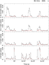 |
Fig. 1. EPIC-pn light curves (from top to bottom: 0.15–0.5 keV, 0.5–1 keV, 1–2 keV, and 2–8 keV) extracted from the source (black) and background (red) regions during the three XMM-Newton observations performed in 2016 (0761630101, 0761630201, and 0761630301). The background count rates (and error bars) are rescaled by a factor 10 to account for the different sizes of the source and background regions. |
Although the profile of the three peaks significantly deviates from a Gaussian, we estimated their time separations and widths with a simple model consisting of a constant plus three Gaussian curves. When this model is applied to the 0.15–2 keV background-subtracted EPIC-pn light curve ( for 107 degrees of freedom, d.o.f.), the distances between the centroids of the first two Gaussian peaks and between the last two are 229 ± 0.5 and 111.9 ± 0.7 ks, respectively. The FWHM of the three Gaussian peaks are 26.6 ± 0.9, 14.1 ± 0.7, and 16.7 ± 1.4 ks.
We also checked the energy dependence of these parameters by fitting the background-subtracted EPIC-pn light curves also in the 0.15–0.5, 0.5–1, and 1–2 keV energy bands with the same model. Although the left panel of Fig. 2 shows a slight decrease in peak separation with energy, this trend is not statistically significant. The FWHM (right panel of Fig. 2) displays a significant increase with energy for the first peak, but no statistically significant trend can be derived for the second and third peaks.
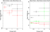 |
Fig. 2. Energy dependence of the peak separation (left panel) and FWHM (right panel) of the three flares observed in the 2016 XMM-Newton observations in three energy bands and in the 0.15–2 keV total range. The separation between the first two flares has been divided by 2 in order to compare it with the separation between the last two flares. |
It is interesting to note that the separation between the first two flares approximately doubles the distance between the last two peaks and that in case of a fixed recurrence time, one flare might have been missed because it occurred in the middle of the > 60 ks gap between the first two observations. A possible indication of such a flare might be present in the EPIC-pn light curve in the softest energy band (top panel of Fig. 1), where a small count-rate excess emerges at the beginning of the second exposure. A fit of the first 60 ks of the background-subtracted light curve with a constant function provides  for 19 d.o.f., corresponding to a null-hypothesis probability of 5 × 10⁻⁴. A similar excess is also present in the MOS light curve in the 0.15–1 keV energy band, but with a lower statistical significance (4 × 10⁻³), as expected because the effective area of the MOS cameras at very low energy is far smaller, which is only partly compensated for by the slightly earlier start of the MOS exposures.
The only other archival observations of XMMU J122939.7+075333 that allow us to test the hypothesis of a possible flare recurrence on timescales > 1 day are the two long observations performed by Chandra in 2011 at a distance of one week (Table 1). The ACIS-S light curves in three energy bands2 are shown in Fig. 3: significant variability is clearly detected in both observations3, against a fairly stable background.
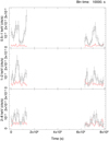 |
Fig. 3. ACIS-S light curves (from top to bottom: 0.5–1 keV, 1–2 keV, and 2–8 keV) extracted from the source (black) and background (red) regions during the two Chandra observations performed in 2011 (12888 and 12889). The background count rates (and error bars) are rescaled by a factor of 3 to account for the different sizes of the source and background regions. |
When the 0.5–2 keV background-subtracted light curve of each observation is fit with a constant plus two Gaussian curves ( for 7 d.o.f. and
  for 10 d.o.f., respectively), the distance between the two peaks in the first and second observation are 78.8 ± 5.3 and 68.4 ± 3.6 ks, respectively. The first and the last peaks, whose positions are rather well defined, occur at a distance of 668.7 ± 3.6 ks. We note that this distance would correspond to nine cycles of a 73.4 ks periodicity, which would be compatible with the separations of the peaks detected in the single observations. On the other hand, only these peaks are clearly observed in multiple energy bands and are fully included in the observations, and when we also consider the structured light-curve profile, we therefore cannot exclude a longer recurrence time. In particular, the separation between them would be compatible with six cycles of a ∼112 ks period, consistent with the recurrence time suggested by the 2016 observations.
The FWHMs of the four peaks are 24.3 ± 4.9, 25.2 ± 9.4, 12 ± 7.1, and 51.1 ± 10.4 ks. They are consistent with the range of peak widths measured in the EPIC-pn light curves (right panel of Fig. 2).
In addition to the prominent variability of XMMU J122939.7+075333 during these long observations and in the 2004 XMM-Newton observation already reported by Maccarone et al. (2007), we detected significant changes in the source count rate also in the 2008 XMM-Newton observation and in two out of the four observations performed in 2014 (Table 1). In January 2014, XMMU J122939.7+075333 was observed twice by XMM-Newton at such a large off-axis angle that it could be detected only by the EPIC-pn because it was outside the EPIC-MOS field of view. No source variability was detected in the first observation (0722670301), but during the second exposure (0722670601), we detected a significant count-rate increase without any corresponding background variation (Fig. 4). If we fit the 0.15–2 keV background-subtracted EPIC-pn light curve with a constant function, we obtain an unacceptable  of 8.8 for 4 d.o.f.
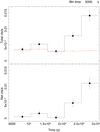 |
Fig. 4. EPIC-pn light curves in the 0.15–2 keV energy band during observation 0722670601. Top panel: light curve extracted from the source (black squares) and background (red) regions. The background count rates (and error bars) are rescaled by a factor 12 to account for the different sizes of the source and background regions. Bottom panel: background-subtracted light curve. |
Chandra observed XMMU J122939.7+075333 three times between April 2014 and February 2015, but detected it significantly only on one occasion (observation 16260). The corresponding light curve in the 0.3–2 keV energy band is shown in Fig. 5 and appears to be variable. By fitting the background-subtracted light curve with a constant count rate, we obtain a  for 5 d.o.f., corresponding to a null-hypothesis probability of 2 × 10⁻³.
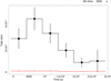 |
Fig. 5. ACIS-S light curve in the 0.3–2 keV energy band extracted from the source (black squares) and background (red) regions during observation 16260. The background count rates (and error bars) are rescaled by a factor 25 to account for the different sizes of the source and background regions. |
Finally, during a very short observation performed in 2008 that was affected by strongly variable background, the EPIC-pn detected a sharp decrease in the net count rate of XMMU J122939.7+075333 (Fig. 6). Since the statistical significance of the deviation from a constant rate is rather low ( for 3 d.o.f., corresponding to a null-hypothesis probability of 10−2), we also examined the light curve accumulated by the EPIC MOS1 and MOS2 detectors, which started observing earlier. The background-subtracted light curve obtained by combining the data of the two EPIC-MOS cameras is perfectly consistent with a constant count rate (
 for 5 d.o.f.; bottom panel of Fig. 6). However, we note that the EPIC-MOS observed XMMU J122939.7+075333 mostly before the flux drop indicated by the EPIC-pn light curve, and it detected an average count rate of (1.8 ± 0.3) × 10−2 cts s−1, which is far higher than the rate observed during quiescent periods. For example, during the second 2016 observation (0761630201), the average EPIC-MOS count rate was (0.39 ± 0.03) × 10−2 cts s−1. If we separate the quiescent and flare time intervals by applying a count-rate threshold of 0.01 cts s−1 to the 0.15–1 keV EPIC-pn light curve, the count rates during quiescence and the flare were (0.14 ± 0.03) × 10−2 cts s−1 and (1.25 ± 0.08) × 10−2 cts s−1, respectively. Despite the much lower efficiency of the EPIC-MOS at low energies and the earlier stop of the 2008 MOS exposures, these data support the marginal detection of a flare in the 2008 EPIC-pn data.
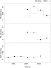 |
Fig. 6. Light curves in the 0.15–2 keV energy band during the 2008 XMM-Newton observation (0510011501). Top panel: EPIC-pn light curve extracted from the source (black squares) and background (red) regions. The background count rates (and error bars) are rescaled by a factor of 10 to account for the different sizes of the source and background regions. Middle panel: EPIC-pn background-subtracted light curve. Bottom panel: EPIC MOS1+MOS2 background-subtracted light curve. |
The light curves extracted from the ROSAT data do not display any significant variability. However, since the satellite was in low Earth orbit, these light curves are not continuous, and they are less sensitive to variability on timescales of a few hours.
3.2. Spectral analysis of the 2016 XMM-Newton observations
The clear identification of three flares in the 2016 XMM-Newton observations means that the X-ray spectra of XMMU J122939.7+075333 at different flux levels can be compared better than in previous works (e.g., Maccarone et al. 2007; Joseph et al. 2015; Stiele & Kong 2019). Specifically, we analyzed the EPIC-pn spectra of the quiescent and flare states during each of the three observations and adopted the same count-rate threshold as in Sect. 3.1. The spectral analysis was performed using XSPEC v12.10.1. The absorption component was fixed at the foreground Galactic value (NH = 1.55 × 1020 cm−2, assuming solar abundances from Wilms et al. 2000). A distance of 17.1 Mpc (Tully et al. 2008) was assumed to compute the source luminosity (and derived quantities).
From a simultaneous fit of the six EPIC-pn spectra with a TBabs*(pegpwrlw + diskbb + gaussian) model, with the Gaussian line intrinsic width and centroid fixed at 0 and 0.65 keV, respectively, we obtained the parameters reported in Table 2. The spectra and residuals with respect to the model are shown in Fig. 7. As already noted in previous works, the spectrum during the flare is much softer. In this spectral deconvolution, the spectral softening can be attributed to the appearance of a disk component only during the flare and a corresponding increase by about an order of magnitude of the flux of the emission line, which, as already proposed by Joseph et al. (2015), can readily be identified as O VIII. At the same time, the hard power-law component characterizing the bulk of quiescent emission significantly also increases during flares, but only by a factor of ∼2. Except for the normalization of the disk component of the last flare, which shows a lower peak flux in the soft energy band (Fig. 1), the parameters of the two spectral states are consistent in the three observations.
Best-fit parameters of the EPIC-pn spectra during flares and quiescence in the 2016 XMM-Newton observations.
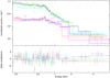 |
Fig. 7. EPIC-pn spectra (upper panel) and residuals with respect to the best-fit model with parameters in Table 2 (lower panel) of XMMU J122939.7+075333 in observations 0761630101 (black during flare, red in quiescence), 0761630201 (green during flare, blue in quiescence) and 0761630301 (cyan during flare, purple in quiescence). |
Since in previous works (e.g., Maccarone et al. 2007; Joseph et al. 2015) it was proposed that the low flux states of XMMU J122939.7+075333 might be caused by an excess of absorption, we tried to fit the six spectra keeping linked all the spectral parameters and adding a free additional absorption component, but the resulting fit was unacceptable ( for 276 d.o.f.; null hypothesis probability = 2.4 × 10⁻⁵). A much better fit (
 for 271 d.o.f.; null hypothesis probability = 6.5 × 10⁻²) is instead obtained by adding an overall free normalization factor to the model of each spectrum. In this case, the three flare spectra are consistent with no additional absorption and the quiescent spectra with an excess absorption of NH∼1021 cm−2. The overall normalization factors indicate that the flux of the third flare was ∼30% lower than that of the previous flares and that during the quiescent states, in addition to the excess absorption, the intrinsic source flux decreased by a factor ∼4.
3.3. Long-term X-ray variability
We applied the best-fit spectral model used for the 2016 observations with the normalizations of the three spectral components as free parameters to all the available PSPC, EPIC-pn and ACIS-S spectra with sufficient count statistics. When possible, we separated the flare and quiescent time periods4. This simple model provides acceptable fits to all the spectra, with the parameters displayed in Fig. 8. Their evolution does not show a clear long-term trend, but it illustrates the striking spectral difference between the quiescent and flaring states of XMMU J122939.7+075333 well. In the 2011 Chandra observation, where the flare and quiescent states cannot be clearly defined, the spectral parameters are somewhat intermediate between those of the two flux levels. The spectral parameters of all the remaining observations are instead compatible with those of the flare states.
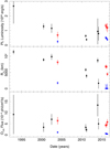 |
Fig. 8. Time evolution of the power-law 0.3–10 keV unabsorbed luminosity (upper panel), apparent inner disk radius (middle panel; from the diskbb model in XSPEC, assuming a disk inclination of 45°) and Gaussian line flux (lower panel) obtained by fitting the available spectra with the same model as in Table 2. Spectra extracted from the full observation, flare, and quiescent time intervals are represented by black circles, red stars and blue squares, respectively. The time separations between the exposures performed during the same year have been enhanced for clarity. |
Based on the best-fit parameters of the average spectrum of each observation (including those with poorly constrained parameters, not reported in Fig. 8), we derived the conversion factors from the 0.5–2 keV background subtracted count rate to the observed flux in the same energy range. From these conversion factors we converted the 0.5–2 keV light-curves of each XMM-Newton and Chandra observation, extracted from the same regions as the corresponding spectra, into luminosity units, obtaining Fig. 9. For the Chandra observations where XMMU J122939.7+075333 was not significantly detected, the upper limits on the source count-rates (Table 1) were converted into 3σ luminosity upper limits by assuming the spectral best-fit parameters of the first flare detected by XMM-Newton in 2016 (Table 2) and the ancillary response file associated to the regions from which the counts were extracted. If we instead adopted the spectral parameters of the quiescent state, depending on the detector efficiency at the lowest energies, the upper limits on luminosity would either remain virtually unchanged (e.g., in observation 11274) or be reduced by up to ∼40% (in observation 15760).
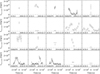 |
Fig. 9. Light curves and 3σ upper limits of XMMU J122939.7+075333 in luminosity units for all the XMM-Newton and Chandra observations in Table 1. The conversion from 0.5–2 keV count rates into luminosity in the 0.5–2 keV energy band was based on the best-fit parameters of the average spectrum for each observation. The upper limits were derived from the 0.3–2 keV count-rate limits in Table 1 assuming the best-fit spectral parameters of the first flare detected in 2016 (Table 2). Although Dage et al. (2019) report a 3σ detection in the 2019 observation, we set an upper limit because most of the counts were detected above 2 keV. The horizontal bars indicate either the bin size of the light curve (ranging from 1 to 10 ks) or the observation exposure time (for upper limits and observations with a single time bin). The start dates of the observations and the instrument are indicated in each panel. |
As already noted, the Einstein and ROSAT exposures were too fragmented to display meaningful light curves, and therefore, we only computed the average luminosity for these observations. For the ROSAT PSPC observation, we adopted the best-fit spectral parameters shown in Fig. 8 and obtained a 0.5–2 keV luminosity of (3.0 ± 0.3) × 1039 erg s−1. This is the highest flux level ever reached by XMMU J122939.7+075333 (see Fig. 9).
To convert the count rates detected during the Einstein and ROSAT HRI observations into luminosity, we used the WebPIMMS5 tool, assuming a simplified spectral model: a power law with photon index 3.7 and absorption NH = 1.55 × 1020 cm−2, which in the 0.5–2 keV energy range satisfactorily fits the spectrum of the first flare detected by XMM-Newton in 2016 ( for 25 d.o.f.). The source count rates reported in Table 1 correspond to (8.6 ± 1.4) × 1038 erg s−1 for the Einstein HRI observation and (1.1 ± 0.2) × 1039 erg s−1 and (1.1 ± 0.1) × 1039 erg s−1 for the ROSAT HRI observations performed in 1992 and 1994, respectively. The analysis of the latter exposure was reported also by Maccarone et al. (2010), who used a different spectral model, source distance, and energy range to estimate the luminosity, however. In the same work, they reported a nondetection with Einstein in 1978, but they did not mention the detection in the HRIEXO catalog reported here. They also reported the analysis of Swift Neil Gehrels Observatory/XRT observations taken in 2007, 2008, and 2010, which indicate that XMMU J122939.7+075333 was not persistently in the bright state. These exposures are too short and sparse, however, to constrain the possible presence of flares with a duration of a few hours.
4. Discussion
The systematic and detailed analysis of all available XMM-Newton and Chandra observations of XMMU J122939.7+075333, also including time periods with high and variable background, has allowed us to identify new episodes of source variability. In particular, since most of the variability is concentrated in the soft energy band, where the particle background contribution is less dramatic (see, e.g., Fig. 1), we paid special attention to the choice of the most convenient energy bands for the timing analysis. The detection of these additional X-ray flaring episodes is particularly important because they suggest a possible regular pattern (a periodicity or quasi-periodicity) and allow us to interpret the different spectral components and their evolution in the last decades more clearly.
4.1. Implications of time variability
The analysis of the long-term variability of XMMU J122939.7+075333 reported in previous works (e.g., Maccarone et al. 2010; Dage et al. 2018) was mostly based on the average fluxes and spectral parameters measured during each observation, without properly distinguishing flare and quiescent states. As a consequence, the extreme flux variability resulting from the comparison of observations with the source in different states was interpreted as a long-term trend and was used as an argument against the tidal disruption scenarios (Maccarone et al. 2010).
Figure 9 instead shows that the long-term evolution of the source luminosity in the 0.5–2 keV energy band is apparently characterized by fast transitions between bright and faint states, with rather stable intensity levels of ∼1–2 × 1039erg s−1 and ∼2 × 1038erg s−1, respectively. Defining as bright states all the time bins during which XMMU J122939.7+075333 was detected by XMM-Newton or Chandra above 5 × 1038 erg s−1, the source has been observed in the bright state for 37% of the ∼1.1 Ms total exposure time.
XMMU J122939.7+075333 was always in a bright state during the first Chandra and XMM-Newton observations, performed between 2000 and 2002, as well as during all the Einstein and ROSAT exposures taken from 1979 to 1994. Instead, XMMU J122939.7+075333 was below our luminosity threshold in the two most recent Chandra observations. Moreover, the fraction of time spent in the bright state was 42% between 2004 and 2015 and only 24% during the three long XMM-Newton observations performed in 2016. This suggests that before 2004, XMMU J122939.7+075333 might have been persistently or for a larger fraction of time in the bright state. However, the available data are too sparse and inhomogeneous, with observations characterized by different exposure duration and instrumental sensitivity, to robustly constrain a possible progressive reduction of the bright-state duty cycle.
As already noted in Sect. 3.1, the 2016 XMM-Newton data are compatible with a regular flaring activity with a periodicity of ∼110 ks, although both the flare duration, which is a factor ∼2 longer for the first peak, and the peak flux, which is ∼30% lower for the last flare, display some variability. The same variability pattern is also compatible with the 2004 XMM-Newton observation, which starts with the source at a high flux level and has a total duration of only 90 ks, however. Therefore, in this case, we can only set a lower limit of ∼30 ks on the high-flux state duration, which is consistent with the duration of the bright state in the first 2016 observation, and of ∼90 ks on the possible flare recurrence time.
Significant variability within the same luminosity limits was visible also during the two long observations performed by Chandra in 2011. If we interpret the count-rate excess detected at the end of the first observation and at the beginning of the second observation as part of a flare with a duration comparable to that of the other XMMU J122939.7+075333 X-ray flares, we derive a recurrence time of ∼70 ks. If we instead consider only the two flares that were fully contained in each exposure, their separation greater than one week, and the relatively long duration make them compatible with many possible recurrence times, including the ∼110 ks suggested by the 2016 XMM-Newton observations (Sect. 3.1).
The other currently available observations are too short to constrain the flare duration and recurrence time. The only exception might be XMM-Newton observation 0722670301 (9–10 January 2014), during which the source remained in the bright state for longer than in the longest flare detected in any other observation. However, this observation was affected by a high level of particle background, and the telemetry buffer of the EPIC-pn quadrant hosting XMMU J122939.7+075333 was saturated throughout the full observation. As a result, the lifetime of this exposure is only ∼30% of the total observation duration, and considering also that there are no simultaneous EPIC-MOS data, the sensitivity of this observation is lower than that of the other XMM-Newton observations.
On the other hand, as described in Sect. 3.1 and shown in Fig. 9, some short observations displayed rapid flux changes that are perfectly consistent with the variability pattern described above. Moreover, we note that after 2010, XMMU J122939.7+075333 has been detected about eight times in the high-flux state during ∼820 ks of XMM-Newton and Chandra observations, which is compatible with the ∼110 ks recurrence time of the flares suggested by the most recent data. Only long, possibly uninterrupted, observations with instruments with a large effective area at energies well below 1 keV, such as the EPIC-pn, and in the future, the X-IFU and WFI on board ATHENA (Nandra et al. 2013), will be able to establish firmly whether the flares of XMMU J122939.7+075333 occur randomly or are spaced regularly.
4.2. Implications of spectral analysis
The analysis of all the XMMU J122939.7+075333 X-ray spectra with sufficient data quality confirms that the spectra of the short observations with high flux are compatible with those observed during the flares that were detected during the four longest XMM-Newton observations (Fig. 8). In particular, the normalization of the disk component, which vanishes during the quiescent time periods, corresponds to an apparent inner disk radius ranging from ∼5000 to ∼10 000 km for an inclination of 45° . Applying Eq. (2) of Zampieri & Roberts (2009), with f = 1.7 and b = 15.6 , these values correspond to a BH mass between ∼600 and ∼1200 M⊙.
Assuming that the inner disk radius Rin represents a proxy for the BH ISCO, the BH mass is related to its spin according to
![$$ \begin{aligned} R_{\rm ISCO} = \frac{GM_{\rm BH}}{c^2}\left[ 3 + Z_2 - \mathrm{sign}(\xi )(3-Z_1)(3+Z_1+2Z_2) \right]^{1/2}, \end{aligned} $$](/articles/aa/full_html/2022/05/aa42662-21/aa42662-21-eq16.gif)
where Z1, 2 are functions of the BH dimensionless spin parameter ξ = SBH/MBH (Bardeen et al. 1972). The assumption of RISCO ≡ Rin = 6400 km (Table 2) and variation of SBH = 0–1 leads to a range of IMBH masses of MBH ≃ 700–4340 M⊙.
We note that the spin of the IMBH is intrinsically connected with its past evolution; it is most likely inherited from the IMBH formation history. As recently discovered in a number of numerical simulations of young massive clusters, IMBHs in the mass range 100–500 M⊙ can form either from the collision and merger of massive main-sequence stars (e.g., Di Carlo et al. 2021) or through the accretion of a massive star onto a stellar BH (e.g., Rizzuto et al. 2021). In this scenario, the spin of the nascent IMBH is probably either inherited from the collapse of the stellar merger remnant or from the stellar BH progenitor (see, e.g., Qin et al. 2019). In either case, the IMBH spin would not deviate much from the typical values expected for stellar BHs. There is currently little consensus about the BH natal spin distribution because it strongly depends on which stellar evolution recipes are adopted to model the BH formation.
On the other hand, IMBH seeds could also grow through repeated mergers of stellar BHs, provided that the host cluster is sufficiently massive and dense. This process tends to decrease the IMBH spin, depending on the number of merging events that contributed to its buildup (Arca Sedda et al. 2021a).
A further possibility is that the IMBH growth is regulated by the two processes above: first, an IMBH seed with a mass > 100 M⊙ forms via stellar collisions or accretion onto stellar BHs, and later, the IMBH grows further via repeated BH mergers (e.g., Arca-Sedda et al. 2021b; Rizzuto et al. 2021). Assuming that a population of IMBH seeds with masses in the range 100–500 M⊙ formed in globular clusters at redshift z = 2–6 (Katz & Ricotti 2013), Arca Sedda et al. (2021a) have recently shown that the overall population of IMBHs at redshift z < 1 would be characterized by a mass distribution that extends between 250–1500 M⊙, with a clear peak at around MBH ∼ 750 M⊙. Therefore, the possibility of measuring either the IMBH mass or its spin with high precision would provide us with crucial insights into the IMBH formation and evolution processes.
Another possible indication that XMMU J122939.7+075333 might host an IMBH is the high bolometric luminosity of this disk component, which ranges from 2 to 8 × 1039 erg s−1. The latter value is above the Eddington limit of a ∼10 M⊙ BH, but corresponds to < 10% of the Eddington luminosity of a 1000 M⊙ BH. However, this argument is not sufficient to prove the presence of an IMBH in the RZ 2109 GC, as demonstrated by the discovery of pulsations in ULXs (e.g., Bachetti et al. 2014; Israel et al. 2017), which implies that they can be powered even by neutron stars.
The comparison of the spectra of the bright and faint states of XMMU J122939.7+075333 also unveils a remarkable increase in O VIII emission line flux during the flares. This variability on a timescale of hours without delay with respect to the disk component appearance constrains the size of the emission region and its maximum distance from the accretion disk within 1015 cm. The intensity of the optical [O III] broad line is also variable from observation to observation (Dage et al. 2019), but HST spatially resolved spectra imply an emission region that is larger than a few parsecs (Peacock et al. 2012). Simultaneous X-ray and optical spectroscopic observations would be crucial to confirm whether a fraction of the [O III] flux might also be produced in a much more compact region.
The significantly higher flux of the power-law component in the bright state implies that the hard X-ray emission of XMMU J122939.7+075333 cannot be fully attributed to the cumulative X-ray emission of different objects in the RZ 2109 GC either. Specifically, the same compact source that causes the flares must be able to increase the 0.3–10 keV luminosity of its power-law spectral component by at least 5 × 1038 erg s−1 above a similarly bright quiescent luminosity, to which other unrelated X-ray sources might contribute. A hard component with this luminosity can be easily produced by a stellar and by an intermediate-mass accreting BH.
The possibility that a variable column density might fully account for the X-ray variability of XMMU J122939.7+075333 is ruled out by the simultaneous spectral fit of the 2016 XMM-Newton spectra at different intensity levels (Sect. 3.2). However, we showed that a combination of enhanced absorption and substantial flux reduction, possibly produced by the partial screening of the source emission by an optically thick structure, is consistent with the time-resolved spectral analysis of the same observations. Moreover, the morphology of the 2016 light curve suggests the interpretation of the high flux states of XMMU J122939.7+075333 as soft X-ray flares rather than short periods during which the X-ray emission leaks through a dense surrounding medium.
4.3. Comparison with other systems
The discovery of many episodes of bright and soft X-ray flares in the ULX XMMU J122939.7+075333, which might be regularly spaced in time, can be a crucial clue to interpreting this unique object. A quasi-periodic flaring behavior has recently been detected in another ULX in the galaxy NGC 3621; in this case, the timescale is only ∼1 hr and the X-ray spectrum is much harder (Motta et al. 2020). The brightest ULX known to date, HLX-1 in the ESO 243-49 galaxy, has shown a flaring variability mainly in the soft X-ray band with a periodicity of ∼1 yr, but this rather regular pattern has recently changed and possibly disappeared (Lin et al. 2020).
Moreover, the variability of XMMU J122939.7+075333 is strikingly similar to the quasi-periodic X-ray eruptions that repeat on timescales of several hours displayed by the active galactic nuclei (AGN) GSN 069 (Miniutti et al. 2019) and RX J1301.9+2747 (Giustini et al. 2020), as well as by two nuclear X-ray sources in previously quiescent galaxies (Arcodia et al. 2021) and in a tidal disruption event (TDE; Chakraborty et al. 2021). Their origin might be related to disk instabilities (e.g., Sniegowska et al. 2020), the partial disruption of an orbiting star (King 2020; Sheng et al. 2021), the self-lensing of a supermassive BH binary system (Ingram et al. 2021), or transient accretion in inspirals with an extreme mass ratio (Metzger et al. 2022; Zhao et al. 2021). Although their luminosity is much higher, we note that these flaring X-ray sources are also characterized by a very soft spectrum. Moreover, the regular variability of GSN 069 started after several years of bright persistent emission, as might have happened in the case of XMMU J122939.7+075333.
A Galactic X-ray source with interesting similarities with XMMU J122939.7+075333 is the BH candidate X9 at the center of the GC 47 Tuc (Miller-Jones et al. 2015): it displays flaring X-ray variability on an apparently regular timescale of ∼1 week and its X-ray spectrum is characterized by oxygen emission lines (Bahramian et al. 2017). Its luminosity, however, ranges from 1033 to 1034erg s−1, which is more than 5 orders of magnitude below that of XMMU J122939.7+075333, which in turn is more than 3 orders of magnitude less luminous than the QPEs observed in the galactic nuclei (Miniutti et al. 2019; Giustini et al. 2020; Arcodia et al. 2021; Chakraborty et al. 2021).
A particularly intriguing possibility is that these accreting sources, all located in extremely crowded regions (at the very centers of GCs or galaxies), might share a common mechanism that causes the modulation of their X-ray luminosity on different timescales, perhaps the interaction with a star, very likely on a highly eccentric orbit, that might perturb a preexisting disk or provide matter through partial tidal disruption. In addition, the partial tidal disruption of a star orbiting at a short distance from the supermassive BH at the center of our Galaxy has been proposed as the possible cause of the X-ray and near-IR flaring activity of Sgr A* (Leibowitz 2020).
Finally, Maccarone (2005) has proposed to interpret a small class of X-ray transients in the NGC 4697 galaxy (Sivakoff et al. 2005) as periodic accretion episodes of eccentric binary systems in GCs. More recently, after the discovery of other extragalactic X-ray transients with similar properties (Jonker et al. 2013; Irwin et al. 2016), Shen (2019) has interpreted these transients as partial tidal disruptions of WDs in eccentric (or parabolic) orbits around IMBHs. In the next section, we explore a similar scenario also for XMMU J122939.7+075333. Although the spectra of these transients are harder, their luminosities are higher, and their light curves have asymmetric profiles, we note that TDEs also display a rather rich X-ray phenomenology, including both soft and hard spectra (see Saxton et al. 2020 for a review). Because its variability timescale and luminosity are intermediate compared with all the phenomena reported above, XMMU J122939.7+075333 might be a crucial object based on which this unifying scenario might be clarified.
4.4. Partial tidal disruption scenario
We explored the possibility that the recurrent X-ray flares from XMMU J122939.7+075333 might be produced by an extreme mass transfer system in which the orbit of the secondary star is highly eccentric, so that the star fills its Roche lobe only at pericenter, losing a small amount of mass at each passage. Due to the implied high eccentricity (see below), we used the formalism developed for partial tidal disruption events (pTDE), where a star on a parabolic orbit is disrupted by a massive BH (see, e.g., Rees 1988; Guillochon & Ramirez-Ruiz 2013).
We define the stellar mass M* = m*M⊙ and radius R* = r*R⊙, and the BH mass MBH. The Roche lobe is given by Eggleton (1983)
where a is the semi-major axis, e is the orbital eccentricity, and the pericenter is rp = a(1 − e). The strength of this type of encounters is usually quantified through a dimensionless parameter called penetration factor, defined as6

where rt ≃ (MBH/M*)1/3R* is the maximum distance at which the star is fully disrupted by the BH (also known as the tidal radius). Generally speaking, if β ≲ 1 just a fraction of the stellar mass is stripped away and accreted onto the BH, and thus we have a pTDE. In terms of the Roche lobe, this means that at the pericenter,

hence if β ≲ 1, the lobe is just partially filled by the stellar material. Guillochon & Ramirez-Ruiz (2013) showed that when β drops below ∼0.5, the mass transfer virtually stops.
We estimate the value of β from the total mass accreted during each flare using the correlation obtained from hydrodynamical simulations of pTDE (Guillochon & Ramirez-Ruiz 2013). The total energy emitted by this source during each of the three 2016 XMM observations is

respectively. Assuming an accretion efficiency η = 0.1, we obtain that the total mass accreted onto the BH during each flare in units of solar masses is about

The observed large abundance of oxygen suggests that the star involved in the event is a WD. Considering a WD with a mass in the range 0.1 M⊙ ≤ M* ≤ 1.4 M⊙, we have that the ratio of the accreted mass over the stellar mass is in the following interval:
These low values of the ratio imply that the BH-WD encounters must be highly grazing and in a way that the β parameter needs to be very close to ∼0.5, with a weak dependence on the stellar structure, modeled as a polytropic sphere with index γ (Guillochon & Ramirez-Ruiz 2013; Eqs. A3–A9–A10). In particular, we obtain β ∼ 0.45 for γ = 4/3 and β ∼ 0.5 for γ = 5/3.
Because the accreted mass drops steeply when β becomes smaller than ≃0.5, the resulting β is very insensitive to the actual value of accreted mass. In other words, because ΔM/M* is very small, β has to be very close to ≃0.45 (or 0.5, depending on γ), with differences occurring only at the 0.1% level.
To also estimate the other orbital parameters of the event, we can proceed in the following way. From the best fit of the inner disk radius Rin ∼ 6400 km (Table 2) and Eq. (1), assuming a Schwarzschild BH, we obtain MBH ∼ 700 M⊙. Using this information together with the estimated period of 112 ks suggested by the 2016 observations, we obtain for the semi-major axis of the stellar orbit
Finally, considering for a WD the following mass-radius relation:
we can rewrite Eq. (4) as
We note that this relation holds also if we consider a stellar BH instead of an IMBH because Eqs. (2) and (4) show that
Hence, this relation depends on the ratio  , which is constant because we take the period as a fixed value derived from observations. We thus conclude that independently of the stellar mass, the orbit must be highly eccentric, as shown in Fig. 10. During the three observations, the variation in orbital eccentricity for each stellar mass inside the range specified previously is about 10−4. According to our study, the three quasi-periodic flares seen by XMM-Newton in 2016 are compatible with a pTDE if the following conditions are fulfilled: (i) highly grazing encounters, with 0.45 ≲ β ≲ 0.55 depending on the internal structure of the star, and (ii) highly eccentric orbits, e > 0.95.
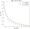 |
Fig. 10. (1 − e) vs M* for the first 2016 XMM observation. |
We expect the star involved in this event to be a WD. The presence of a WD is indeed supported by observations because abundant oxygen has been revealed. Furthermore, the small fraction of accreted mass per orbit (∼10−10) agrees with the hypothesis of a stellar object characterized by high compactness.
The tidal disruption of a WD by an IMBH was considered by Clausen & Eracleous (2011) to explain the broad [O III] line observed in the optical spectra of XMMU J122939.7+075333: by modeling the photoionization of the unbound debris by the accretion flare, its luminosity and width could be very well reproduced, but this possibility was discarded because the timescale expected in case of a full stellar disruption is too short. This limitation, however, is not relevant for the repeating partial disruption that we propose to explain the phenomenology displayed by XMMU J122939.7+075333.
Our results are consistent with those of Zalamea et al. (2010), who investigated the gravitational emission from tidally stripped WDs. They divided the process into two phases: the first phase is longer and characterized by (slow) gravitational wave in-spiraling, while the second phase is shorter and terminates with the detonation of the WD. During the first stage, the periodic mass loss occurring at the pericenter is very small and thus the overall mass of the WD is roughly unchanged. This phase, which is characterized by periodic electromagnetic signals from the system, continues for a number of orbits given by Zalamea et al. (2010) and Shen (2019)
If we apply this estimate to our case, we have 𝒩orb ∼ 7000 orbits, corresponding to ∼25 yr for an orbital period of 112 ks. This timescale is compatible with the time interval over which we observed the recurrent X-ray flares.
Unlike Zalamea et al. (2010), MacLeod et al. (2014) simulated a pTDE of a WD by a massive BH (∼105 M⊙), and they find that this process lasts a few dozen orbits before the full disruption of the star, while according to Zalamea et al. (2010), the process should be much longer. The only way to alleviate this tension is to perform further simulations of this scenario.
We note that the relation between the amount of accreted mass and the penetration factor that we used (Guillochon & Ramirez-Ruiz 2013) is based on numerical simulations of pTDE of main-sequence stars on parabolic orbits7. Although it is the easiest assumption to extrapolate these numbers for the case at hand, a proper set of numerical simulation will be performed in the future to estimate more precisely how the orbital parameters change for the case of interest.
Finally, a curious feature of XMMU J122939.7+075333 is that before 2004, it was always observed in a high-luminosity state. However, after a while, it started to alternate between periods of high luminosity and periods of quiescence. This behavior could be explained assuming that the outer layers of the WD were initially stripped away and were continuously accreted on the BH for some time. The surviving core might then have returned to the pericenter, giving rise to the recurrent flares that we now observe. Another intriguing possibility is that the WD orbit has become wider and/or more eccentric with time, switching from a persistently accreting X-ray binary to a system in which the donor star loses mass only close to periastron. Although this type of evolution is predicted by evolution models of eccentric binaries in which the accretor is more massive than the donor (see, e.g., Dosopoulou & Kalogera 2016), in order to obtain a strong increase in period in only a few dozen years, a more complex scenario might be envisaged (e.g., a third object might drive the orbital evolution through the Kozai–Lidov mechanism; Kozai 1962; Lidov 1962). This hypothesis can be tested by future observations, which might confirm the flare recurrence and its possible increase in frequency with time.
5. Summary and conclusions
The systematic analysis of the X-ray data currently available for the ULX XMMU J122939.7+075333 has allowed us to identify a possibly regular flaring behavior for the first time. The spectral analysis of these X-ray flares suggests that they can be produced by accretion onto a ∼103 M⊙ BH and that the donor star might be oxygen rich. The properties of the peculiar optical counterpart support the latter conclusion and indicate a WD as the likely origin of the accreting matter. We therefore propose that the recurrent flares might be produced by the partial disruption of a WD in a highly eccentric orbit around an IMBH. Being located in a GC, the extreme eccentricity required by our model can originate from the close encounter between the two objects, which might have occurred only a few decades ago, as might be indicated by the higher, possibly persistent luminosity registered in the oldest observations and the gradual reduction of the flare duty cycle in the most recent ones.
This scenario resembles the scenarii that were proposed by many authors (King 2020; Sheng et al. 2021; Arcodia et al. 2021; Chakraborty et al. 2021) to interpret the QPEs that were recently detected in the nuclear regions of galaxies, which very likely host supermassive BHs with relatively low masses (∼105–106 M⊙). If the regular flaring pattern of XMMU J122939.7+075333 were confirmed by future observations, it would be a scaled-down example of the QPE phenomenon in a different environment, but characterized by a similarly high stellar density. We finally note that this peculiar accretion regime might have already been observed in other GC X-ray sources, such as the X9 source at the center of the 47 Tuc GC (Miller-Jones et al. 2015) and several extragalactic X-ray transients (Sivakoff et al. 2005; Jonker et al. 2013; Irwin et al. 2016).
This result is in contrast with Joseph et al. (2015), who reported that only observation 12888 was significantly variable, based on the fit of the light curves with a constant function. If we fit with a constant the 0.5–2 keV background-subtracted light-curve of each observation, binned at 10 ks so that the minimum number of counts per bin permits the application of the χ2 statistic, we obtain unacceptable  values: 4.5 for 13 d.o.f. and 3.2 for 16 d.o.f. for observations 12889 and 12888, respectively.
In addition to the spectra described in the previous section, we extracted the spectra from two different time intervals from the XMM-Newton observation performed in 2004 (Maccarone et al. 2007).
Recently, Wang et al. (2021) have also simulated pTDEs, but assuming stellar BHs, lighter than the one we consider for this work.
Acknowledgments
The scientific results reported in this article are based on observations obtained with XMM-Newton, an ESA science mission with instruments and contributions directly funded by ESA Member States and NASA, and on data obtained from the Chandra Data Archive and has made use of the software package CIAO provided by the Chandra X-ray Center (CXC). We acknowledge the computing centers of INAF (Osservatorio Astronomico di Trieste/Osservatorio Astrofisico di Catania), under the coordination of the CHIPP project, for the availability of computing resources and support. We acknowledge financial support from ASI under ASI/INAF agreement N.2017-14.H.0 A.T. and P.E. acknowledge financial support from the Italian Ministry for University and Research, through grant 2017LJ39LM (UNIAM). M.A.S. acknowledges the Alexander von Humboldt Foundation for the financial support provided in the framework of the research program “The evolution of black holes from stellar to galactic scales”, the Volkswagen Foundation Trilateral Partnership project No. I/97778 “Dynamical Mechanisms of Accretion in Galactic Nuclei”, and the Sonderforschungsbereich SFB 881 “The Milky Way System” – Project-ID 138713538 – funded by the German Research Foundation (DFG).
References
- Arca Sedda, M., Askar, A., & Giersz, M. 2018, MNRAS, 479, 4652 [NASA ADS] [CrossRef] [Google Scholar]
- Arca Sedda, M., Amaro Seoane, P., & Chen, X. 2021a, A&A, 652, A54 [NASA ADS] [CrossRef] [EDP Sciences] [Google Scholar]
- Arca-Sedda, M., Rizzuto, F. P., Naab, T., et al. 2021b, ApJ, 920, 128 [NASA ADS] [CrossRef] [Google Scholar]
- Arcodia, R., Merloni, A., Nandra, K., et al. 2021, Nature, 592, 704 [NASA ADS] [CrossRef] [Google Scholar]
- Bachetti, M., Harrison, F. A., Walton, D. J., et al. 2014, Nature, 514, 202 [NASA ADS] [CrossRef] [Google Scholar]
- Bahramian, A., Heinke, C. O., Tudor, V., et al. 2017, MNRAS, 467, 2199 [Google Scholar]
- Bardeen, J. M., Press, W. H., & Teukolsky, S. A. 1972, ApJ, 178, 347 [Google Scholar]
- Chakraborty, J., Kara, E., Masterson, M., et al. 2021, ApJ, 921, L40 [NASA ADS] [CrossRef] [Google Scholar]
- Clausen, D., & Eracleous, M. 2011, ApJ, 726, 34 [NASA ADS] [CrossRef] [Google Scholar]
- Dage, K. C., Zepf, S. E., Bahramian, A., et al. 2018, ApJ, 862, 108 [NASA ADS] [CrossRef] [Google Scholar]
- Dage, K. C., Zepf, S. E., Bahramian, A., et al. 2019, MNRAS, 489, 4783 [NASA ADS] [CrossRef] [Google Scholar]
- De Luca, A., Salvaterra, R., Belfiore, A., et al. 2021, A&A, 650, A167 [NASA ADS] [CrossRef] [EDP Sciences] [Google Scholar]
- Di Carlo, U. N., Mapelli, M., Pasquato, M., et al. 2021, MNRAS, 507, 5132 [NASA ADS] [CrossRef] [Google Scholar]
- Dosopoulou, F., & Kalogera, V. 2016, ApJ, 825, 71 [NASA ADS] [CrossRef] [Google Scholar]
- Eggleton, P. P. 1983, ApJ, 268, 368 [Google Scholar]
- Garmire, G. P., Bautz, M. W., Ford, P. G., & Nousek, J. A. 2003, X-ray and Gamma-ray Telescopes and Instruments for Astronomy, eds. J. E. Truemper, & H. D. Tananbaum (Bellingham: SPIE), Proc. SPIE, 4851, 28 [NASA ADS] [CrossRef] [Google Scholar]
- Giacconi, R., Branduardi, G., Briel, U., et al. 1979, ApJ, 230, 540 [NASA ADS] [CrossRef] [Google Scholar]
- Giesers, B., Kamann, S., Dreizler, S., et al. 2019, A&A, 632, A3 [NASA ADS] [CrossRef] [EDP Sciences] [Google Scholar]
- Giustini, M., Miniutti, G., & Saxton, R. D. 2020, A&A, 636, L2 [NASA ADS] [CrossRef] [EDP Sciences] [Google Scholar]
- Guillochon, J., & Ramirez-Ruiz, E. 2013, ApJ, 767, 25 [NASA ADS] [CrossRef] [Google Scholar]
- Ingram, A., Motta, S. E., Aigrain, S., & Karastergiou, A. 2021, MNRAS, 503, 1703 [NASA ADS] [CrossRef] [Google Scholar]
- Irwin, J. A., Brink, T. G., Bregman, J. N., & Roberts, T. P. 2010, ApJ, 712, L1 [NASA ADS] [CrossRef] [Google Scholar]
- Irwin, J. A., Maksym, W. P., Sivakoff, G. R., et al. 2016, Nature, 538, 356 [NASA ADS] [CrossRef] [Google Scholar]
- Israel, G. L., Belfiore, A., Stella, L., et al. 2017, Science, 355, 817 [NASA ADS] [CrossRef] [Google Scholar]
- Jonker, P. G., Glennie, A., Heida, M., et al. 2013, ApJ, 779, 14 [NASA ADS] [CrossRef] [Google Scholar]
- Joseph, T. D., Maccarone, T. J., Kraft, R. P., & Sivakoff, G. R. 2015, MNRAS, 447, 1460 [NASA ADS] [CrossRef] [Google Scholar]
- Katz, H., & Ricotti, M. 2013, MNRAS, 432, 3250 [Google Scholar]
- King, A. 2020, MNRAS, 493, L120 [Google Scholar]
- Kozai, Y. 1962, AJ, 67, 591 [Google Scholar]
- Leibowitz, E. 2020, ApJ, 896, 74 [NASA ADS] [CrossRef] [Google Scholar]
- Lidov, M. L. 1962, Planet Space Sci., 9, 719 [NASA ADS] [CrossRef] [Google Scholar]
- Lin, L. C.-C., Hu, C.-P., Li, K.-L., et al. 2020, MNRAS, 491, 5682 [NASA ADS] [CrossRef] [Google Scholar]
- Maccarone, T. J. 2005, MNRAS, 364, 971 [NASA ADS] [CrossRef] [Google Scholar]
- Maccarone, T. J., Kundu, A., Zepf, S. E., & Rhode, K. L. 2007, Nature, 445, 183 [NASA ADS] [CrossRef] [Google Scholar]
- Maccarone, T. J., Kundu, A., Zepf, S. E., & Rhode, K. L. 2010, MNRAS, 409, L84 [NASA ADS] [CrossRef] [Google Scholar]
- MacLeod, M., Goldstein, J., Ramirez-Ruiz, E., Guillochon, J., & Samsing, J. 2014, ApJ, 794, 9 [NASA ADS] [CrossRef] [Google Scholar]
- Metzger, B. D., Stone, N. C., & Gilbaum, S. 2022, ApJ, 926, 101 [NASA ADS] [CrossRef] [Google Scholar]
- Miller-Jones, J. C. A., Strader, J., Heinke, C. O., et al. 2015, MNRAS, 453, 3918 [Google Scholar]
- Miniutti, G., Saxton, R. D., Giustini, M., et al. 2019, Nature, 573, 381 [Google Scholar]
- Morscher, M., Pattabiraman, B., Rodriguez, C., Rasio, F. A., & Umbreit, S. 2015, ApJ, 800, 9 [NASA ADS] [CrossRef] [Google Scholar]
- Motta, S. E., Marelli, M., Pintore, F., et al. 2020, ApJ, 898, 174 [NASA ADS] [CrossRef] [Google Scholar]
- Nandra, K., Briel, D., & Barcons, H. 2013, ArXiv e-prints [arXiv:1306.2307] [Google Scholar]
- Peacock, M. B., Zepf, S. E., Kundu, A., et al. 2012, ApJ, 759, 126 [NASA ADS] [CrossRef] [Google Scholar]
- Pfeffermann, E., Briel, U. G., & Hippmann, H. 1987, Soft X-ray Optics and Technology, eds. E.-E. Koch, & G. Schmahl (Bellingham: SPIE), SPIE Conf. Ser., 733, 519 [Google Scholar]
- Qin, Y., Marchant, P., Fragos, T., Meynet, G., & Kalogera, V. 2019, ApJ, 870, L18 [Google Scholar]
- Rees, M. J. 1988, Nature, 333, 523 [Google Scholar]
- Rhode, K. L., & Zepf, S. E. 2001, AJ, 121, 210 [NASA ADS] [CrossRef] [Google Scholar]
- Ripamonti, E., & Mapelli, M. 2012, MNRAS, 423, 1144 [NASA ADS] [CrossRef] [Google Scholar]
- Rizzuto, F. P., Naab, T., Spurzem, R., et al. 2021a, MNRAS, 501, 5257 [NASA ADS] [CrossRef] [Google Scholar]
- ROSAT Scientific Team 2000, VizieR Online Data Catalog, IX/28A [Google Scholar]
- Saxton, R., Komossa, S., Auchettl, K., & Jonker, P. G. 2020, Space Sci. Rev., 216, 85 [NASA ADS] [CrossRef] [Google Scholar]
- Shen, R.-F. 2019, ApJ, 871, L17 [CrossRef] [Google Scholar]
- Sheng, Z., Wang, T., Ferland, G., et al. 2021, ApJ, 920, L25 [NASA ADS] [CrossRef] [Google Scholar]
- Sivakoff, G. R., Sarazin, C. L., & Jordán, A. 2005, ApJ, 624, L17 [NASA ADS] [CrossRef] [Google Scholar]
- Sniegowska, M., Czerny, B., Bon, E., & Bon, N. 2020, A&A, 641, A167 [NASA ADS] [CrossRef] [EDP Sciences] [Google Scholar]
- Stiele, H., & Kong, A. K. H. 2019, ApJ, 877, 115 [NASA ADS] [CrossRef] [Google Scholar]
- Strüder, L., Briel, U., Dennerl, K., et al. 2001, A&A, 365, L18 [Google Scholar]
- Tully, R. B., Shaya, E. J., Karachentsev, I. D., et al. 2008, ApJ, 676, 184 [Google Scholar]
- Turner, M. J. L., Abbey, A., Arnaud, M., et al. 2001, A&A, 365, L27 [CrossRef] [EDP Sciences] [Google Scholar]
- Wang, Y.-H., Perna, R., & Armitage, P. J. 2021, MNRAS, 503, 6005 [NASA ADS] [CrossRef] [Google Scholar]
- Wilms, J., Allen, A., & McCray, R. 2000, ApJ, 542, 914 [Google Scholar]
- Zalamea, I., Menou, K., & Beloborodov, A. M. 2010, MNRAS, 409, L25 [NASA ADS] [CrossRef] [Google Scholar]
- Zampieri, L., & Roberts, T. P. 2009, MNRAS, 400, 677 [NASA ADS] [CrossRef] [Google Scholar]
- Zepf, S. E., Maccarone, T. J., Bergond, G., et al. 2007, ApJ, 669, L69 [NASA ADS] [CrossRef] [Google Scholar]
- Zepf, S. E., Stern, D., Maccarone, T. J., et al. 2008, ApJ, 683, L139 [NASA ADS] [CrossRef] [Google Scholar]
- Zhao, Z. Y., Wang, Y. Y., Zou, Y. C., Wang, F. Y., & Dai, Z. G. 2021, A&A, submitted [arXiv:2109.03471] [Google Scholar]
All Tables
Best-fit parameters of the EPIC-pn spectra during flares and quiescence in the 2016 XMM-Newton observations.
All Figures
|
Fig. 1. EPIC-pn light curves (from top to bottom: 0.15–0.5 keV, 0.5–1 keV, 1–2 keV, and 2–8 keV) extracted from the source (black) and background (red) regions during the three XMM-Newton observations performed in 2016 (0761630101, 0761630201, and 0761630301). The background count rates (and error bars) are rescaled by a factor 10 to account for the different sizes of the source and background regions. |
| In the text | |
|
Fig. 2. Energy dependence of the peak separation (left panel) and FWHM (right panel) of the three flares observed in the 2016 XMM-Newton observations in three energy bands and in the 0.15–2 keV total range. The separation between the first two flares has been divided by 2 in order to compare it with the separation between the last two flares. |
| In the text | |
|
Fig. 3. ACIS-S light curves (from top to bottom: 0.5–1 keV, 1–2 keV, and 2–8 keV) extracted from the source (black) and background (red) regions during the two Chandra observations performed in 2011 (12888 and 12889). The background count rates (and error bars) are rescaled by a factor of 3 to account for the different sizes of the source and background regions. |
| In the text | |
|
Fig. 4. EPIC-pn light curves in the 0.15–2 keV energy band during observation 0722670601. Top panel: light curve extracted from the source (black squares) and background (red) regions. The background count rates (and error bars) are rescaled by a factor 12 to account for the different sizes of the source and background regions. Bottom panel: background-subtracted light curve. |
| In the text | |
|
Fig. 5. ACIS-S light curve in the 0.3–2 keV energy band extracted from the source (black squares) and background (red) regions during observation 16260. The background count rates (and error bars) are rescaled by a factor 25 to account for the different sizes of the source and background regions. |
| In the text | |
|
Fig. 6. Light curves in the 0.15–2 keV energy band during the 2008 XMM-Newton observation (0510011501). Top panel: EPIC-pn light curve extracted from the source (black squares) and background (red) regions. The background count rates (and error bars) are rescaled by a factor of 10 to account for the different sizes of the source and background regions. Middle panel: EPIC-pn background-subtracted light curve. Bottom panel: EPIC MOS1+MOS2 background-subtracted light curve. |
| In the text | |
|
Fig. 7. EPIC-pn spectra (upper panel) and residuals with respect to the best-fit model with parameters in Table 2 (lower panel) of XMMU J122939.7+075333 in observations 0761630101 (black during flare, red in quiescence), 0761630201 (green during flare, blue in quiescence) and 0761630301 (cyan during flare, purple in quiescence). |
| In the text | |
|
Fig. 8. Time evolution of the power-law 0.3–10 keV unabsorbed luminosity (upper panel), apparent inner disk radius (middle panel; from the diskbb model in XSPEC, assuming a disk inclination of 45°) and Gaussian line flux (lower panel) obtained by fitting the available spectra with the same model as in Table 2. Spectra extracted from the full observation, flare, and quiescent time intervals are represented by black circles, red stars and blue squares, respectively. The time separations between the exposures performed during the same year have been enhanced for clarity. |
| In the text | |
|
Fig. 9. Light curves and 3σ upper limits of XMMU J122939.7+075333 in luminosity units for all the XMM-Newton and Chandra observations in Table 1. The conversion from 0.5–2 keV count rates into luminosity in the 0.5–2 keV energy band was based on the best-fit parameters of the average spectrum for each observation. The upper limits were derived from the 0.3–2 keV count-rate limits in Table 1 assuming the best-fit spectral parameters of the first flare detected in 2016 (Table 2). Although Dage et al. (2019) report a 3σ detection in the 2019 observation, we set an upper limit because most of the counts were detected above 2 keV. The horizontal bars indicate either the bin size of the light curve (ranging from 1 to 10 ks) or the observation exposure time (for upper limits and observations with a single time bin). The start dates of the observations and the instrument are indicated in each panel. |
| In the text | |
|
Fig. 10. (1 − e) vs M* for the first 2016 XMM observation. |
| In the text | |
Current usage metrics show cumulative count of Article Views (full-text article views including HTML views, PDF and ePub downloads, according to the available data) and Abstracts Views on Vision4Press platform.
Data correspond to usage on the plateform after 2015. The current usage metrics is available 48-96 hours after online publication and is updated daily on week days.
Initial download of the metrics may take a while.