| Issue |
A&A
Volume 661, May 2022
The Early Data Release of eROSITA and Mikhail Pavlinsky ART-XC on the SRG mission
|
|
|---|---|---|
| Article Number | A7 | |
| Number of page(s) | 17 | |
| Section | Cosmology (including clusters of galaxies) | |
| DOI | https://doi.org/10.1051/0004-6361/202142462 | |
| Published online | 18 May 2022 | |
The eROSITA Final Equatorial-Depth Survey (eFEDS)
X-ray properties and scaling relations of galaxy clusters and groups★
1
Max Planck Institute for Extraterrestrial Physics,
Giessenbachstrasse 1,
85748
Garching, Germany
e-mail: This email address is being protected from spambots. You need JavaScript enabled to view it.
2
IRAP, Université de Toulouse, CNRS, UPS, CNES,
Toulouse, France
3
Argelander-Institut für Astronomie (AIfA), Universität Bonn,
Auf dem Hügel 71,
53121
Bonn, Germany
4
Tsung-Dao Lee Institute, and Key Laboratory for Particle Physics, Astrophysics and Cosmology, Ministry of Education, Shanghai Jiao Tong University,
Shanghai
200240, PR China
5
Universitaets-Sternwarte Muenchen, Fakultaet fuer Physik, LMU Munich,
Scheinerstr. 1,
81679
Munich, Germany
6
Physics Program, Graduate School of Advanced Science and Engineering, Hiroshima University,
1-3-1 Kagamiyama, Higashi-Hiroshima,
Hiroshima 739-8526, Japan
7
Hiroshima Astrophysical Science Center, Hiroshima University,
1-3-1 Kagamiyama, Higashi-Hiroshima,
Hiroshima 739-8526, Japan
8
Core Research for Energetic Universe, Hiroshima University,
1-3-1, Kagamiyama, Higashi-Hiroshima,
Hiroshima 739-8526, Japan
Received:
15
October
2021
Accepted:
16
December
2021
Abstract
Context. Scaling relations link the physical properties of clusters at cosmic scales. They are used to probe the evolution of large-scale structure, estimate observables of clusters, and constrain cosmological parameters through cluster counts.
Aims. We investigate the scaling relations between X-ray observables of the clusters detected in the eFEDS field using Spectrum-Roentgen-Gamma/eROSITA observations taking into account the selection effects and the distributions of observables with cosmic time.
Methods. We extract X-ray observables (LX, Lbol, T, Mgas, YX) within R500 for the sample of 542 clusters in the eFEDS field. By applying detection and extent likelihood cuts, we construct a subsample of 265 clusters with a contamination level of <10% (including AGNs and spurious fluctuations) to be used in our scaling relations analysis. The selection function based on the state-of-the-art simulations of the eROSITA sky is fully accounted for in our work.
Results. We provide the X-ray observables in the core-included <R500 and core-excised 0.15 R500-R500 apertures for 542 galaxy clusters and groups detected in the eFEDS field. Additionally, we present our best-fit results for the normalization, slope, redshift evolution, and intrinsic scatter parameters of the X-ray scaling relations between LX - T, LX - Mgas, LX - YX, Lbol - T, Lbol - Mgas, Lbol - YX, and Mgas - T. We find that the best-fit slopes significantly deviate from the self-similar model at a >4σ confidence level, but our results are nevertheless in good agreement with the simulations including non-gravitational physics, and the recent results that take into account selection effects.
Conclusions. The strong deviations we find from the self-similar scenario indicate that the non-gravitational effects play an important role in shaping the observed physical state of clusters. This work extends the scaling relations to the low-mass, low-luminosity galaxy cluster and group regime using eFEDS observations, demonstrating the ability of eROSITA to measure emission from the intracluster medium out to R500 with survey-depth exposures and constrain the scaling relations in a wide mass-luminosity-redshift range.
Key words: galaxies: clusters: general / galaxies: groups: general / galaxies: clusters: intracluster medium / X-rays: galaxies: clusters
The lists of best-fit electron density model parameters (Table 1) of eFEDS clusters and X-ray observable measurements (Table 2) are available at the CDS via anonymous ftp to cdsarc.u-strasbg.fr (130.79.128.5) or via http://cdsarc.u-strasbg.fr/viz-bin/cat/J/A+A/661/A7 or can be found at https://erosita.mpe.mpg.de/edr/eROSITAObservations/Catalogues
© Y. Emre Bahar et al. 2022
 Open Access article, published by EDP Sciences, under the terms of the Creative Commons Attribution License (https://creativecommons.org/licenses/by/4.0), which permits unrestricted use, distribution, and reproduction in any medium, provided the original work is properly cited.
Open Access funding provided by Max Planck Society.
1 Introduction
Galaxy clusters, which are formed by the gravitational collapse of the largest density peaks in the primordial density field, represent the largest virialized objects in the Universe. Embedded in the cosmic web, they evolve and grow through mergers and by accreting smaller subhaloes via the surrounding large-scale structure (e.g., Kravtsov & Borgani 2012). The number counts of clusters of galaxies as a function of redshift and their mass is a powerful cosmological probe that is orthogonal and complementary to other cosmological geometrical experiments (e.g., Pillepich et al. 2012; Mantz et al. 2015; Schellenberger & Reiprich 2017; Pacaud et al. 2018, also see Pratt et al. 2019 for a review). Additionally, based on the current Lambda cold dark matter (ACDM) cosmological model, galaxy clusters are among the structures formed last, and therefore capture the formation history and the growth of the structure in the Universe.
Well-established scaling relations between cluster mass and observables provide a way forward for cosmological investigations using clusters of galaxies. Accurate estimates of cluster total masses are crucial ingredients for exploiting the cluster number counts as cosmological probes. However, measurements of masses of individual clusters through multi-wavelength (X-ray, optical, weak lensing, and radio) observations can be expensive for larger cluster samples. Scaling relations aid this problem and bridge cluster number counts with cosmology. On the other hand, the scaling relations between observables and their evolution allow us to constrain intracluster medium (ICM) physics and theoretical models based on gravitational collapse (e.g., Kaiser 1986; Ascasibar et al. 2006; Short et al. 2010; Capelo et al. 2012). Kaiser (1986) modeled the formation of clusters as scale-free collapses of initial density peaks and derived relations between ICM properties that result in clusters at different red-shifts and masses being scaled versions of each other. This is called the self-similar model in the literature. Other nongravi-tational physical processes, such as radiative cooling, galactic winds, turbulence, and AGN feedback, that affect the formation and evolution of these objects throughout cosmic time may have imprints on these relations. In observational studies, these imprints are quantified by measuring deviations from the self-similar scaling relations. Clusters of galaxies owing to their deep potential well are less prone to these nongravitational processes, while the intra-group gas in galaxy groups can be significantly impacted by nongravitational physics (e.g., Tozzi & Norman 2001; Borgani et al. 2002; Babul et al. 2002; Puchwein et al. 2008; Biffi et al. 2014; Barnes et al. 2017).
The majority of the baryonic content of the clusters is in the form of X-ray-emitting hot ionized plasma, the ICM. Being in the fully ionized state and reaching up to 108 Kelvin in temperature, the ICM emits primarily in X-rays through thermal Bremsstrahlung, offering an opportunity to measure physical properties of the ICM, to establish scaling relations between these properties and mass, and to constrain their evolution over cosmic time. The scaling relations between X-ray observables and mass have been extensively explored for massive clusters in the literature, selected in various ways by the large-area, multi-wavelength surveys (e.g., Mantz et al. 2010b; Bulbul et al. 2019). However, samples including a sufficient number of uniformly selected groups covering the low-mass, low-redshift, and low-luminosity range with adequate count rates are limited. Studies of the scaling relations of galaxy groups and clusters spanning a wide mass, luminosity, and redshift range with large-area surveys with a well-understood selection will improve our understanding of the interplay between galaxy evolution, AGN feedback, and gravitational processes in these deep potential wells. XMM-Newton’s largest observational programme XXL (Pierre et al. 2011) served as a bridge between narrow and deep observations (e.g., CDF-S, Finoguenov et al. 2015) and very wide, moderately deep observations (e.g., RASS, Ebeling et al. 1998) by populating the intermediate parameter space with detected clusters. Most recently, the extended ROentgen Survey with an Imaging Telescope Array (eROSITA, Merloni et al. 2012; Predehl et al. 2021) carried out its eROSITA Final Equatorial-Depth Survey (eFEDS) observations and provided numerous cluster detections that span a large mass–redshift space. eROSITA on board the Spectrum-Roentgen-Gamma (SRG) mission continues to detect large numbers of clusters spanning a wide range of redshift and mass since its launch in 2019. It will provide sufficient statistical power and place the tightest constraints on these scaling relations for probing their mass and redshift evolution.
The eFEDS was performed during eROSITA’s calibration and performance verification phase (Predehl et al. 2021; Brunner et al. 2022; Liu et al. 2022a). eFEDS, the first (mini)survey of eROSITA, is designed to serve as a demonstration of the observational capabilities of the telescope to the scientific community. The survey area is located at (approximately) 126° < RA < 146° and −3° < Dec < +6° and covers a total of ~140 deg2. The exposure time of the survey area is mostly uniform with average vignetted and unvignetted exposure times of ~1.3 and ~2.2 ks, respectively (Brunner et al. 2022). The eFEDS area is also covered in survey programs of other telescopes such as the Hyper Supreme-Cam Subaru Strategic Program (HSC-SSP; Aihara et al. 2018), DECaLS (Dark Energy Camera Legacy Survey, Dey et al. 2019), SDSS (Sloan Digital Sky Survey, Blanton et al. 2017, Ider-Chitham et al., in prep.), 2MRS (2MASS Redshift Survey, Huchra et al. 2012), and GAMA (Galaxy And Mass Assembly, Driver et al. 2009). These observations are used to optically confirm the detected clusters and measure their redshifts (Klein et al. 2022, Ider-Chitham et al., in prep.). In addition to the optical confirmation and redshift determination, HSC-SSP observations are also used in measuring the weak lensing mass estimates of the detected clusters. The observables presented in this work are measured using R5001 values inferred from these weak lensing measurements (Chiu et al. 2022). In this work, we provide X-ray properties of the 542 galaxy clusters and groups in the full eFEDS-extent-selected sample in two apertures (r < R500 and 0.15 R500 < r < R500) (Liu et al. 2022a). Additionally, we investigate the scaling relations between core-included (r < R500) X-ray observables in a subsample of 265 galaxy clusters and groups with a lower level of contamination by noncluster detections. This work expands the scaling relation studies to the poorly explored mass (6.86 × 10¹² M⊙ < M500 < 7.79 × 10¹⁴ M⊙), luminosity (8.64 × 1040 erg s−1 < LX < 3.96 × 1044 erg s−1), and redshift (0.017 < z < 0.94) ranges with the largest number of galaxy groups and clusters, paving the way for similar studies using the eROSITA All-Sky survey (eRASS) observations. We note that the scaling relations between X-ray observables and weak lensing masses have already been published in our companion paper, Chiu et al. (2022). The selection function is based on the realistic full sky simulations of eROSITA and is fully accounted for in our results (Comparat et al. 2020). Throughout this paper, the best-fitting thermal plasma temperature to the cluster spectra is marked with T, LX stands for soft-band X-ray luminosity calculated in the 0.5–2.0 keV energy band, Lbol stands for the bolometric luminosity calculated in the 0.01–100 keV energy band, the errors correspond to 68%, and we adopt a flat ACDM cosmology using the Planck Collaboration XIII (2016) results, namely Ωm = 0.3089, σ8 = 0.8147, and H0 = 67.74 km s−1 Mpc−1.
2 Data analysis
2.1 Data reduction and sample selection
The eFEDS observations were performed by eROSITA between 4 and 7 November 2019. The observation strategy allowed the eFEDS field to be surveyed nearly uniformly with a vignetted exposure of ~1.3 ks which is similar to the expected vignetted exposure of the final eROSITA All-Sky Survey (eRASS8) at the equatorial regions. Initial processing of the eFEDS observations was carried out using the eROSITA Standard Analysis Software System (eSASS, version eSASSusers_201009, Brunner et al. 2022). In this paper, we only present an outline of the summary of the data reduction and source detection. We refer the reader to Brunner et al. (2022) and Liu et al. (2022a) for a more detailed explanations of these steps. We first applied filtering to X-ray data, removing dead time intervals and frames, corrupted events, and bad pixels. Images created in the 0.2–2.3 keV band using all available telescope modules (TMs) are passed to eSASS source-detection tools in order to perform the source detection procedure and provide extension and detection likelihoods. After applying a detection likelihood (ℒdet) threshold of 5 and an extension likelihood (ℒext) threshold of 6, we obtained 542 cluster candidates in the eFEDS field (Brunner et al. 2022). The physical properties of these clusters, such as soft-band and bolo-metric luminosities, and ICM temperature measurements within a physical radius of 300 and 500 kpc are provided by Liu et al. (2022a).
We used realistic simulations of the eFEDS field (Liu et al. 2022b) in order to measure the contamination fractions of samples with different ℒdet and ℒext cuts. According to these simulations, the eFEDS cluster catalog, which consists of 542 clusters, has a contamination fraction of ~20%. This is a relatively high contamination rate for statistical studies. In order to avoid significant bias caused by the noncluster sources present in the sample (e.g., AGNs and spurious sources), we applied ℒdet > 15 and ℒext > 15 cuts that give us a sample of 265 clusters with an expected contamination fraction of 9.8%. The final sample covers a total mass range of (6.86 × 10¹² M⊙ < M500 < 7.79 × 10¹⁴ M⊙, a luminosity range of 8.64 × 1040 erg s−1 < Lx < 3.96 × 1044 erg s−1, and a redshift range of (0.017 < z < 0.94). The redshift and mass histograms of this final subsample are shown in Fig 1. Consisting of 68 low-mass (<1014 M⊙) galaxy groups, this work extends the scaling relation studies to the low-mass range with one of the largest group samples detected uniformly to date.
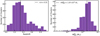 |
Fig. 1 Left: redshift histogram of the ℒdet > 15, ℒext > 15 sample used in this work. Right: weak lensing calibrated total mass |

2.2 X-ray observables within R500
One of the main goals of this paper is to provide X-ray properties of eFEDS clusters within the overdensity radius of R500-Here we provide a short summary of the methods we employed to extract X-ray observables. For a complete description, we refer the reader to Ghirardini et al. (2021) and Liu et al. (2022a).
The measurements of R500 used in this work are obtained from the weak lensing calibrated cluster masses presented in our companion paper (Chiu et al. 2022). Calibration is applied by using the eFEDS observations of the same cluster sample used in this work which enables the R500 measurements to be self-consistent. Mass estimates are obtained by jointly modeling the eROSITA X-ray count-rate (η) and HSC shear profile (g+) as a function of cluster mass (M500) and obtaining a scaling relation between η − m500 − z. After obtaining the mass estimates, R500 measurements are calculated by 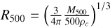 where ρc is the critical density at a given redshift and cosmology. We refer the reader to Chiu et al. (2022) for a more detailed description of the HSC weak-lensing mass calibration analysis.
X-ray spectra of clusters are extracted within R500, both core-included (r < R500) and core-excised (0.15R500 < r < R500), using the eSASS code srctool. The background spectra are extracted from an annular region that is 4–6 R500 away from the clusters’ centroid. We fit the X-ray spectra with an absorbed apec thermal plasma emission model (Smith et al. 2001; Foster et al. 2012) to represent the ICM emission. The fitting band of 0.5–8 keV was used for TMs 1, 2, 3, 4, and 6 and a more restricted band of 0.8–8 keV was used for TMs 5 and 7 in the spectral fits due to the light leak noticed during the commissioning phase (see Predehl et al. 2021). The Galactic hydrogen absorption is modeled using tbabs (Wilms et al. 2000), where the column density nH used is fixed to nH,tot,tot (Willingale et al. 2013), estimated at the position of the cluster center. The metallicity of the clusters is fixed to 0.3 Z⊙, adopting the solar abundance table of Asplund et al. (2009). The background spectra and spectra are simultaneously fit to account for the background in the total spectra as described in detail by Ghirardini et al. (2021). The background spectra are modeled with a set of apec and power-law models representing instrumental background based on the filter-wheel closed data (see Freyberg et al. 2020)2, cosmic background (local bubble, galactic halo, and emission from unresolveds AGNs). The best-fit values and standard deviations of the ICM temperatures (T) are measured using the Markov chain Monte Carlo (MCMC) method within XSPEC (version 12.11.0k).
We extract images and exposure maps in the 2.5–2.2 keV energy band to obtain cluster density profiles. We model the two-dimensional distribution of photons by projecting the Vikhlinin et al. (2006) density model. Point sources are either modeled or masked depending on their fluxes; see Ghirardini et al. (2022) for further details. The cosmic background contribution is added to the total model as a constant. The resulting total image is finally convolved with eROSITA’s vignetted exposure map, while the instrumental background model is folded with the unvignetted exposure map. A Poisson log-likelihood in MCMC is used to estimate best-fit cluster model parameters. Finally, the electron density (ne) profile of the gas is obtained by measuring the emissivity using the temperature information recovered from the spectral analysis. Best-fit parameters of clusters to the Vikhlinin et al. (2006) electron density profile model are presented in Table 1. In order to obtain luminosity profiles, LX(r) and Lbol(r), we calculated conversion factors from count rate to luminosity in soft (2.5–2.2 keV) and bolometric (2.21–122 keV) energy bands.
The gas mass (or ICM mass) of the clusters enclosed within R522 is computed by integrating the gas electron density assuming spherical symmetry:
 (1)
(1)
where ne is the number density of electrons, mp is the proton mass, and µe = 1.1548 is the mean molecular weight per electron calculated using the Asplund et al. (2009) abundance table (Bulbul et al. 2010). Lastly, YX is calculated by multiplying the gas mass (Mgas) with the gas temperature (T) as
 (2)
(2)
which is introduced by Kravtsov et al. (2006) as a low scatter mass estimator.
We note that in our analysis, uncertainties in R500 measurements are fully propagated using the MCMC chains and the redshift errors are neglected. We use the single temperature in our calculations as the survey data do not have sufficient depth to recover the temperature profiles as a function of radius. For all eFEDS clusters, we provide the core-included (r < R500) X-ray observables within R500, including T, LX, Lbol, Mgas, and YX as well as the core-excluded X-ray observables extracted between 2.15 R500 − R500 (Tcex, Lx,cex, Lboi,cex) in Table 2. eROSITA’s field-of-view-averaged point spread function (PSF) half-energy width is ~26″ which is comparable to the cores (2.15 R500) of the majority of clusters. This has a mild effect on the LX,cex measurements because we deconvolve the surface brightness profiles with the PSF and use the best-fit core-included temperatures for the emissivity. However, given the limited photon statistics, only a first-order PSF correction is applied to the Tcex measurements where the flux changes at different energies are compensated by assuming the spectrum to be similar over the whole of the source. Therefore, we advise the reader to approach Tcex measurements with caution.
In this work, we focus on the scaling relations between X-ray observables, namely L − T, L − Mgas, L − YX, and Mgas − T. The scaling relations between observables and cluster mass (M500) obtained from weak-lensing observations are already provided in the companion paper by Chiu et al. (2022). Although we provide measurements of the core-excluded observables in this paper in Table 2, we only use the core-included observables in our further analysis for the scaling relations. The reasons for this are twofold, and are related to the selection function, and the decrease in the statistics. Our selection function is built using the core-included observables from the simulations of eROSITA sky (Comparat et al. 2020). Constructing selection functions with the core-excised observables relies on modeling the PSF accurately in simulations. Our imaging analysis and spectral fits account for the PSF spilling,but this analysis is not available yet in simulations. As a workaround, one could model the relation between the core-excised and core-included observables (e.g., P(YX,cex|YX)), but a significant fraction of eFEDS clusters populate a previously poorly explored parameter space and such an approach requires a good understanding of the surface brightness profiles of these clusters. Secondly, when the core is excised, the temperature measurements become either loose or lost due to the decrease in photon statistics. This affects the reliability of the X-ray observable measurements used in our fits and may lead to biased constraints on the scaling relations. A full analysis with the core-excised observables will be carried out for the clusters detected in the eRASS observations, where we expect to have a larger sample of clusters with a higher depth around the ecliptic poles (Ghirardini et al., in prep.).
X-ray best fitting parameters for Vikhlinin et al. (2006) model:  .
.
X-ray observables of eFEDS clusters measured within R500 and between 0.15R500 − R500.
3 Modeling and fitting of the scaling relations
We model the scaling relations and the likelihoods for different pairs of observables in a similar manner with minor tweaks. Therefore, in this section, we present the general form of the scaling relations and the structure of the likelihood for two hypothetical observables: X and Y.
3.1 General form of the scaling relations
Kaiser (1986) derived simple forms of scaling relations, namely self-similar relations, by assuming gravitational interactions to be the driving force of the evolution of groups and clusters. These relations suggest that the observables of clusters follow these simple power-law relations. Departures from these relations are often interpreted as a result of non-gravitational physical processes, such as radiative cooling, galactic winds, and AGN feedback that can have a significant impact on the distribution of baryons in the ICM and energy budget of the system (Bhattacharya et al. 2008; McCarthy et al. 2010; Fabjan et al. 2010; Bulbul et al. 2016; Giodini et al. 2013; Lovisari et al. 2020).
In this work, we use a relation that takes into account the power-law dependence and the redshift evolution of the form
 (3)
(3)
where Ypiv, Xpiv, and zpiv are the pivot values of the sample, and A, B, and C are the normalization, power-law slope, and redshift evolution exponent, respectively. The redshift evolution is modeled using the evolution function which is defined as E(z) = H(z)/H0 where H(z) is the Hubble-Lemaître parameter and H0 is the Hubble constant.
3.2 Likelihood
In our fits to the scaling relations, we take into account various observational and physical effects by adding the relevant components to the corresponding likelihood function similar to the method presented in Giles et al. (2016) for the XXL clusters. The joint probability function in terms of the measured values  of the true values of the observables X and Y is given by
 (4)
(4)
where P(I|Y, z), also known as the selection function, is the probability of a cluster being included (I) in our sample,  is the two-dimensional measurement uncertainty, P(Y|X, θ, z) is the modeled Y − X relation, and the P(X|z) term is the cos-mological distribution of the observable X. The variable θ in the scaling relation term marks the free parameters of the scaling relation, such as A, B, C, and the scatter σY|X. We note that in this work, correlations between the measurement uncertainties of observables X and Y are fully considered using the MCMC chains. We also note that the cosmological parameters are frozen throughout our analysis. More than 65% of the clusters in our sample have spectroscopic redshifts and the remaining clusters have photometric redshift measurements using the high signal-to-noise-ratio HSC data, which provides uncertainties of the order of 03% (see Klein et al. 2022, Ider-Chitham et al., in prep.). Therefore, we assume that the errors on the redshifts have negligible effects on our measurements, that is,
  . The variance in exposure time due to the overlapping regions and the missed observations due to malfunctions of telescope modules (TMs) (see Brunner et al. 2022, for details) are accounted for by using the exposure time (texp) at the X-ray center of each cluster when calculating P(I|Y, z).
We model the Y − X relation such that the observable Y is distributed around the power-law scaling relation log-normally. Assumption of the log-normal distribution of X-ray observables is widely used in the literature (e.g., Pacaud et al. 2007; Giles et al. 2016; Bulbul et al. 2019; Bocquet et al. 2019). The scaling relation term P(Y|X, θ, z) in Eq. (4) then becomes
 (5)
(5)
To obtain the cosmological distribution of the observable X (P(X|z)), that is, the expected distribution of X as a function of redshift given a fixed cosmology and an assumed X − M scaling relation, we convert the Tinker et al. (2008) mass function to a Tinker X function using the Chiu et al. (2022) weak-lensing mass-calibrated scaling relations obtained from the same cluster sample consistently. This conversion is applied such that the intrinsic scatter of the X − M relation is taken into account by the following equation:
 (6)
(6)
where θWL is the best-fit result of the weak-lensing mass-calibrated scaling relation X − M500. We note that the form of the X − M relation presented in Chiu et al. (2022) is different than the form we use in our Y − X relation. Hereafter, we do not include the θWL term in P(X|θWL, z), because it is fixed throughout the analysis. After properly defining all the terms in the joint distribution in Eq. (4), we marginalize over the nuisance variables (X, Y) in order to get the likelihood of obtaining the measured observables  . The final likelihood of a single cluster then becomes
 (7)
(7)
To avoid significant bias in the results due to the assumed cosmological model and the exact form of the X − M relation, we do not use the observed number of detected clusters as data, but instead we take it as a model parameter. In the Bayesian framework, this corresponds to using a likelihood that quantifies the probability of measuring  ; and
; and  observables given that the cluster is detected. Such a likelihood can be obtained using the Bayes theorem where the likelihood for the ith cluster becomes
 (8)
(8)
Lastly, the overall likelihood of the sample is obtained by multiplying the likelihoods of all clusters
 (9)
(9)
where  and
and  are the measurement observables of all clusters in the sample and
  is the number of detected clusters in our sample.
This form of the likelihood is similar to those used in the literature; see for example Mantz et al. (2010a). The most fundamental difference is the goal of this work, which is to fit the scaling relations at a fixed cosmology rather than simultaneously fitting scaling relations and cosmological parameters. Using this likelihood allows us to avoid including terms that have a strong dependence on cosmology, such as those in Mantz et al. (2010b), namely the probability of not detecting the model-predicted, undetected clusters,  , possible ways of selecting
  clusters from the total sample
  , and the prior distribution of the total number of clusters in the field, P(N) (see Mantz 2019, for the use of these parameters). Another benefit of using this likelihood is it allows the results to be less sensitive to the accuracy of the normalization of the X − M relation and therefore makes our analysis more robust for the goal of this work.
3.3 Modeling the selection function
The selection function model adopted here, P(I|Y, z) in Eq. (7), is similar to that described in Liu et al. (2022a). It relies on multiple mock realizations of the eFEDS field (Liu et al. 2022b). The simulations faithfully reproduce the instrumental characteristics of eROSITA and features induced by the scanning strategy (exposure variations, point-spread function, effective area, and the grasps of the seven telescopes.) Realistic foreground and background source models are associated with a full-sky light-cone N-body simulation assuming the Planck-CMB cosmology. These sources include stars, active galactic nuclei (AGN), and galaxy clusters. The method to associate AGN spectral templates to sources is derived from abundance-matching techniques. For clusters and groups, the association between a massive dark matter halo and an emissivity profile drawn from a library of observed templates depends on the mass, redshift, and dynamical state of the halo. In particular, relaxed halos are associated with gas distributions with higher central projected emission measures. The steps leading to the AGN and cluster simulations are extensively described in Comparat et al. (2019, 2020). The SIXTE engine (Dauser et al. 2019) serves in converting sources into event lists, while the eSASS software (Brunner et al. 2022) is used to process those lists and to deliver source catalogs.
The next steps are identical to those in Liu et al. (2022a), except for the definition of an extended detection which assumes ℒdet > 15 and ℒext > 15. In particular, pairs of the simulated and detected sources are looked for in the plane of the sky, accounting for their relative positions, their extents, and favoring association between bright sources in cases of ambiguity. Securely identified matches are flagged as a successful detection.
The modeling of the detection probabilities involves interpolation across the multi-dimensional parameter space describing galaxy cluster properties, which includes their intrinsic soft-band or bolometric luminosity, their redshift, the local exposure time, and optionally the central emission measure. Other parameters are marginalized over, making the assumption that their distributions are correctly reflected in the simulations. To this end, we make use of Gaussian Process classifiers, a class of non-parametric models which capture the variations of the detection probability under the assumption that the covariance function (kernel) is a squared exponential function. One advantage of using such models rather than the multi-dimensional spline interpolation, for example, is a more appropriate mathematical treatment of uncertainties, particularly in poorly populated areas of the parameter space. Two-thirds of the simulated clusters are used for training the classifiers, and the remaining third provides the material to test the performance of the classifiers and to assess their behavior on a realistic population of halos.
In particular, we check that systems assigned a given detection probability by the classifier display a detection rate with a value close to that probability; in such cases the classifier is said to be well-calibrated.
These models are designed to emulate the whole chain of computationally expensive steps needed in performing an eFEDS end-to-end simulation (Liu et al. 2022b). It is worth noting that such selection functions have a range of applicability that is set by the simulation.
In order to demonstrate the representativeness of the selection function, we model the luminosity distribution of the ℒdet > 15, ℒext > 15 clusters and compare it with the observed cluster distribution. We model it as P(I,Lx,z) = P(I|LX, z)P(Lx|z)P(z) where we calculate P(Lx|z) using Eq. (6) and the best-fit LX− M relation presented in Chiu et al. (2022). For the redshift distribution, we assume the comoving cluster density to be constant within our redshift span (0 < z < 0.9) so that P(z) is proportional to the comoving volume shell  (Hogg 1999) where c is the light speed, H0 is the Hubble constant, dA(z) is the angular diameter distance, and Ωs is the solid angle of the eFEDS survey. A comparison between the distribution of the luminosity measurements for the cluster sample with ℒdet > 15, ℒext > 15 selection and our model predicted by our selection function is shown in Fig. 2. The figure visually demonstrates the consistency of the luminosity distribution with redshift predicted from the selection function (plotted as the background color), and measurements from the eFEDS data (white data points and white contours).
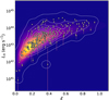 |
Fig. 2 Soft band (0.5–2.0 keV) X-ray luminosity and redshift measurements of the clusters in the eFEDS field that satisfies the ℒdet > 15 and ℒext > 15 condition. Luminosities are measured within apertures of R500- White solid curves are smoothed contours of the Lx − z data points and the color is proportional to the PDF of the hypothetical Lx − z distribution modeled as P(I,Lx,z) = P(I|Lx,z)P(Lx|z)P(z) (see Sect. 3.3 for the description of the model). |
3.4 Fitting
We fit scaling relations using the MCMC sampler package emcee (Foreman-Mackey et al. 2013) with a likelihood described in Sect. 3.2. Before we fit the real data, we validate our fitting code on simulated clusters. For the tests, we mock X-ray observables of a sample of 265 clusters corresponding to the same number of clusters in the sample selected with the criteria of ℒdet > 15 and ℒext > 15. Using the observed redshifts as priors, we sample the observables, X and Y, from a bivariate distribution of the form
 (10)
(10)
where P(Y|X, θsim, z) is the scaling relation term including intrinsic scatter and θsim is the input scaling relation parameters for the simulated clusters. We then scatter the X and Y observables to mimic observational uncertainty and assign conservative error bars to model our observable measurements. We then run our fitting code on the simulated clusters with 100 walkers for 10 000 steps and compare the best-fit θ values with the input parameters (θsim). We find that the fitting code successfully recovers all input parameters with a deviation within one sigma validating the performance and the accuracy of the code.
After the test run, we fit the X-ray scaling relations using the eFEDS measurements using flat priors for all scaling relation parameters;  for the normalization (A),
  for the slope (B),
  for the redshift evolution exponent (C), and
  for the scatter (σY|X). The median values of the observables are used as the pivot values in our fits and are provided in Table 3.
In total, we perform two fits for each scaling relation. The first fits are performed with free redshift evolution exponents, C, and in the second fits the parameter C is fixed to the self-similar values. The self-similar expectations are given in Table 4 for all scaling relations used in this work. The best-fit parameters of these seven relations can be found in Table 5. We provide our results and comparisons with the literature in Sect. 4.
Median values of observables measured for the ℒdet > 15, ℒext > 15 clusters.
Self-similar expected model parameter values of scaling relations of the form  .
.
Best-fit parameters of the scaling relations.
4 Results
Scaling relations between X-ray observables are tools for understanding the ICM physics for various mass scales and evolution of the ICM with redshift, while the relations between observables and cluster mass are used for facilitating cosmology with cluster number counts. In this section we examine the L − T, L − Mgas, L − YX, and Mgas − T scaling relations, using both Lx and Lbol, and provide extensive comparisons with the literature. Owing to the high soft-band sensitivity of the eROSITA, we were able to include a large number of low-mass, low-luminosity clusters in our study, down to the soft band luminosities of 8.64 × 1040 ergs s−1 and masses (M500) of 6.86 × 10¹² M⊙. In the eFEDS field alone, we detect a total of 68 low-mass groups with M500 < 1014 M⊙ that are fully included in our analysis. eROSITA will be revolutionary in both ICM studies and cosmology in this regard as it will extend cluster samples to much lower luminosities and lower masses than ever reached before. We first describe our method and lay the groundwork with the eFEDS sample with this work, and will push the mass and luminosity limits down with our ongoing work on the eRASSl sample. One other important aspect is the fact that the eROSITA group and cluster samples are uniformly selected and the selection function is well understood with the help of our full-sky eROSITA simulations.
There are several complications in comparing scaling relation results in the literature with our results. These are linked to the form of the fitted scaling relations, the energy band of the extracted observables, and the assumed cosmology, and the instrument calibration also varies from one study to another. To overcome these difficulties, we apply corrections before we compare them with our results. In these comparison plots, we use the self-similar redshift evolution as the common reference point and convert the observables accordingly. The standard energy band we use in this paper for the extraction of observables is the 0.5−2.0 keV band. To convert normalizations of scaling relations involving luminosities obtained in the 0.1–2.4 keV energy band (L01−2.4), we faked an unabsorbed APEC spectrum within XSPEC and calculated a conversion factor of 1.64 for a cluster that has a temperature of 3.26 keV, an abundance of 0.3, and a redshift of 0.33. These redshift and temperature values are the median values of our sample (see Table 3). Changing the temperatures and redshifts affects the conversion factor by a few percent, which is consistent with the findings of Lovisari et al. (2020). We therefore applied the same conversion factor to all other works using the 0.1–2.4 keV energy band. Lastly, we convert the relations assuming a dimensionless Hubble constant of 0.6774 which is the value we use in this work. The corrections are only applied to the normalizations, and therefore the slopes and redshift evolution exponents of previously reported relations remain unchanged.
Another challenge in comparisons of scaling relations involving the ICM temperature is the calibration differences between various X-ray telescopes. It has been shown that calibration differences between Chandra and XMM-Newton are dependent on the energy band and can be as large as a factor of two for hot clusters with temperatures >10 keV in the soft band (0.7−2 keV) (Schellenberger et al. 2015). However, this difference is small, namely of 10–15% in the full 0.7−7 keV band for low-temperature clusters (<4 keV) to which we are sensitive in the eFEDS observations. Our preliminary calibration studies with eROSITA showed that, in general, eROSITA temperatures are in good agreement with Chandra and XMM-Newton temperatures (Sanders et al. 2022; Veronica et al. 2022; Iljenkarevic et al. 2022; Whelan et al. 2021). Turner et al. (2021) recently cross-matched the eFEDS cluster catalog (Liu et al. 2022a) with the XMM-Newton Cluster Survey (XCS, Romer et al. 2001) sample and found luminosities of 29 cross-matched clusters to be in excellent agreement. They also compared the temperatures of 8 clusters that are measured with both telescopes and found XMM measurements to have slightly higher temperatures on average. In order to better understand the instrumental differences, more extensive studies should be performed with a cluster sample containing a larger range of temperatures using the survey data. This will be further investigated in future eROSITA projects.
4.1 LX-T and Lbol-T relations
The two main observables from X-rays, luminosity, and temperature reflect different but complexly related features of the ICM in clusters. On one hand, luminosity is proportional to the square of the electron density, and therefore it is highly sensitive to the distribution of the hot gas. On the other hand, the temperature is related to the average kinetic energy of the baryons in the ICM. Both luminosity and temperature are subject to gravitational and nongravitational effects in a different manner and this makes their relation nontrivial (see Giodini et al. 2013, for a more detailed discussion). Hence, a better understanding of the L − T relation will shed light on the history of the heating and cooling mechanisms of clusters.
In the self-similar scenario (Kaiser 1986), the relation between luminosity, temperature, and redshift follows
 (11)
(11)
and
 (12)
(12)
However, a plethora of studies report steeper Lx − T (B ~ 2.5) and Lbol − T (B ~ 3.0) relations compared to their self-similar predictions (e.g., Pratt et al. 2009; Eckmiller et al. 2011; Maughan et al. 2012; Hilton et al. 2012; Kettula et al. 2015; Lovisari et al. 2015; Zou et al. 2016; Giles et al. 2016; Molham et al. 2020).
Our best-fit results for the Lx − T relation are presented in Table 5 where we report a slope of  a red-shift evolution dependence of
  , and a scatter of
σLbol|T =
, and a scatter of
σLbol|T =  The best-fit model is shown in Fig. 3. In general, our results agree well with studies that account for the selection biases. A comparison of our results with some others can be found in Fig. 4. Our best-fit slope is significantly steeper at a ~11σ confidence level than the self-similar expectation (Bself = 3/2). Our relation is slightly steeper than the slopes reported for the XXL sample, B = 2.63 ± 0.15 (Giles et al. 2016), and the combined Northern ROSAT All-Sky Survey (NORAS) plus ROSAT-ESO Flux Limited X-ray Survey (REFLEX) samples, B = 2.67 ± 0.11 (Lovisari et al. 2015), but all three agree well within 1.3σ. We note that these latter authors fully account for selection effects in their analysis and both of these latter samples are the most similar to the eFEDS sample because they also contain a significant fraction of low-mass clusters. Our slope is also slightly steeper than the slopes found in Eckmiller et al. (2011) (B = 2.52 ± 0.17) and Kettula et al. (2015) (B = 2.52 ± 0.17) but is consistent with both within 1.7σ. The slope of B = 2.24 ± 0.25 reported in Pratt et al. (2009) is 2.3σ shallower than our results. Our best-fit redshift evolution for the LX−T relation is in agreement with the self-similar scenario (Cself = 1) and with Giles et al. (2016) within lσ. Furthermore, our redshift evolution also agrees well with most of the other results because of the large error bars which indicate the redshift evolution could not be constrained as well as other parameters. When we fix the evolution term to the self-similar value, we find a steeper slope of (B = 2.93 ± 0.12). This slope is ~4σ away from the slope reported in Migkas et al. (2020) (B = 2.38 ± 0.08) if their temperature correction is taken into account. Our best-fit intrinsic scatter for the LX−T relation agrees very well with Pratt et al. (2009)
  whereas it is in 3σ tension with Giles et al. (2016)
  Lovisari et al. (2015)
  and Eckmiller et al. (2011)
  also reported slightly smaller intrinsic scatter results compared to our findings, but a statistical comparison cannot be made because of the lack of error bars in their scatter measurements.
For the Lbol − T relation, we find a slope of  redshift evolution term of
  , and a scatter of
  . Both the slope and the redshift evolution are steeper than the self-similar expectation of Bself = 2 at a 8.5σ level and Cself = 1 at a 2σ level. Due to the temperature dependence of the X-ray emissivity, the L − T scaling relation involving the bolometric luminosity is expected to be steeper than that of the soft-band luminosity for the same cluster by a factor of
  . The slope in this case agrees very well with Giles et al. (2016) (B = 3.08 ± 0.15), Zou et al. (2016) (B = 3.29 ± 0.33), and Pratt et al. (2009) (B = 2.70 ± 0.24). When we fix the redshift evolution to the self-similar value, we obtain a steeper slope of B = 3.13 ± 0.12. Our best-fit slope with fixed redshift evolution is also consistent with the slopes in Giles et al. (2016) and Zou et al. (2016) within uncertainties whereas Migkas et al. (2020) found a slope that is shallower by A.5σ (B = 2.46 ± 0.09). Maughan et al. (2012) (B = 3.63 ± 0.27) on the other hand, found a steeper slope than both the self-similar model and our results when they included the cluster cores. Maughan et al. (2012) reported that when they limit their sample to relaxed cool core clusters, they find a much shallower slope of B = 2.44 ± 0.43 indicating that the discrepancy observed here could be due to their samples being heavily affected by the selection effects which we take into account by using realistic simulations in our analysis. The intrinsic scatter of the Lbol − T relation is lower compared to the best-fit value of our LX−T relation, but they agree within the error bars. Pratt et al. (2009) reported
  , which is consistent with our results for the Lbol − T relation within uncertainties. Our best-fit intrinsic scatter is slightly higher than the findings reported in Zou et al. (2016)
  and Giles et al. (2016)
  0.47 ± 0.07), but within 1.8 and 2.5σ statistical uncertainty, respectively.
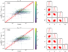 |
Fig. 3 L− T scaling relations and the posterior distributions of the scaling relations parameters. Left: soft band (0.5−2.0 keV) X-ray luminosity (Lx), bolometric (0.01–100 keV) luminosity (Lbol), temperature (T), and redshift (z) measurements of the ℒdet > 15, ℒext > 15 sample and the best-fit scaling relation models. The light red shaded area indicates the lσ uncertainty of the mean of the log-normal model (see Eq. (5)) and the dashed red line indicates the best-fit standard deviation (σL|T) around the mean. Orange diamonds indicate median temperature measurements obtained from clusters between luminosity quantiles. Right: parameter constraints of the Lx − T and Lbol − T relations obtained from the second half of the MCMC chains. Marginalized posterior distributions are shown on the diagonal plots and the joint posterior distributions are shown on off-diagonal plots. Red dashed vertical lines indicate the 32th, 50th, and 68th percentiles and contours indicate 68 and 95% credibility regions. |
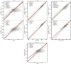 |
Fig. 4 Comparison between our best-fit L− T, L− Mgas, L − YX, and Mgas − T relations, the self-similar model and other studies in the literature (Maughan 2007; Arnaud et al. 2007; Zhang et al. 2008, 2011; Pratt et al. 2009; Eckmiller et al. 2011; Lovisari et al. 2015; Mantz et al. 2016). Grey circles are the eFEDS clusters. In order to achieve consistency, a cosmology and energy band conversion is applied to the previously reported results (see Sect. 4 for the details). |
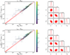 |
Fig. 5 L − Mgas scaling relations and the posterior distributions of the scaling relations parameters. Left: soft band (0.5−2.0 keV) X-ray luminosity (Lx)> bolometric (0.01–100 keV) luminosity (Lbol), gas mass (Mgas), and redshift (z) measurements of the ℒdet > 15, ℒext > 15 sample and the best-fit scaling relation models. The light-red shaded area indicates the 1σ uncertainty of the mean of the log-normal model (see Eq. (5)) and the dashed red line indicates the best-fit standard deviation |

4.2 Lx - Mgas snd Lbol − Mgas relations
Luminosity and gas mass are two tightly related observables because of their mutual dependence on electron density, and therefore a strong correlation is expected between them. Measurement of their correlation whilst taking into account selection effects and the mass function with a large sample allows us to test the theorized relation between these observables. According to the self-similar model, they are connected as
 (13)
(13)
and
 (14)
(14)
Our best-fit results for the Lx − Mgas and Lbol − Mgas relations are provided in Table 5 and in Fig. 5. A comparisons of these results with previous work is shown in Fig. 4. We report a slopeof  redshift evolution term of
  , and a scatter of
  . The slope is in tension with the self-similar expectation at a 5σ level, but the redshift evolution is consistent with the self-similar model within 2σ confidence for the LX − Mgas relation. When we fix the redshift evolution to the self-similar value, the slope does not change significantly (B = 1.07 ± 0.02). Zhang et al. (2011) obtained a slope of B = 1.11 ± 0.03 from the 62 clusters in the HIFLUGCS sample which is consistent with our measurements. Their slope for the cool-core clusters (B = 1.09 ± 0.05) is similar to what they found for their whole cluster sample, but the best-fit slope for their noncool-core clusters is steeper (B = 1.20 ± 0.06). Lovisari et al. (2015) studied the scaling properties of a complete X-ray-selected galaxy group sample and found the slope of the LX − Mgas relation for galaxy groups to be B = 1.02 ± 0.24, which is slightly shallower than but still consistent with the result they obtained for more massive clusters, B = 1.18 ± 0.07. Both of these measurements are consistent with our slope. On the other hand, a flux-limited sample of 139 clusters compiled from the ROSAT All-Sky Survey catalog has a steeper slope with B = 1.34 ± 0.05 for the Lx − Mgas relation (Mantz et al. 2016). The result of these latter authors is more than 4σ away from our measurement. This discrepancy might be due to the fact that the Mantz et al. (2016) sample is dominated by massive luminous clusters (their lowest luminosity system is about as bright as our most luminous systems), while the eFEDS sample is composed of low-mass clusters and groups. There are not many studies in the literature reporting intrinsic scatter of the LX − Mgas relation. Therefore, we were only able to compare our results with those of Zhang et al. (2011), who found
  , which is significantly lower (5.5σ) than our results.
On the other hand, we find the best-fit parameters of the slope, the evolution term, and the scatter of the Lbol − Mgas relation are  , and
, and  , respectively. Similarly, the slope is ~5σ away from the self-similar model, while the redshift evolution is fully consistent with the model. This relation has received much less attention in the literature. Zhang et al. (2011) found a slope of B = 1.29 ± 0.05 when they fitted their whole sample. Their reported slope is less steep for cool-core clusters (B = 1.24 ± 0.05) relative to the noncool-core clusters (B = 1.42 ± 0.06). The slope of the whole sample is fully consistent with our measurements within 2σ. Similar to the LX − Mgas relation, we could only compare our best-fit intrinsic scatter for the Lbol − Mgas relation with the results of Zhang et al. (2011), who report
  , which is in 4σ tension with our results.
One additional point is that there is a noticeable deviation around the gas mass of ~1012 M⊙ in Fig. 5. The low-mass groups tend to show higher luminosity relative to the mass determined from the scaling relations. The slope and normalization of this power-law relation are mostly governed by the higher mass clusters. The low-mass groups would prefer a shallower LX − Mgas power-law slope relative to the high-mass clusters. This observed trend is fully consistent with the LX − Mgas relation reported by Lovisari et al. (2015), who similarly observed the relation getting shallower at the group scale but within error bars.
4.3 LX − YX and Lbol − YX relations
The accurate mass indicator, YX, first introduced by Kravtsov et al. (2006), shows a low intrinsic scatter with mass and has a tight relation with the Sunyaev Zel’dovich (SZ) effect observable Compton-y parameter, YSZ (e.g., Maughan 2007; Benson et al. 2013; Mantz et al. 2016; Bulbul et al. 2019; Andrade-Santos et al. 2021). Because of this strong correlation, scaling relations involving YX can be used as a connection in multi-wavelength studies of galaxy clusters. Numerical simulations suggest that nongravitational effects have a small influence on this mass proxy compared to other X-ray observables (Nagai et al. 2007).
According to the self-similar model, luminosity is expected to depend on YX and redshift as
 (15)
(15)
and
 (16)
(16)
Our results for the best-fit LX − YX relations are listed in Table 5 and plotted in Fig. 6, while a comparison with the literature is provided in Fig. 4. We find a slope of B = 0.83 ± 0.02, a redshift evolution exponent of 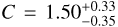 , and an intrinsic scatter of
  for the LX − YX scaling relation. Our slope for the LX − YX relation is 11.5σ steeper than that predicted by the self-similar model. The redshift evolution of the LX − YX relation is slightly shallower than the self-similar expectation but is consistent within the uncertainties. Our slope is consistent with the results presented in Maughan (2007) (B = 0.84 ± 0.03) and with that of Lovisari et al. (2015) (B = 0.79 ± 0.03). Our results for the same relation are within 1.8σ- statistical uncertainty of the HIFLUGCS+groups sample of Eckmiller et al. (2011) and within 2.2σ of their groups-only sample. These latter authors find slopes of B = 0.78 ± 0.02 and B = 0.71 ± 0.05 for the HIFLUGCS+groups and groups only samples, respectively, where the latter is within ~2σ from the self-similar expectation. Our best-fit intrinsic scatter is in good agreement (1.5σ) with the findings of Pratt et al. (2009)
  . Eckmiller et al. (2011)
  and Lovisari et al. (2015)
  report higher values for the intrinsic scatter of the LX − YX relation, but these measurements are presented without error bars and therefore a statistical comparison with our findings cannot be made.
For the Lbol − YX relation, we find a slope of B = 0.90 ± 0.02, a redshift evolution exponent of 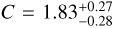 , and an intrinsic scatter of
  . The slope shows a 5σ deviation from self-similarity. Maughan (2007) find an even larger deviation from the self-similarity, measuring a slope of B = 1.10 ± 0.04. Also, in Zhang et al. (2008) and Pratt et al. (2009), the authors reported steeper slopes of B = 0.95 ± 0.08 and B = 1.04 ± 0.06 where the former agrees well with our results within statistical uncertainties whereas the latter is 2.2σ higher. Numerical simulations show a similar scenario. Biffi et al. (2014) reports this slope to be B = 0.94 ± 0.02, which is also slightly steeper than our results and significantly steeper than the self-similar value. Our redshift evolution for the Lbol − YX relation is consistent with the self-similar prediction within the uncertainties. A similar redshift evolution was measured in Maughan (2007), with C = 2.2 ± 0.1 which is <1.5σ away from our finding. Our best-fit intrinsic scatter for the Lbol − YX relation is slightly smaller (1.5σ) compared to the value reported in Pratt et al. (2009)
  . Maughan (2007) reported a similar value
  for the intrinsic scatter that is in 2.2σ tension with our best-fit value.
4.4 Mgas −T relation
Mgas − T and LX − T relations are conjugates of each other because of the tight correlation between Mgas and LX. However, we still expect to see differences as Mgas has a linear dependence on electron density whereas L has a quadratic dependence. We fit the Mgas − T relation following the similar framework as in the sections above with minor changes. We use the LX flavored selection function by converting Mgas to LX because we do not have a selection function involving Mgas from simulations. This one-to-one conversion in principle should not introduce a large bias to our results because Lx and Mgas are tightly correlated and the scatter between them is relatively low.
Based on the self-similar model, gas mass and temperature should be related to each other via
 (17)
(17)
Our results for the Mgas − T relation are listed in Table 5 and shown in Fig. 7. We obtain a slope of B = 2.41 ± 0.11, a redshift evolution exponent of  and a scatter of
  . Our slope is 8.3σ steeper than the self-similar model. We find a positive redshift evolution which is expected to be negative in the self-similar case, but our result agrees with the self-similar prediction within 1.5σ statistical uncertainty. A comparison of our results with the literature is given in Fig. 4. In general, the slope of the Mgas − T relation reported in the literature is close to ~1.9, which is steeper than the self-similar expectation. Reported slopes in the literature show a dependency on the mass range of the parent sample. For instance, Arnaud et al. (2007) reports a slope of 2.10 ± 0.05 based on the XMM-Newton observations of ten relaxed nearby clusters. Consistently, Croston et al. (2008) found 1.99 ± 0.11 using the 31 clusters in the REXCESS sample and Zhang et al. (2008) obtained 1.86 ± 0.19 with XMM-Newton data for 37 LoCuSS clusters. These slopes are shallower than the results reported here, with a 2.5σ difference. The discrepancy could be due to the different selection of the samples compared here.
We find a factor of approximately two difference when we compare our best-fit normalization results with those of Arnaud et al. (2007) and Croston et al. (2008) at their pivot temperature value (5 keV). To investigate this difference and test our results, we reconstructed the Mgas − T relation using our best-fit Lx − T and LX − Mgas relations, which are in agreement with the most recent studies in the literature taking into account the selection effects. We obtain a relation of
 (18)
(18)
The normalization, slope, and evolution terms are <2σ away from the best-fit Mgas − T relation which indicates that our results for the Mgas − T relation would be in good agreement with the previous results if the selection effects were taken into account. We argue that the observed discrepancy arises due to the combined effect of two main differences between our analyses and the other analyses reported in the literature for the same relation. The first difference is that we include selection effects in our work and therefore measure a steeper slope for the Mgas − T relation compared to the previously reported results. Our steeper slope agrees well with previous findings because Mgas is a very good Lx proxy and many studies, including ours, show that the best-fit slope of the LX−T relation is found to be steeper when the selection effects are taken into account. The second difference is that our sample includes a larger fraction of low-mass clusters compared to the other samples. If the cluster populations were similar, we would not observe such a difference in normalization even if the slopes did not match. Therefore, in our case, the populations and the slopes being different combine and result in the observed mismatch. Additionally, using a converted flavored selection function might have also contributed to the discrepancy, but its effect is expected to be much smaller because the relation between Lx and Mgas is tight and the scatter is low.
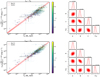 |
Fig. 6 L − Yx scaling relations and the posterior distributions of the scaling relations parameters. Left: soft band (0.5–2.0 keV) X-ray luminosity (Lx)> bolometric (0.01–100 keV) luminosity (Lbol), Yx, and redshift (z) measurements of the ℒdet > 15, ℒext > 15 sample and the best-fit scaling relation models. The light-red shaded area indicates the 1σ uncertainty of the mean of the log-normal model (see Eq. (5)) and the dashed red line indicates the best-fit standard deviation |

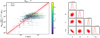 |
Fig. 7 Mgas − T scaling relation and the posterior distributions of the scaling relation parameters. Left: gas mass (Mgas), temperature (T), and redshift (z) measurements of the ℒdet > 15, ℒext > 15 sample and the best-fit scaling relation models. The light-red shaded area indicates the 1σ uncertainty of the mean of the log-normal model (see Eq. (5)) and the dashed red line indicates the best-fit standard deviation |

5 Discussion
Slopes of the scaling relations between X-ray observables studied in this work show deviations from the self-similar model by 4-11.5σ confidence levels. These deviations are often attributed to the departures from the assumptions in the self-similar (Kaiser 1986) model in the literature. We discuss two potential reasons for the observed discrepancy in the eFEDS sample in this section.
The most commonly proposed explanations in the literature for the departures from self-similarity challenge two major assumptions in the model. First, clusters are assumed to have a spherically symmetric gas distribution that is in hydrostatic equilibrium. Secondly, physical processes are majorly driven by the gravitational force, and the other effects are negligible in shaping the observed physical state of clusters. Observational data and numerical simulations indicate that both of these assumptions may not hold, and this can lead to departures from the self-similar expectation. Nongravitational processes such as AGN feedback, galactic winds, and star formation introduce extra energy to the system, heat the gas, and increase the entropy in the core (e.g., Voit 2005; Walker et al. 2012; Bulbul et al. 2016). AGN feedback in particular can play an important role in shaping the gas physics, especially in low-mass clusters and groups that dominate the eFEDS extended source sample. AGN activity can expel gas to the outskirts for lower mass haloes because of their shallower potentials wells. As the larger fraction of gas is removed from the centers of low-mass haloes, their luminosity decreases (e.g., Puchwein et al. 2008). The most massive clusters with deeper potential wells, higher total mass, and the ICM temperature are less affected by the nongravitational effects. When the clusters and groups are fit together, the lower luminosity of the groups and low-mass clusters leads to a steeper slope of the LX−T scaling relations when the cores are included. This result is consistent with numerical simulations (Puchwein et al. 2008; Schaye et al. 2010; Biffi et al. 2014; Truong et al. 2018; Henden et al. 2018, 2019), and the observational data in the literature (Eckmiller et al. 2011; Maughan et al. 2012; Pratt et al. 2009; Zou et al. 2016; Giles et al. 2016; Migkas et al. 2020; Lovisari et al. 2021). Another proposed reason for these steep slopes is the use of the overdensity radii R500 derived from the X-ray masses calculated assuming the hydrostatic equilibrium (see Lovisari et al. 2021, for discussion). If the radius R500 is biased low because of the unaccounted-for nonthermal pressure in the ICM, the luminosity extracted in this radius would be lower. The temperatures are less impacted by this effect, because of large uncertainties. However, in this work, we use the overdensity radii R500 obtained from the HSC weak lensing measurements uniformly for low-mass groups and clusters in the eFEDS sample (Chiu et al. 2022). We argue that the (mass-dependent) hydrostatic equilibrium bias and radius of extraction do not have a major effect in this work and cannot explain the steepening slope of the Lx − T scaling relations. The Mgas − T relations should be affected by the AGN feedback similarly but less severely than the Lx − T relation because of the linear dependence of Mgas on the number density of electrons, i.e., Mgas ∝ ne while  through X-ray emissivity. The expected steepening in Mgas − T should be less prominent as a result of this effect. This is fully consistent with our results assuming that the discrepancy is attributed to nongravitational effects. Another important issue in comparing various results in the literature is the calibration differences between X-ray telescopes. The number density and luminosity measurements are expected to be consistent between X-ray telescopes, namely Chandra and XMM-Newton (Bulbul et al. 2019); however, significant band-dependent disagreements have been reported for cluster ICM temperature measurements (Schellenberger et al. 2015). Given that the reported discrepancies between X-ray instruments are small in the soft X-ray band where the temperature measurements of most of our clusters lie, we do not expect that the slope differences are due to these calibration effects.
For Lx − YX and Lx − Mgas scaling relations, the effect of Malmquist bias, i.e., preferential sampling of bright objects, can clearly be seen and is often prominent in X-ray-selected samples. We note that these biases and selection effects are fully accounted for in our selection function, and therefore should not bias our best-fit scaling relations. We observe mild deviations from the self-similar model on both scaling relations in low Mqas and YX regimes. The mass proxy YX shows low intrinsic scatter with cluster mass in the literature (Kravtsov et al. 2006; Eckmiller et al. 20ll; Bulbul et al. 2019). As the ICM temperature scales with total mass, we expect to see a similar trend with low-scatter in the Lx − YX scaling relations. Indeed, the Lx − YX scaling relations show a tight correlation for massive clusters. Along the lines of what we observe, as the group scales dominate the sample, the intrinsic scatter becomes larger. We find that the departures from the self-similarity are significant for both of the relations which is consistent with the results reported in the literature and numerical simulations (Eckmiller et al. 20ll; Biffi et al. 2014; Lovisari et al. 2015).
The self-similar model predicts cosmology-dependent redshift evolution for the scaling relations between observables and cluster mass. This dependence is introduced through the overdensity radius (and the critical density), which is inversely related to the evolution of the Hubble parameter with redshift z, E(z) − H(z)/H0. We do not find significant departures from the self-similar evolution with redshift in any of our relations. All show self-similar redshift evolution <2.5σ confidence level. There are contradictory reports in the literature as to the evolution of scaling relations. Some studies report self-similar redshift evolution with redshift (Giodini et al. 2013), while some studies report no evolution (Maughan 2007; Pacaud et al. 2007). Larger samples, covering a wide redshift range, will be available with the eRASS data, which can be used to constrain the redshift evolution of scaling relations and test the self-similar model.
In this work, we investigate the scaling relations between X-ray observables of the clusters of galaxies and galaxy groups by fully modeling the selection effects. Our method of obtaining the selection function relies on realistic simulations of the eROSITA observations. This is the most robust way of modeling the selection effects as long as the simulated population of sources is representative of the observed sample. The advantage of this method lies in the fact that the same detection and reduction methods are applied to both simulated observations and the eROSITA data self-consistently (Clerc et al. 2018; Comparat et al. 2020). In these simulations, cluster surface brightness profiles are created by making use of the previously measured profiles of cluster and group samples that span a wide range of mass and redshift; they use X-COP, SPT, XXL, and HIFLUGCS cluster samples. This method allows the profiles to be consistent with the observations, except in the low-L, low-z regime where we probe a mass and redshift space that is poorly explored by previous X-ray observations. This led to a slight excess in the number of detected simulated clusters by the pipeline in this parameter space, the presence of which is barely visible in Fig. 2. The mild difference does not have any effect on our best fitting relations because our likelihood takes the redshift (z) and detection (I) information of clusters as given,  , such that in our analysis, the shape of P(I|Lx, z) as a function of Lx is more important than the relative normalizations at different redshifts, P(I|z) = ∫P(I|Lx, z)P(LX|z)dLX.
Following our analysis of the eFEDS observations, this less populated mass-luminosity range will be filled with eFEDS clusters, and therefore surface brightness profiles of simulated clusters at these regimes will be improved for modeling the selection function for the future eRASS observations. Proper modeling of the selection effects will be particularly important for placing constraints on cosmological parameters using eROSITA observations (Clerc et al. 2018).
We also test our method by comparing the model-predicted number of detected clusters (Ndet) and the number of clusters in our observed sample  as also presented in Giles et al. (2016). However, we find that comparing the predicted and observed cluster numbers is not informative because the predictions have large uncertainties driven mostly by the propagated errors from our scaling relation analysis and the weak-lensing mass-calibrated scaling relation analysis (Chiu et al. 2022). To give an example, we compare the observed number of detected clusters for the ℒdet > 15, ℒext > 15 sample (265) with the model-predicted number for the Lx − T relation similar to the Giles et al. (2016). We calculated Ndet as
 (19)
(19)
where is the differential comoving volume shell spanning a solid angle of
  is the temperature function calculated as described in Sect. 3.2, and
  is the best-fit parameters of the Lx − T relation. While calculating Ndet, first we only propagate the errors of the best-fit parameters <ieq/ using MCMC chains and a pivot value of Mpiv = 1.4 × 10¹⁴M⊙, which is the median of the eFEDS sample. We find the model-predicted number of detected clusters to be
  . When we further propagate both the uncertainties of
  and the best-fit weak-lensing mass-calibrated scaling relation parameters (AX, BX, yX), we find the new measurement to be
  . In this case, the observed number of clusters is consistent with the predicted number of clusters within the uncertainties. The difference in the absolute values might be due to the selection function, or the cosmology-dependent normalization of the mass function. In this work and simulations, we use the Planck cosmology (Planck Collaboration XIII 2016) with the Tinker et al. (2008) mass function. Larger samples of clusters of galaxies will soon be available through the eROSITA All-Sky observations and these will provide sufficient statistics to constrain the cosmology simultaneously with the scaling relations (see Pillepich et al. 2012, for the cosmology forecast).
Decreasing the scatter is of significant importance in reducing the systematic error on the constraints of cosmological parameters through cluster counts. Cool-core and relaxed clusters are reported to show less scatter on the scaling relations relative to the mergers (Vikhlinin et al. 2009; Mantz et al. 2010b). The dynamical states of the eFEDS clusters and groups were presented by Ghirardini et al. (2021). The dynamically relaxed clusters compose 30–40% of this sample, and therefore using them reduces the statistical power of our measurements. Additionally, the use of the relaxed cluster in the scaling-relation fits requires a selection function characterized in terms of these morphological parameters and a dynamical-state-dependent mass function (e.g., Seppi et al. 2021). This form of selection function is not available yet. We therefore leave this work to future studies of the eRASS data.
6 Conclusions
The eFEDS is of a similar depth to the final eROSITA All-Sky Survey in Equatorial regions. In this field, we detect 542 galaxy clusters and groups in the extent-selected sample with an addition of 347 clusters of galaxies in the point source samples (Liu et al. 2022a; Klein et al. 2022; Bulbul et al. 2022). In this work, we present the X-ray properties (Lx, Lbol, T, Mgas, YX) of the all eFEDS clusters and groups measured in two apertures; core-included (r < R500) and core-excluded (0.15 R500 < r < R500). The overdensity radius R500 is obtained from the HSC weak-lensing mass estimates provided by Chiu et al. (2022), allowing our measurements to be free of bias from the hydrostatic equilibrium assumption. This work clearly demonstrates that the cluster ICM emission will be significantly detected for most of the clusters in the mass and redshift ranges out to R500 at this depth.
Additionally, we provide the L − T, L − Mgas, L − YX, and Mgas − T scaling relations between these (core-included) X-ray observables for a subsample of clusters. We only consider the extent-selected sample, where we can characterize the selection effects using the state-of-the art simulations. Contamination of the main eFEDS clusters and groups sample by AGNs and false detections due to fluctuations is on the order of 20% (see Liu et al. 2022a,b, for details). To reduce the contamination of the sample to under 10%, we further apply the cuts on the extent and detection likelihoods of ℒdet > 15 and ℒext > 15. We note that, apart from the ℒdet and ℒext cuts, we have not applied any further cleaning to the sample, such as optical cross-matching. These cuts reduce the sample size to 265 clusters and groups spanning a redshift range of 0.017 < z < 0.94, a soft-band luminosity range of 8.64 × 1040 erg s−1 < Lx < 3.96 × 1044 erg s−1, and a mass range of 6.86 × 10¹² M⊙ < M500 < 7.79 × 10¹⁴ M⊙. In this sample, we find 68 low-mass galaxy groups with <1014 M⊙, which are uniformly selected with the rest of the massive clusters in the sample. We investigated these seven relations by taking into account both the selection effects and the cosmological distributions of observables. Fitting was performed twice for each of the seven relations, first with a redshift evolution exponent left free and the second with a redshift evolution exponent fixed to the corresponding self-similar value. The main conclusions of our analysis are as follows:
The eFEDS scaling-relation results between X-ray observables in general are in good agreement with the recently reported results. However, we find significant tension with the self-similar expectation for all scaling relations studied here. We suggest that these deviations indicate that the nongravitational effects such as the feedback mechanisms play a key, nonnegligible role in shaping the observed physical properties of the clusters, especially in the low-mass group regime. Specifically, the scaling-relation results we present in this paper for the L − T relation agree well with the results from the samples that are similar to the eFEDS sample when the selection function is taken into account (Giles et al. 2016; Lovisari et al. 2015; Eckmiller et al. 2011). Our results for the L − T relation also agree well with the fable and MACSIS simulations where they include baryonic feedback (Puchwein et al. 2008; Henden et al. 2019; Biffi et al. 2014; Barnes et al. 2017).
The largest scatter we measure is for the Lx − T and Lbol − T relations. We find
 when we fix the redshift evolution to the self-similar value and
  when the evolution is let free. This intrinsic scatter is mostly driven by the groups. The lowest scatter is measured for the Lx − YX and Lbol − YX relations with
  . This result shows that in addition to YX being a good mass indicator, it is also a good proxy for the X-ray properties of the ICM.
The redshift evolution of the scaling relations of the seven scaling relations we examined is broadly consistent with the self-similar model. Fixing the redshift evolution exponent to the corresponding self-similar value only changes the best-fit slopes by < 1σ from its previous value obtained with a free exponent. Larger samples of clusters and groups are required for constraining the evolution of these relations with redshift.
We find that the Mgas − T relation differs from the previous results in the literature by a factor of approximately two in normalization. This could be driven by the lack of proper consideration of the selection effects in the previously reported results or by the fact that the eFEDS sample contains a much greater number of low-mass clusters and groups than the compared samples. This difference might also partially be due to the lack of a selection function with the Mgas flavor. Inclusion of X-ray observables other than Lx and Lbol in the simulations is an ongoing project, and will help to understand the effects of such phenomena.
This work extends the study of X-ray scaling relations to a sample that is dominated by low-mass clusters and groups. It crates a further avenue by which to study ICM physics for a new population of low-mass clusters and groups, as well as massive clusters at a wide redshift range. These initial results demonstrate the capability of eROSITA to detect the ICM emission out to R500 for a large number of clusters detected at the final depth of the All Sky Survey. We note that this depth will be exceeded by the first All Sky Survey for a limited area, allowing the observables to be measured out to R500 or beyond for a subsample of clusters. These measurements will provide access to increasingly stringiest constraints on the mass and redshift evolution of the scaling relations. eFEDS observations not only allow us to put tight constraints on the scaling relation parameters but also allow us to test our selection function, which will be used in future statistical studies with eROSITA.
Acknowledgement.
This work is based on data from eROSITA, the soft X-ray instrument aboard SRG, a joint Russian-German science mission supported by the Russian Space Agency (Roskosmos), in the interests of the Russian Academy of Sciences represented by its Space Research Institute (IKI), and the Deutsches Zentrum für Luft und Raumfahrt (DLR). The SRG spacecraft was built by Lavochkin Association (NPOL) and its subcontractors, and is operated by NPOL with support from the Max Planck Institute for Extraterrestrial Physics (MPE). The development and construction of the eROSITA X-ray instrument was led by MPE, with contributions from the Dr. Karl Remeis Observatory Bamberg and ECAP (FAU Erlangen-Nuernberg), the University of Hamburg Observatory, the Leibniz Institute for Astrophysics Potsdam (AIP), and the Institute for Astronomy and Astrophysics of the University of Tubingen, with the support of DLR and the Max Planck Society. The Argelander Institute for Astronomy of the University of Bonn and the Ludwig Maximilians Universitat Munich also participated in the science preparation for eROSITA. The eROSITA data shown here were processed using the eSASS software system developed by the German eROSITA consortium. The Hyper Suprime-Cam (HSC) collaboration includes the astronomical communities of Japan and Taiwan, and Princeton University. The HSC instrumentation and software were developed by the National Astronomical Observatory of Japan (NAOJ), the Kavli Institute for the Physics and Mathematics of the Universe (Kavli IPMU), the University of Tokyo, the High Energy Accelerator Research Organization (KEK), the Academia Sinica Institute for Astronomy and Astrophysics in Taiwan (ASIAA), and Princeton University. Funding was contributed by the FIRST program from the Japanese Cabinet Office, the Ministry of Education, Culture, Sports, Science and Technology (MEXT), the Japan Society for the Promotion of Science (JSPS), Japan Science and Technology Agency (JST), the Toray Science Foundation, NAOJ, Kavli IPMU, KEK, ASIAA, and Princeton University. This paper makes use of software developed for the Large Synoptic Survey Telescope. We thank the LSST Project for making their code available as free software at http://dm.lsst.org. This paper is based (in part) on data collected at the Subaru Telescope and retrieved from the HSC data archive system, which is operated by the Subaru Telescope and Astronomy Data Center (ADC) at National Astronomical Observatory of Japan. Data analysis was in part carried out with the cooperation of Center for Computational Astrophysics (CfCA), National Astronomical Observatory of Japan. The Subaru Telescope is honored and grateful for the opportunity of observing the Universe from Maunakea, which has the cultural, historical and natural significance in Hawaii. E.B. acknowledges financial support from the European Research Council (ERC) Consolidator Grant under the European Union’s Horizon 2020 research and innovation programme (grant agreement No 101002585). N.C. is supported by CNES.
References
- Aihara, H., Arimoto, N., Armstrong, R., et al. 2018, PASJ, 70, S4 [NASA ADS] [Google Scholar]
- Andrade-Santos, F., Pratt, G. W., Melin, J.-B., et al. 2021, ApJ, 914, 58 [NASA ADS] [CrossRef] [Google Scholar]
- Arnaud, M., Pointecouteau, E., & Pratt, G. W. 2007, A&A, 474, L37 [CrossRef] [EDP Sciences] [Google Scholar]
- Ascasibar, Y., Sevilla, R., Yepes, G., Müller, V., & Gottlöber, S. 2006, MNRAS, 371, 193 [NASA ADS] [CrossRef] [Google Scholar]
- Asplund, M., Grevesse, N., Sauval, A. J., & Scott, P. 2009, ARA&A, 47, 481 [NASA ADS] [CrossRef] [Google Scholar]
- Babul, A., Balogh, M. L., Lewis, G. F., & Poole, G. B. 2002, MNRAS, 330, 329 [NASA ADS] [CrossRef] [Google Scholar]
- Barnes, D. J., Kay, S. T., Henson, M. A., et al. 2017, MNRAS, 465, 213 [Google Scholar]
- Benson, B. A., de Haan, T., Dudley, J. P., et al. 2013, ApJ, 763, 147 [NASA ADS] [CrossRef] [Google Scholar]
- Bhattacharya, S., Di Matteo, T., & Kosowsky, A. 2008, MNRAS, 389, 34 [NASA ADS] [CrossRef] [Google Scholar]
- Biffi, V., Sembolini, F., De Petris, M., et al. 2014, MNRAS, 439, 588 [NASA ADS] [CrossRef] [Google Scholar]
- Blanton, M. R., Bershady, M. A., Abolfathi, B., et al. 2017, AJ, 154, 28 [Google Scholar]
- Bocquet, S., Dietrich, J. P., Schrabback, T., et al. 2019, ApJ, 878, 55 [Google Scholar]
- Borgani, S., Governato, F., Wadsley, J., et al. 2002, MNRAS, 336, 409 [NASA ADS] [CrossRef] [Google Scholar]
- Brunner, H., Liu, T., Lamer, G., et al. 2022, A&A, 661, A1 (eROSITA EDR SI) [NASA ADS] [CrossRef] [EDP Sciences] [Google Scholar]
- Bulbul, G. E., Hasler, N., Bonamente, M., & Joy, M. 2010, ApJ, 720, 1038 [NASA ADS] [CrossRef] [Google Scholar]
- Bulbul, E., Randall, S. W., Bayliss, M., et al. 2016, ApJ, 818, 131 [Google Scholar]
- Bulbul, E., Chiu, I. N., Mohr, J. J., et al. 2019, ApJ, 871, 50 [Google Scholar]
- Bulbul, E., Liu, A., Pasini, T., et al. 2022, A&A, 661, A10 (eROSITA EDR SI) [NASA ADS] [CrossRef] [EDP Sciences] [Google Scholar]
- Capelo, P.R., Coppi, P.S., & Natarajan, P. 2012, MNRAS, 422, 686 [NASA ADS] [CrossRef] [Google Scholar]
- Chiu, I.-N., Ghirardini, V., Liu, A., et al. 2022, A&A, 661, A11 (eROSITA EDR SI) [NASA ADS] [CrossRef] [EDP Sciences] [Google Scholar]
- Clerc, N., Ramos-Ceja, M. E., Ridl, J., et al. 2018, A&A, 617, A92 [NASA ADS] [CrossRef] [EDP Sciences] [Google Scholar]
- Comparat, J., Merloni, A., Salvato, M., et al. 2019, MNRAS, 487, 2005 [Google Scholar]
- Comparat, J., Eckert, D., Finoguenov, A., et al. 2020, Open J. Astrophys., 3, 13 [Google Scholar]
- Croston, J. H., Pratt, G. W., Böhringer, H., et al. 2008, A&A, 487, 431 [NASA ADS] [CrossRef] [EDP Sciences] [Google Scholar]
- Dauser, T., Falkner, S., Lorenz, M., et al. 2019, A&A, 630, A66 [NASA ADS] [CrossRef] [EDP Sciences] [Google Scholar]
- Dey, A., Schlegel, D. J., Lang, D., et al. 2019, AJ, 157, 168 [Google Scholar]
- Driver, S.P., Norberg, P., Baldry, I.K., et al. 2009, Astron. Geophys., 50, 5.12 [NASA ADS] [CrossRef] [Google Scholar]
- Ebeling, H., Edge, A. C., Bohringer, H., et al. 1998, MNRAS, 301, 881 [Google Scholar]
- Eckmiller, H. J., Hudson, D. S., & Reiprich, T. H. 2011, A&A, 535, A105 [NASA ADS] [CrossRef] [EDP Sciences] [Google Scholar]
- Fabjan, D., Borgani, S., Tornatore, L., et al. 2010, MNRAS, 401, 1670 [Google Scholar]
- Finoguenov, A., Tanaka, M., Cooper, M., et al. 2015, A&A, 576, A130 [NASA ADS] [CrossRef] [EDP Sciences] [Google Scholar]
- Foreman-Mackey, D., Hogg, D. W., Lang, D., & Goodman, J. 2013, PASP, 125, 306 [Google Scholar]
- Foster, A. R., Ji, L., Smith, R. K., & Brickhouse, N. S. 2012, ApJ, 756, 128 [Google Scholar]
- Freyberg, M., Perinati, E., Pacaud, F., et al. 2020, SPIE Conf. Ser., 11444, 1144410 [Google Scholar]
- Ghirardini, V., Bulbul, E., Hoang, D. N., et al. 2021, A&A, 647, A4 [EDP Sciences] [Google Scholar]
- Ghirardini, V., Emre Bahar, Y., Bulbul, E., et al. 2022, A&A, 661, A12 (eROSITA EDR SI) [NASA ADS] [CrossRef] [EDP Sciences] [Google Scholar]
- Giles, P.A., Maughan, B.J., Pacaud, F., et al. 2016, A&A, 592, A3 [NASA ADS] [CrossRef] [EDP Sciences] [Google Scholar]
- Giodini, S., Lovisari, L., Pointecouteau, E., et al. 2013, Space Sci. Rev., 177, 247 [Google Scholar]
- Henden, N. A., Puchwein, E., Shen, S., & Sijacki, D. 2018, MNRAS, 479, 5385 [CrossRef] [Google Scholar]
- Henden, N. A., Puchwein, E., & Sijacki, D. 2019, MNRAS, 489, 2439 [NASA ADS] [CrossRef] [Google Scholar]
- Hilton, M., Romer, A. K., Kay, S. T., et al. 2012, MNRAS, 424, 2086 [NASA ADS] [CrossRef] [Google Scholar]
- Hogg, D. W. 1999, ArXiv e-prints [arXiv:astro-ph/9905116] [Google Scholar]
- Huchra, J. P., Macri, L. M., Masters, K. L., et al. 2012, ApJS, 199, 26 [Google Scholar]
- Iljenkarevic, J., Reiprich, T. H., Pacaud, F., et al. 2022, A&A, 661, A26 (eROSITA EDR SI) [NASA ADS] [CrossRef] [EDP Sciences] [Google Scholar]
- Kaiser, N. 1986, MNRAS, 222, 323 [Google Scholar]
- Kettula, K., Giodini, S., van Uitert, E., et al. 2015, MNRAS, 451, 1460 [CrossRef] [Google Scholar]
- Klein, M., Oguri, M., Mohr, J. J., et al. 2022, A&A, 661, A4 (eROSITA EDR SI) [NASA ADS] [CrossRef] [EDP Sciences] [Google Scholar]
- Kravtsov, A. V., & Borgani, S. 2012, ARA&A, 50, 353 [Google Scholar]
- Kravtsov, A. V., Vikhlinin, A., & Nagai, D. 2006, ApJ, 650, 128 [Google Scholar]
- Liu, A., Bulbul, E., Ghirardini, V., et al. 2022a, A&A, 661, A2 (eROSITA EDR SI) [NASA ADS] [CrossRef] [EDP Sciences] [Google Scholar]
- Liu, T., Merloni, A., Comparat, J., et al. 2022b, A&A, 661, A27 (eROSITA EDR SI) [NASA ADS] [CrossRef] [EDP Sciences] [Google Scholar]
- Lovisari, L., Reiprich, T. H., & Schellenberger, G. 2015, A&A, 573, A118 [NASA ADS] [CrossRef] [EDP Sciences] [Google Scholar]
- Lovisari, L., Schellenberger, G., Sereno, M., et al. 2020, ApJ, 892, 102 [Google Scholar]
- Lovisari, L., Ettori, S., Gaspari, M., & Giles, P. A. 2021, Universe, 7, 139 [NASA ADS] [CrossRef] [Google Scholar]
- Mantz, A. B. 2019, MNRAS, 485, 4863 [NASA ADS] [CrossRef] [Google Scholar]
- Mantz, A., Allen, S. W., Ebeling, H., Rapetti, D., & Drlica-Wagner, A. 2010a, MNRAS, 406, 1773 [NASA ADS] [Google Scholar]
- Mantz, A., Allen, S. W., Rapetti, D., & Ebeling, H. 2010b, MNRAS, 406, 1759 [NASA ADS] [Google Scholar]
- Mantz, A. B., von der Linden, A., Allen, S.W., et al. 2015, MNRAS, 446, 2205 [NASA ADS] [CrossRef] [Google Scholar]
- Mantz, A. B., Allen, S. W., Morris, R. G., et al. 2016, MNRAS, 463, 3582 [NASA ADS] [CrossRef] [Google Scholar]
- Maughan, B. J. 2007, ApJ, 668, 772 [Google Scholar]
- Maughan, B. J., Giles, P. A., Randall, S. W., Jones, C., & Forman, W. R. 2012, MNRAS, 421, 1583 [Google Scholar]
- McCarthy, I. G., Schaye, J., Ponman, T. J., et al. 2010, MNRAS, 406, 822 [NASA ADS] [Google Scholar]
- Merloni, A., Predehl, P., Becker, W., et al. 2012, ArXiv e-prints [arXiv:1209.3114] [Google Scholar]
- Migkas, K., Schellenberger, G., Reiprich, T. H., et al. 2020, A&A, 636, A15 [NASA ADS] [CrossRef] [EDP Sciences] [Google Scholar]
- Molham, M., Clerc, N., Takey, A., et al. 2020, MNRAS, 494, 161 [NASA ADS] [CrossRef] [Google Scholar]
- Nagai, D., Kravtsov, A. V., & Vikhlinin, A. 2007, ApJ, 668, 1 [Google Scholar]
- Pacaud, F., Pierre, M., Adami, C., et al. 2007, MNRAS, 382, 1289 [Google Scholar]
- Pacaud, F., Pierre, M., Melin, J. B., et al. 2018, A&A, 620, A10 [NASA ADS] [CrossRef] [EDP Sciences] [Google Scholar]
- Pierre, M., Pacaud, F., Juin, J. B., et al. 2011, MNRAS, 414, 1732 [Google Scholar]
- Pillepich, A., Porciani, C., & Reiprich, T. H. 2012, MNRAS, 422, 44 [Google Scholar]
- Planck Collaboration XIII. 2016, A&A, 594, A13 [NASA ADS] [CrossRef] [EDP Sciences] [Google Scholar]
- Pratt, G. W., Croston, J. H., Arnaud, M., & Böhringer, H. 2009, A&A, 498, 361 [NASA ADS] [CrossRef] [EDP Sciences] [Google Scholar]
- Pratt, G. W., Arnaud, M., Biviano, A., et al. 2019, Space Sci. Rev., 215, 25 [Google Scholar]
- Predehl, P., Andritschke, R., Arefiev, V., et al. 2021, A&A, 647, A1 [EDP Sciences] [Google Scholar]
- Puchwein, E., Sijacki, D., & Springel, V. 2008, ApJ, 687, L53 [NASA ADS] [CrossRef] [Google Scholar]
- Romer, A. K., Viana, P.T.P., Liddle, A.R., & Mann, R.G. 2001, ApJ, 547, 594 [NASA ADS] [CrossRef] [Google Scholar]
- Sanders, J. S., Biffi, V., Brüggen, M., et al. 2022, A&A, 661, A36 (eROSITA EDR SI) [NASA ADS] [CrossRef] [EDP Sciences] [Google Scholar]
- Schaye, J., Dalla Vecchia, C., Booth, C. M., et al. 2010, MNRAS, 402, 1536 [Google Scholar]
- Schellenberger, G., & Reiprich, T. H. 2017, MNRAS, 469, 3738 [CrossRef] [Google Scholar]
- Schellenberger, G., Reiprich, T. H., Lovisari, L., Nevalainen, J., & David, L. 2015, A&A, 575, A30 [NASA ADS] [CrossRef] [EDP Sciences] [Google Scholar]
- Seppi, R., Comparat, J., Nandra, K., et al. 2021, A&A, 652, A155 [NASA ADS] [CrossRef] [EDP Sciences] [Google Scholar]
- Short, C. J., Thomas, P.A., Young, O.E., et al. 2010, MNRAS, 408, 2213 [NASA ADS] [CrossRef] [Google Scholar]
- Smith, R. K., Brickhouse, N. S., Liedahl, D. A., & Raymond, J. C. 2001, ApJ, 556, L91 [Google Scholar]
- Tinker, J., Kravtsov, A. V., Klypin, A., et al. 2008, ApJ, 688, 709 [Google Scholar]
- Tozzi, P., & Norman, C. 2001, ApJ, 546, 63 [NASA ADS] [CrossRef] [Google Scholar]
- Truong, N., Rasia, E., Mazzotta, P., et al. 2018, MNRAS, 474, 4089 [NASA ADS] [CrossRef] [Google Scholar]
- Turner, D. J., Giles, P. A., Romer, A. K., et al. 2021, MNRAS, submitted [arXiv:2109.11807] [Google Scholar]
- Veronica, A., Su, Y., Biffi, V., et al. 2022, A&A, 661, A46 (eROSITA EDR SI) [NASA ADS] [CrossRef] [EDP Sciences] [Google Scholar]
- Vikhlinin, A., Kravtsov, A., Forman, W., et al. 2006, ApJ, 640, 691 [Google Scholar]
- Vikhlinin, A., Burenin, R. A., Ebeling, H., et al. 2009, ApJ, 692, 1033 [Google Scholar]
- Voit, G. M. 2005, Rev. Mod. Phys., 77, 207 [Google Scholar]
- Walker, S. A., Fabian, A. C., Sanders, J. S., & George, M. R. 2012, MNRAS, 427, L45 [Google Scholar]
- Whelan, B., Reiprich, T. H., Pacaud, F., et al. 2021, A&A, submitted [arXiv:2106.14545] [Google Scholar]
- Willingale, R., Starling, R. L. C., Beardmore, A. P., Tanvir, N. R., & O’Brien, P.T. 2013, MNRAS, 431, 394 [NASA ADS] [CrossRef] [Google Scholar]
- Wilms, J., Allen, A., & McCray, R. 2000, ApJ, 542, 914 [Google Scholar]
- Zhang, Y. Y., Finoguenov, A., Böhringer, H., et al. 2008, A&A, 482, 451 [NASA ADS] [CrossRef] [EDP Sciences] [Google Scholar]
- Zhang, Y. Y., Andernach, H., Caretta, C. A., et al. 2011, A&A, 526, A105 [NASA ADS] [CrossRef] [EDP Sciences] [Google Scholar]
- Zou, S., Maughan, B. J., Giles, P. A., et al. 2016, MNRAS, 463, 820 [Google Scholar]
R500 is the overdensity radius within which the density of the cluster is 500 times the critical density of the Universe at the cluster's redshift.
All Tables
X-ray observables of eFEDS clusters measured within R500 and between 0.15R500 − R500.
All Figures
|
Fig. 1 Left: redshift histogram of the ℒdet > 15, ℒext > 15 sample used in this work. Right: weak lensing calibrated total mass |
| In the text | |
|
Fig. 2 Soft band (0.5–2.0 keV) X-ray luminosity and redshift measurements of the clusters in the eFEDS field that satisfies the ℒdet > 15 and ℒext > 15 condition. Luminosities are measured within apertures of R500- White solid curves are smoothed contours of the Lx − z data points and the color is proportional to the PDF of the hypothetical Lx − z distribution modeled as P(I,Lx,z) = P(I|Lx,z)P(Lx|z)P(z) (see Sect. 3.3 for the description of the model). |
| In the text | |
|
Fig. 3 L− T scaling relations and the posterior distributions of the scaling relations parameters. Left: soft band (0.5−2.0 keV) X-ray luminosity (Lx), bolometric (0.01–100 keV) luminosity (Lbol), temperature (T), and redshift (z) measurements of the ℒdet > 15, ℒext > 15 sample and the best-fit scaling relation models. The light red shaded area indicates the lσ uncertainty of the mean of the log-normal model (see Eq. (5)) and the dashed red line indicates the best-fit standard deviation (σL|T) around the mean. Orange diamonds indicate median temperature measurements obtained from clusters between luminosity quantiles. Right: parameter constraints of the Lx − T and Lbol − T relations obtained from the second half of the MCMC chains. Marginalized posterior distributions are shown on the diagonal plots and the joint posterior distributions are shown on off-diagonal plots. Red dashed vertical lines indicate the 32th, 50th, and 68th percentiles and contours indicate 68 and 95% credibility regions. |
| In the text | |
|
Fig. 4 Comparison between our best-fit L− T, L− Mgas, L − YX, and Mgas − T relations, the self-similar model and other studies in the literature (Maughan 2007; Arnaud et al. 2007; Zhang et al. 2008, 2011; Pratt et al. 2009; Eckmiller et al. 2011; Lovisari et al. 2015; Mantz et al. 2016). Grey circles are the eFEDS clusters. In order to achieve consistency, a cosmology and energy band conversion is applied to the previously reported results (see Sect. 4 for the details). |
| In the text | |
|
Fig. 5 L − Mgas scaling relations and the posterior distributions of the scaling relations parameters. Left: soft band (0.5−2.0 keV) X-ray luminosity (Lx)> bolometric (0.01–100 keV) luminosity (Lbol), gas mass (Mgas), and redshift (z) measurements of the ℒdet > 15, ℒext > 15 sample and the best-fit scaling relation models. The light-red shaded area indicates the 1σ uncertainty of the mean of the log-normal model (see Eq. (5)) and the dashed red line indicates the best-fit standard deviation |
| In the text | |
|
Fig. 6 L − Yx scaling relations and the posterior distributions of the scaling relations parameters. Left: soft band (0.5–2.0 keV) X-ray luminosity (Lx)> bolometric (0.01–100 keV) luminosity (Lbol), Yx, and redshift (z) measurements of the ℒdet > 15, ℒext > 15 sample and the best-fit scaling relation models. The light-red shaded area indicates the 1σ uncertainty of the mean of the log-normal model (see Eq. (5)) and the dashed red line indicates the best-fit standard deviation |
| In the text | |
|
Fig. 7 Mgas − T scaling relation and the posterior distributions of the scaling relation parameters. Left: gas mass (Mgas), temperature (T), and redshift (z) measurements of the ℒdet > 15, ℒext > 15 sample and the best-fit scaling relation models. The light-red shaded area indicates the 1σ uncertainty of the mean of the log-normal model (see Eq. (5)) and the dashed red line indicates the best-fit standard deviation |
| In the text | |
Current usage metrics show cumulative count of Article Views (full-text article views including HTML views, PDF and ePub downloads, according to the available data) and Abstracts Views on Vision4Press platform.
Data correspond to usage on the plateform after 2015. The current usage metrics is available 48-96 hours after online publication and is updated daily on week days.
Initial download of the metrics may take a while.