| Issue |
A&A
Volume 661, May 2022
The Early Data Release of eROSITA and Mikhail Pavlinsky ART-XC on the SRG mission
|
|
|---|---|---|
| Article Number | A6 | |
| Number of page(s) | 13 | |
| Section | Catalogs and data | |
| DOI | https://doi.org/10.1051/0004-6361/202141133 | |
| Published online | 18 May 2022 | |
The eROSITA Final Equatorial-Depth Survey (eFEDS)
The Stellar Counterparts of eROSITA sources identified by machine learning and Bayesian algorithms
1
Hamburger Sternwarte
Gojenbergsweg 112
21029
Hamburg, Germany
e-mail: astro@pcschneider.eu
2
Max-Planck-Institut für extraterrestrische Physik
Giessenbachstrasse 1
85748
Garching, Germany
Received:
19
April
2021
Accepted:
16
June
2021
Stars are ubiquitous X-ray emitters and will be a substantial fraction of the X-ray sources detected in the on-going all-sky survey performed by the eROSITA instrument aboard the Spectrum Roentgen Gamma (SRG) observatory. We use the X-ray sources in the eROSITA Final Equatorial-Depth Survey (eFEDS) field observed during the SRG performance verification phase to investigate different strategies to identify the stars among other source categories. We focus here on Support Vector Machine (SVM) and Bayesian approaches, and our approaches are based on a cross-match with the Gaia catalog, which will eventually contain counterparts to virtually all stellar eROSITA sources. We estimate that 2060 stars are among the eFEDS sources based on the geometric match distance distribution, and we identify the 2060 most likely stellar sources with the SVM and Bayesian methods, the latter being named HamStars in the eROSITA context. Both methods reach completeness and reliability percentages of almost 90%, and the agreement between both methods is, incidentally, also about 90%. Knowing the true number of stellar sources allowed us to derive association probabilities pij for the SVM method similar to the Bayesian method so that one can construct samples with defined completeness and reliability properties using appropriate cuts in pij. The thus identified stellar sources show the typical characteristics known for magnetically active stars, specifically, they are generally compatible with the saturation level, show a large spread in activity for stars of spectral F to G, and have comparatively high fractional X-ray luminosities for later spectral types.
Key words: stars: activity / stars: coronae / X-rays: stars
© ESO 2022
1 Introduction
Stars with convective envelopes, that is, with stellar masses between 0.08 and 1.85 M⊙ (spectral types M to mid A) show magnetic activity and possess a corona emitting soft X-rays (λ ~ 1−100 Å). Stars of the same mass, however, can have very different X-ray properties, primarily depending on the stellar rotation period. The largest ratios between X-ray (LX) and bolometric luminosities (Lbol) are observed for rapidly rotating young stars, which show LX/Lbol ratios close to the so-called saturation limit of log LX/Lbol ~ −3 (Vilhu 1984; Pizzolato et al. 2003). On the other hand, old slowly rotating stars may have log LX/Lbol ~ −8 (see reviews by Güdel 2004; Testa et al. 2015). Since stars spin down with age, the stellar X-ray luminosity also declines with age (Skumanich 1972). Therefore, X-ray surveys are most sensitive to young stars and contain comparatively few old stars, hence, the parameter space of stellar activity is very unevenly sampled.
In addition to this inherent bias toward active stars, existing stellar samples with well characterized X-ray properties are relatively small, typically ≲1000 objects (Schmitt & Liefke 2004; Wright et al. 2011; Freund et al. 2018), compared to other stellar samples with hundreds of thousands of stars such as RAVE (Steinmetz et al. 2006), the Gaia-ESO survey (Gilmore et al. 2012), or even billions of stars (Gaia Collaboration 2016). The eROSITA all-sky survey, described in Predehl et al. (2021) and designated as eRASS:8, is expected to provide detections of almost 106 stars (see Merloni et al. 2012), thus bringing the sample count of X-ray emitting stars on par with other samples.
To harvest the full potential for stellar science, one needs to identify the stars among the other X-ray emitting objects in the eROSITA source list, that is, a classification task. The final data of the eROSITA all-sky survey will not be available before 2024, however, the eROSITA Final Equatorial Depth Survey (eFEDS) already provides the X-ray sensitivity expected after the completion of the all-sky survey for a field of ~140 square degrees (Brunner et al. 2022; Salvato et al. 2022). Hence, eFEDS provides an excellent opportunity to start the development of the methods required for the identification task.
The classification of large numbers of objects into different categories based on their measured properties is an old task and has been approached by different mathematical methods such as frequentist (e.g., Fischer 1938) or Bayesian procedures (Binder 1978). Nowadays, machine learning (ML) approaches are also popular thanks to improving algorithms, increasing computing power, and large datasets. These techniques are now regularly applied in the astrophysical context (e.g., Marton et al. 2019; Vioque et al. 2020, and Melton 2020 used ML techniques to identify young stars). Here, we present a Support Vector Machine (SVM) and a Bayesian method to identify stellar X-ray sources within the eROSITA source catalog.
The paper is structured as follows. We translate the task of identifying the stars into a classification problem in Sect. 2, present the SVM and Bayesian approaches in Sects. 3 and 4, compare their results in Sect. 5, and provide our conclusions as well as the outlook in Sect. 6.
2 The identification task
To identify and characterize the stellar eROSITA sources, we need information from other wavelengths in addition to the X-ray data. Specifically, the identification of the stellar content in eROSITA is based on matching the eROSITA sources to a catalog containing only eligible stellar counterparts, i.e., stars that may emit X-rays at flux levels detectable by eROSITA. An eROSITA source i is classified as stellar if an association between eROSITA source i and a counterpart j exists that has properties compatible with the hypothesis that counterpart j is responsible for the X-ray emission, that is, if one or more reasonable stellar counterparts (j1,…, jn) exist so that the association i ↔ j1 (or i ↔ j2, etc.) is likely while taking the possibility of chance alignments into account, too.
This approach differs from many other catalog cross-matching approaches in the sense that a complete identification of the eROSITA detections is not required: stars and non-stars are the only two relevant source categories for us, and only for objects in the first category do we attempt to find the correct counterpart (the problem of the identification, characterization and classification of the full eFEDS sample is discussed in Salvato et al. 2022). The non-stars category includes other source categories, mainly AGN (Liu et al. 2022) and nearby galaxies (Vulic et al. 2022), but also spurious X-ray detections, for example, due to background fluctuations. Objects in the nonstellar category are here treated as random associations and considered in a statistical sense. In summary, the categorization of the eROSITA sources is deferred to classifying the associations i ↔ j between eROSITA sources (i) and eligible stellar counterparts (j) as probable with respect to the alternative that the association is spurious, i.e., that object j in the match catalog is not responsible for X-ray source i.
In this scheme, the match catalog containing the eligible stellar counterparts is crucially important for the classification and must include counterparts to virtually all stellar eROSITA sources but may lack any other source category. The saturation limit for stars of log LX/Lbol ≈ −3 (Pizzolato et al. 2003; Wright et al. 2011) implies a limiting optical magnitude for reasonable stellar counterparts at any given X-ray sensitivity (the nominal LX/Lbol-values of some individual stars may exceed log LX/Lbol ≈ −3 in larger samples, but excursions toward significantly higher values are very rare). Figure 1 shows the Gaia magnitude that a star emitting X-rays at the saturation limit will have for the sensitivity of eFEDS, which is also approximately the limit for the eROSITA survey after eight passes (eRASS:8, see Predehl et al. 2021). In particular, virtually all stellar counterparts of eROSITA sources (eFEDS and eRASS) are expected to have G-magnitudes brighter than the detection limit of Gaia and, thus, will be eventually included in the Gaia catalog (Gaia Collaboration 2016). The Gaia catalog has the additional benefit of being all-sky and future data releases will improve the completeness to levels sufficient for identifying stars in the full eRASS survey; the current data release (EDR3) is already essentially complete for stars between G = 12 mag and 17 mag (Gaia Collaboration 2021). Given these beneficial properties, we chose to use the Gaia catalog as our match catalog (and magnitudes are therefore in the VEGAMAG system).
Our identification scheme aims to identify coronal emitters in quiescence. Stars occasionally flare, which can elevate the LX/Lbol quite significantly (see Boiler et al. 2022, for examples). Currently, stars undergoing flares during the eROSITA observations may show, depending on the specific star and flare, LX/Lbol-values that are so high (LX/Lbo1 ≫ −3) that they are deemed incompatible with stars in our schemes and, thus, may be misclassified as non-stellar (associations with LX/Lbol-values somewhat above −3 are typically still classified as stellar, see Fig. 6). The methods discussed here do not attempt to correct for the effects of flaring, because the observing sequence of the eROSITA all-sky survey differs from that of eFEDS. For eRASS, flares will be easily detected in the survey as each object is scanned multiple times.
We also note that we concentrate on coronal X-ray sources and that other galactic X-ray sources exist, which include genuine stars (e.g., cataclysmic variables). The origin of the X-ray emission in these objects, however, differs from the coronal emission seen in “normal” stars and they typically have high fractional X-ray luminosities. Therefore, they are also unlikely to be classified as stellar with our methods.
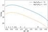 |
Fig. 1 Limiting G magnitude for stars emitting at X-ray activity levels of log LX/Lbol = −2.5 and −3 assuming the average eFEDS exposure depth. |
2.1 Input catalogs and data screening
The eROSITA and Gaia catalogs contain entries that are very unlikely to describe stars detected by eROSITA and we applied a number of filter criteria before performing the stellar identification to remove such catalog entries.
2.1.1 Stellar candidates in the eROSITA eFEDS catalog
We used eROSITA detections from the main eFEDS catalog, which contains sources detected in the energy range between 0.2 and 2.3 keV (see Brunner et al. 2022) and applied the following filter.
- 1.
No significant spatial extension (EXT_LIKE < 6), Extended sources are unlikely to represent stars unless they are a blend between two (or more) sources (expected to be very rare).
- 2.
Positive RADEC_ERR. There is a small number of eROSITA sources for which the source detection algorithm failed to calculate reasonable positional uncertainties. Because the positional uncertainty is a key value for our matching algorithms, we ignored sources with negative or zero RADEC_ERR entries.
Applying these criteria resulted in ΝX = 27 369 eROSITA detections, which constitute the X-ray input catalog abbreviated with χ in the following.
2.1.2 Eligible Gaia Counterparts
For the Gaia sources, we propagated coordinates from the Gaia EDR3 reference epoch (2016.0) to the epoch of the eFEDS observation (2019.85). Among the Gaia catalog entries, we selected those sources fulfilling the following conditions to be considered eligible counterparts to eROSITA detected stars.
- 1.
Gaia sources above the brightness limit given by the X-ray sensitivity, The eROSITA X-ray sensitivity limit combined with the range of LX/Lbol-ratios of stars (see Sect. 1) implies that eligible counter parts to eROSITA detections must have G ≲ 19 mag (for spectral types A to M, see Fig. 1).
- 2.
Gaia sources must have a three sigma significant parallax measurement (parallax_over_error > 3),
Gaia entries that do not have a significant parallax measurement are mostly extra galactic or galactic objects so distant (d ≫ 1 kpc) that they unlikely represent eligible counter parts to eROSITA detected stars.
- 3.
Gaia sources that fall into a rather generously defined region of the Gaia color-magnitude diagram (see Appendix A). This region includes young (1 Myr) and old (10 Gyr) stars with some margin to account for measurement errors. Regions in color-magnitude space where other objects such as cataclysmic variables (CVs) may be found are excluded (below the main sequence). We consider the stellar properties for objects outside this region to be too poorly known for our further analysis.
We did not filter the Gaia sources for RUWE, because we found that the sources with larger RUWE values1 have perfectly acceptable properties and suspect that the selection bias towards active stars and binaries or multiples may, at least partially, influence the astrometric solution leading to less than perfect RUWE values. In total, NG ≈ 4 × 10⁵ Gaia EDR3 counterparts fulfill our quality criteria (called ℊ in the following).
2.2 The catalog fraction
Among the properties describing any given eROSITA to Gaia association i ↔ j, the match distance is special: Measuring the sky positions with very high precision unambiguously informs us about the correct counterpart, and if such a counterpart does exist in the match catalog, because sources with too large match distances have negligible likelihoods to be the correct counterpart independent of all other parameters provided that source confusion is negligible.
This peculiarity of the sky positions provides a particularly beneficial information for the matching procedure, namely an estimate for the number of real matches, i.e., the fraction of eROSITA sources with a counterpart in the match catalog (the screened Gaia catalog), which we call the geometric catalog fraction (CF) in the following. The CF can be derived from the measured on-sky distances between the eROSITA sources and their nearest Gaia match, because the probability distributions to measure a particular match distance is known a priori for real and random associations. The distribution in match distance depends only on the positional uncertainty of the eROSITA source σi for real associations (in our context, Gaia sources have negligible positional uncertainties) and on the local sky density of eligible sources in the match catalog for random associations, respectively. Both properties can be measured independently of the nature of the eROSITA sources and its membership in the match catalog.
The CF is a sample property affecting all associations equally; it cannot be used to select any particular association over another association. For example, a CF of 0% would imply that even near perfect positional matches cannot be considered real while for a CF of 100%, large match distances are perfectly acceptable, because the correct counterpart must be among the candidates and one “just” needs to identify the correct counterpart among the ensemble of candidates.
Figure 2 (top) shows the measured nearest neighbor match distance distribution between eROSITA and Gaia sources for eFEDS. Assuming that the positional errors σi and sky densities ηj do not differ between real and random associations, i.e., sample from the same parent population, the match distance distributions are known for real and random associations and the model for the match distance distribution has only one free parameter, namely the CF. In particular, the match distance distribution is

for real matches with the match distance rij for the association between the ith eROSITA and the jth Gaia source and the Gaussian positional uncertainty σi, which we calculated from RADEC_ERR provided by the eROSITA source catalog as
 (2)
(2)
including a systematic uncertainty of 0.7 arcsec (Brunner et al. 2022). The likelihood to find a random association i ↔ j within rij and rij + dr is proportional to rij and the local sky density. Specifically, the distribution of match distances towards the nearest random neighbor is described by
 (3)
(3)
where ηj is the local sky density, which we measured from the local neighborhood of any eligible Gaia source. The model for the measured match distance distribution is then
 (4)
(4)
where the summation is over all associations between eROSITA and their nearest Gaia match, that is, the CF describes the relative normalization between real and random associations.
Figure 2 (top and middle) shows that such a model for the match distance distribution accurately describes the measurements and we found a CF of 7.5% for eFEDS corresponding to 2060 ± 17 stellar sources. As expected, stars represent only a small fraction of the eROSITA detections in eFEDS. In addition, a thorough statistical treatment in the form of a Bayesian mixture model confirms the above number (to be presented in Freund et al., in prep.). The bottom panel of Fig. 2 shows that almost all real associations have match distances of 10 arcsec or less, which is expected based on a median positional error σ of about 3 arcsec (as the median corrected RADEC_ERR is about 4.6 arcsec).
Knowing the CF implies that we know the number of stars (2060), but not which specific eROSITA sources are stellar. Knowing the CF also implies that when a set of N = 2060 eROSITA sources is classified as stellar, the number of stars misclassified as spurious Nmissed (type II error or false negative) and the number of sources erroneously classified as stars Nspurious (type I error or false positive) are equal, i.e., completeness and reliability are equal. Using the following definitions
 (5)
(5)

Fig. 2 (bottom) shows that the completeness and reliability are about 70% accepting associations up to a fixed match distance of dmax = 4 arcsec, i.e., one would classify the correct number of eROSITA sources as stellar, but almost every third classification would be erroneous. The task at hand is therefore to improve the completeness and reliability of a sample containing the 2060 most likely stellar sources using more information than just the match distance.
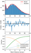 |
Fig. 2 Top: nearest neighbor distance distribution between eROSITA and eligible Gaia sources. Also shown are the best-fit model using Eq. (4) and the expected number of random matches at each distance. Middle: difference between model and data. Bottom: completeness, reliability, and contamination for samples including stars up the given match distance. |
Properties used for classification
3 Method I: support vector machine
To identify the stellar X-ray sources, we now want to classify all associations i ↔ j between eROSITA X-ray sources and eligible Gaia counterparts into the previously defined categories of stellar and non-stellar associations. This binary classification task resembles problems regularly approached with ML techniques.
The feature vector, which contains the properties describing an association i ↔ j such as the match distance rij, plays a crucial role for all ML classification methods, raising the question which features should be included in it. In principle, any combination of properties available from the Gaia and eROSITA catalogs may be used to populate the feature vector describing an association. However, the eFEDS dataset is somewhat limited in source numbers for ML methods to extract the relevant properties in the feature vector in addition to fitting or training. Therefore, we opted for an astrophysically motivated choice of properties, which are listed in Table 1. Specifically, we constructed feature vectors with MX = 2 X-ray (FX, σ) and MG = 4 Gaia features (Fg, plx, η, and BP-RP) plus the match distance rij, so that the feature vector is seven dimensional  .
.
Our choice of features has the highly advantageous property that the probability for a correct classification is a monotonic function in many features listed in Table 1. For example, an association i ↔ j1 with a Gaia source j1 being less distant (in pc) is generally the more likely counterpart than a Gaia source j2 at a larger distance when all other features are equal, because the number of chance alignments increases with distance. Similarly, the higher the optical flux, the higher is the likelihood that the association under consideration is correct, because optically bright sources are rare and, clearly, the smaller the on-sky match distance, the higher is the likelihood of a correct association. In fact, we used the latter property to strongly reduce the number of to-be-classified associations by considering only plausible ones with match distances of up to 60 arcsec.
The monotonie behavior of the feature vector with respect to the association probability makes our classification task ideally suited for a support vector machine (SVM) approach (Cortes & Vapnik 1995). A SVM classifies a feature vector pij, which in our case characterizes an association, into the two categories of stellar and non-stellar associations. The basic idea of a SVM classifier (SVC) is to use a training sample with labeled data to construct a so-called maximum-margin hyperplane separating the two categories in feature space. The confidence in the classification increases with distance from this hyperplane; samples near the hyperplane have less secure classifications compared to samples far away (in feature space) from the hyperplane. This behavior is well matched to the content of our feature vector and we used the SVC implementation of scikit-learn (Pedregosa et al. 2011) with a polynomial kernel to categorize the associations i ↔ j in the following.
3.1 Training and validation samples
The quality of the training sample is crucial for the final classification. Among the available information on the associations, the match distance stands out for indicating likely matches independent of any other property. Therefore, we constructed our final training sample in two steps, first, focusing on geometry and, second, incorporating physical properties.
3.1.1 Selection of the training sample with a geometric SVC
In a first step, we constructed a geometric training sample based on the best positional associations and some quality criterium as described in the following. The reliability of an association depends on the positional uncertainty of the X-ray source σ and on the local density of eligible counterparts η, because the expected number of random matches scales as ησ2, which must be small for a reliable association. Hence, the same match distance may be perfectly acceptable for low sky densities while unacceptable for high sky densities.
To identify the Ν best geometric associations for the final training sample, we used a geometric SVC with a feature vector consisting of match distance, positional uncertainty, and local sky density. As the geometric distributions for real and random source are known (cf. Sect. 2.2) as well as the CF, sampling from these distributions provided us with large (Ν ≳ 104) geometric training sets. These training data reproduce the geometric properties of the eFEDS field, and here we also have the labels to train the SVC. As an example, Fig. 3 shows the resulting match distance distribution for the geometric training sample, demonstrating the excellent overlap with the observed distribution in the data. The geometric SVC was then trained to classify associations based on geometry allowing a contamination of 5% spurious associations, which we found to balance sample size and contamination.
This geometric SVC was then used on the real data classifying 627 associations as real. As a cross-check, we applied the geometric SVC to randomly shifted eFEDS X-ray sources, which produces only random matches by construction. In this case, the geometric SVC classified 36 associations as stellar, which corresponds to an empirical contamination level of just under 6% well in line with the expected value.
In a second step, we applied a physical screening of the geometric training sample. In particular, we excluded associations with counterparts yielding LX > 2 × 1031 erg s−1 and empirically defined a limit of log(FX/FG) < (BP-RP) × 0.655–3.22 for the fractional X-ray fluxes of the training sample objects, larger FX/Fg-values are well above the saturation limit and unlikely to be produced by stellar coronal X-ray emission in quiescence; only highly active A-type stars may lie above the limit, but are not present in our data anyway. We further excluded a few associations with counterparts brighter than G = 5.5 mag, because they potentially cause optical loading (although the association itself may still be the correct one, just the properties could be skewed). Finally, we identified 537 bona fide stellar associations to represent the physical training sample.
This physical training sample contains, by construction, only associations with relatively small match distances, which do not sample the ensemble of expected match distances of true associations well. Therefore, we constructed the final training sample by reassigning new match distances sampling the expected distribution for real associations, just like for the geometric training sample. This time, however, we kept the X-ray and optical properties of the previously identified associations in the respective feature vectors. The final training sample also includes random associations, which were selected in proportion to the ratio implied by the CF, i.e., the training set reproduces the true ratio between real and spurious associations. The properties of random associations can be easily explored by shifting the eROSITA X-ray sources w.r.t. the background of eligible Gaia counterparts, which is what we did to incorporate them into the final training sample.
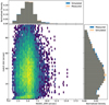 |
Fig. 3 Measured and simulated match distances for eFEDS. In the histograms, the gray bars indicate the overlap between the measured and simulated samples. |
3.1.2 Validation sample
The validation sample was constructed similarly as the random associations in the training set (see above), that is, by matching randomly shifted eFEDS sources. This validation sample contains no correct associations and all associations classified as stellar by the SVM must be spurious by construction (false positives). Usually, this procedure would give only part of the desired information, that is, would not allow an assessment of the completeness. Having an accurate estimate for the number of stellar eFEDs sources from the CF, however, provides this missing piece of information and the completeness is simply
 (7)
(7)
where N is the number of eFEDS sources with at least one association classified as stellar and Nstars = 2060 is the known number of stars from Sect. 2.2. Therefore, we do not need a validation sample containing real stellar X-ray emitters to evaluate the completeness and reliability of the classifier.
3.2 Preprocessing
Scales and ranges differ between the features used for the classification. For example, X-ray fluxes are roughly in the range of 10−14 erg s−1 cm−2 to 10−12 erg s−1 cm−2 while we considered match distances up to 60 arcsec. In such cases, it is often recommended to scale each feature to some “standardized” distribution, for example, to normalize to zero mean and standard deviation one. Empirically, however, we found that this does not provide good results for the problem at hand in terms of sample completeness and reliability. Therefore, we opted for individually scaling the features such that numerical values are roughly in the range between 0 and 10 and, e.g., used logarithmic fluxes. The exact scaling values and zero points impact the importance of individual features in the mixed terms of the polynomial kernel and may help, to some degree, to adjust their respective weights in the SVM.
3.3 Optimization goal
Classification tasks often imply a tradeoff between completeness and reliability, e.g., one may want to have a clean sample with little contamination or a sample that captures the largest number of objects at the expense of a larger contamination level. In contrast to many other classification tasks, we have a good estimate of the correct number of stars – just not which individual eROSITA sources are the stars. Therefore, we chose to optimize the classifier such that the correct number of sources are classified as stars, that is, have at least one likely stellar association. This choice implies that the number of stars misclassified as non-stellar Nmissed and the number of sources erroneously classified as stars Nspurious are equal. However, this also implies that we do not necessarily achieve the highest possible accuracy; it is conceivable that a solution exists with a larger number of correctly classified objects at the cost of, e.g., a larger imbalance between Nmissed and Nspurious. Inspecting the behavior of the SVC, we found that the hyper-parameters resulting in Nmissed = Nspurious span a well-defined path in the parameter space. From those solutions, we chose the parameters that achieve the highest accuracy.
3.4 SVC results
We used a third degree polynomial kernel and the properties from Table 1 replacing the X-ray and optical fluxes with their flux ratio FX/Fg resulting in a six dimensional feature vector. The SVC was then trained with the above described training sample and the hyper-parameters adjusted so that N = 2060 eFEDS sources are classified as stellar. With this requirement, the expected number of eROSITA sources randomly classified as stellar within the 2060 sources is Nspurious = 239 so that also Nmissed = 239 real sources are not classified as stellar by the SVC. This corresponds to a completeness and reliability of 88.4% (cf. Eqs. (5) and (6) for the definitions of completeness and reliability). The resulting sample properties will be discussed in Sect. 5 together with the sample resulting from the Bayesian approach.
The SVC does not directly provide well calibrated probabilities pij for the associations i ↔ j. Therefore, one cannot easily construct samples with different completeness or reliability values applying certain cuts in association probability pij; rather a new training run would be required to achieve the best performance for a specific completeness or reliability level. However, the number of random associations for a certain cutoff in pij can be directly derived by applying the algorithm to the validation sample. A natural choice is therefore to empirically calibrate the association probabilities pij such that
 (8)
(8)
using the validation sample. Figure 4 shows the resulting completeness and reliability levels as a function of the cutoff value pmin in the thus calibrated association probabilities pij. Here, we used the previous definitions for completeness and reliability replacing N with N>(pmin), i.e., the number of associations above the cutoff-threshold.
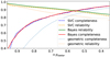 |
Fig. 4 Completeness and reliability of the stellar identifications for the eFEDS sources as a function of the probability cutoff for the SVM and Bayesian algorithms as well as the purely geometric version. |
4 Method II: Bayesian approach
In our Bayesian matching framework, the prior probability of picking by chance the correct counterpart is updated after obtaining data of the source position and properties. In that sense, we followed similar Bayesian catalog matching techniques described by Budavári & Szalay (2008) and successfully implemented in cross-matching tools such as NWAY (Salvato et al. 2018).
4.1 Distance based matching probability
Again, we consider the problem of matching NG eligible stellar candidates to NX X-ray sources. Therefore, we define the following hypotheses, the probabilities of which we want to compare:
Extending upon the scheme of Budavári & Szalay (2008), we know that only a fraction CF of the X-ray sources can be associated with one of the NG counterparts based on the distribution of the match distances rij and sky densities ηj (cf. Sect. 2.2). Hence, we derived the prior probability that none of the optical counterparts is associated with the ith X-ray source through
 (9)
(9)
and the prior probability that the jth counterpart is the identification of the ith X-ray source by
 (10)
(10)
where η is the source density in the area of the sky given by Ω.
Next, we considered the positions of the X-ray source and the eligible stellar candidates. Neglecting the positional uncertainty of the stellar candidates, the likelihood of obtaining the data Di given that the jth counterpart is the correct identification of the ith X-ray source was estimated through
 (11)
(11)
where σi is the positional uncertainty of the ith X-ray source and rij is the angular separation between the ith X-ray source and the jth counterpart (cf. Eq. (1)). Counterparts for which rij ≫ σi can be neglected based on the exponential term. Assuming the X-ray source is not associated with any of the counterparts, the likelihood of the data becomes
 (12)
(12)
In accordance with Budavári & Szalay (2008), we then obtained the geometric Bayes factor
 (13)
(13)
Applying Bayes’ theorem, we computed the posterior probability that the jth counterpart is the correct identification through
 (14)
(14)
The probability that any of the stellar counterparts is the correct identification, which is equivalent to the X-ray source being stellar given a complete and uncontaminated counterpart catalog of all and only stars, is given by
 (15)
(15)
| Hi1 | : | the ith X-ray source is associated with the j = 1 counterpart |
| ⋮ | ||
| Hij | : | the ith X-ray source is associated with the jth counterpart |
| Hi0 | : | the ith X-ray source is not associated with any of the counterparts. |
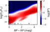 |
Fig. 5 Distribution of the Bayes factor Bp as a function of the activity FX/FG and the color BP-RP for the eFEDS counterparts. The ranges of the spectral types are indicated at the bottom of the figure. |
4.2 Consideration of additional source properties
Additional properties of the counterparts and X-ray sources can be considered to identify the best match. For example, the matching probability can be increased if the activity estimated by the X-ray flux and the optical brightness of the counterpart meets the expectations of a stellar source and few random associations are expected at such activity levels. Technically, this was achievedp by expanding the geometric Bayes factor by another factor  , which represents the expected ratio between physical associations and random associations, so that
 (16)
(16)
As additional properties, we used the X-ray to optical flux ratio, FX/FG, and the BP − RP color from Gaia.
We estimated the factor  from the data themselves. In particular, we constructed a training set of highly probable geometric counterparts. To obtain a clean training set, we selected the counterparts with a posterior geometric matching probability >0.9 only (cf. Eq. (14)). Of the thus identified 577 reliable counterparts, we expect 32 to still be spurious. Applying the same screening procedures as for the SVC training sample (cf. Sect. 3.1), we arrived at a training set with 494 bona fide coronal sources. To derive the distribution of specific properties for spurious association, we again shifted the X-ray sources arbitrarily on the fixed background of counterparts in the eFEDS field and studied the thus constructed set of explicitly random matches.
As our eFEDS training sample remains rather small, some regions in the FX/FG versus BP − RP plane are sparsely populated, which confounds the estimation of  . This affects, e.g., M-type sources at low FX/FG values, which are reasonable X-ray emitters by physical standards, but are unlikely to be detected in X-rays at the eFEDS sensitivity. Therefore, we adopted a value of one for
  in this region of inactive M-dwarfs. On the other end of the main sequence, early A- and B-type stars with high FX/FG values can be excluded as true identifications based on physical grounds, here
  goes to zero, which is tantamount to assuming that essentially all such matches are random associations. Nonetheless, for most of the counterparts, the details of the estimation of
  have minor impact on the derived matching probabilities.
In Fig. 5, we show the resulting map of Bayes factors  for the eFEDS counterparts. For example, F-type sources with an activity level of around log(FX/FG) ≈ −5 are weighted up, while counterparts with log(FX/FG) > −2 are weighted down by considering the additional properties. The Bayes map generally appears rather smooth. However, regions of the Bayes map sparsely populated by training and control sources may show some distinct structure, in particular the increase of the Bayes factor for sources around BP − RP = 2.2 mag and log FX/FG = −5. The influence of these “low source density regions” on our identifications is marginal because the number of counterparts in these regions is also very small and in fact, neither the SVM nor the methods described in Salvato et al. (2022) show an excess or deficit of sources in this part of the diagram when compared to the Bayesian method (see Fig. 6). We also note that although sources with high X-ray to optical flux ratios are excluded from the training set, such sources can nevertheless be identified in the final sample if their positional match is good or the number of expected spurious association with such properties is small, because then the Bayes factor
  . is still about unity.
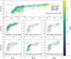 |
Fig. 6 Ratio between X-ray and G-band fluxes as a function of the associated Gaia object’s BP-RP color. The objects are colored according to the parallax. The label in the lower part of all seven panels indicate in which sample the colored objects belong: SVM, Bayes, and Salvato describe the method and “!” equals not, that is, that the colored identification are not identified by the method that is preceded by the “!”. The number in bracket indicates the respective number of sources. In rows two and three, the gray dots represent the objects of the top panel for reference. The dotted line in the bottom row indicates log LX/Lbol = −2.5. |
4.3 Bayesian results
Applying the matching procedure described in Sects. 4.1 and 4.2, we obtained a stellar probability for every eFEDS source. In contrast to the SVC, these probabilities are well calibrated so that the completeness and reliability of a sample resulting from choosing a specific probability threshold can be derived directly. The expected number of missed (false negatives) and spurious (false positives) stellar identification is estimated through
 (17)
(17)

where N> and N< are the number of sources above and below the threshold and their probabilities are denoted by pstellar,> and pstellar,<, respectively. Completeness and reliability of the obtained sample were estimated through Eqs. (5) and (6) by replacing Ν with N>.
In Fig. 4 we present the expected completeness and reliability obtained with the Bayesian approach as a function of the stellar probability cutoff. At pstellar ≈ 0.58 the expected number of stellar sources in the eFEDS field is recovered, here, about 11% of the identifications are expected to be spurious and the same fraction of stellar eFEDS sources is expected to be missed. Going to larger stellar probabilities, the completeness decreases and the reliability increases, as expected. We note that these values were empirically verified by applying our Bayesian identification procedure to arbitrarily shifted eFEDS sources similar to the SVC test sample.
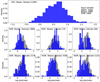 |
Fig. 7 Histograms for the parallaxes of the identified Gaia counterparts. Individual panels as in Fig. 6. The parallax distribution of the associations identified by all three methods (top panel) is shown in the background as the gray histogram in the middle and bottom rows. |
5 Results and comparison between approaches
We are interested in the physical properties of the stars detected by eROSITA, more precisely, in the resulting association properties. Therefore, we base our comparison on associations and not on the classification of an eROSITA source as stellar; a discussion of the overlap in stellar classifications is provided in Salvato et al. (2022).
5.1 Comparison samples
To compare the samples identified by the different methods, we cut the SVM and Bayesian catalogs in pij such that 2060 eROSITA sources are classified as stellar. We also include the catalog presented in Salvato et al. (2022), which provides counterparts to all eFEDS sources regardless of their galactic or extra galactic nature. These authors used a training sample of 23 000 XMM-Newton and Chandra sources with secure counterparts and the final counterpart identification is done after comparing the associations obtained with NWAY (Salvato et al. 2018) with a modified version of Maximum Likelihood (Sutherland & Saunders 1992) as described in Ruiz et al. (2018). Again, we cut their sample of stellar sources in pany to obtain 2060 stellar eROSITA sources. Furthermore, we mapped their Gaia DR2 IDs to EDR3 IDs for the comparison noting that not all DR2 sources could be unambiguously mapped to a EDR3 source.
The SVM and Bayesian approaches perform about equally well with an overlap of 1873 associations in both samples (91%). This fraction incidentally coincides with the expected reliability of the respective samples. Therefore, it is possible albeit unlikely that all true associations are among the shared associations and that all spurious associations are being identified by one method alone. The resulting sample properties in terms of completeness and reliability are very similar for the SVM and Bayesian approaches (see Fig. 4). The differences are compatible with the Poisson noise for the number of missed or spurious sources at the respective probability thresholds.
The overlap between the results by Salvato et al. (2022) and the SVM and Bayesian approaches is smaller with about 1550 and 1558 associations in common, respectively. This smaller overlap is partly caused by the different Gaia data releases (145 associations are affected) and by the construction of the sample since we cut the sample to the 2060 “best” associations. The overlap in stellar classifications of eROSITA sources is much higher (cf. Salvato et al. 2022).
5.2 Sample properties
We show the physical properties of the resulting samples in Figs. 6 to 9. Figures 6 to 8 display different properties but their structure is identical. They all contain seven panels organized in three rows: The first row shows the properties of the associations overlapping between all three methods (1484 in total). The second row shows the properties of the associations overlapping between only two methods and we present one panel for each of the possible combinations. For each panel, we provide an annotation indicating which sample(s) contain the displayed associations. We use a “!” to indicate that the associations are not in the sample following the “!”, for example, the left panel in the second row with the SVM, Bayes, !Salvato annotation implies that the associations are in the SVM and Bayesian samples but not among the 2060 best Salvato et al. (2022) stellar associations. Finally, the third row shows the associations exclusively contained in only one sample. To ease the comparison between the different samples, we display in rows two and three of Figs. 6 to 8 the associations overlapping between all three methods (shown in the top panel of each figure) in the background (in gray). Numbers in brackets following the sample description indicate the number of associations (displayed in color).
Figure 6 shows that the Fx/Fg distributions are relatively similar for all identification methods. Noticeable is that all methods classify some associations above the saturation limit of log LX/Lbol = −3 as stellar (gray dashed line in Fig. 6). These associations between an eROSITA source and a Gaia source have a combination of high positional match likelihoods and are, for SVC, relatively nearby, which counterbalances the high FX/FG-values and lead to the stellar classification. At least some cases of unusually high Fx/Fg values result from flaring: 65 variable sources are discussed in Boller et al. (2022). Most of these variable sources are associated with stars and show X-ray light curves resembling the typical shape of flaring due to magnetic activity when sufficient X-ray coverage is available. Furthermore, most sources are within 0.5 dex of the boundary for all methods (dashed line in Fig. 6). The methods employed by Salvato et al. (2022) identify a small number of sources (~10) with Gaia sources leading to quite high Fx/Fg values, probably because their association is based on characterizing the entire SED. In total, the number of sources above the saturation limit remains small: neither method associates more than hundred eFEDS sources with a Gaia source leading to Fx/Fg values implying X-ray emission above the saturation limit (< 5% of the stellar classifications).
Overall the associations classified as stellar fall within the expected BP-RP-color vs Fx/Fg range of stellar sources for all three methods. The main features are (a) high X-ray activity levels for M dwarfs close to the saturation level, (b) a substantial spread in X-ray activity for stars of spectral types F to early K, and (c) the onset of magnetic activity at late A/early F spectral types. These properties are also seen for the sample of stellar X-ray sources in the XMM-Newton slew survey catalog identified by Freund et al. (2018) and may be a general property of flux limited X-ray surveys.
We show in Fig. 9 the positions of the Gaia sources associated with the stellar eROSITA sources in a color-magnitude diagram. By construction, the associated Gaia sources are compatible with young to main sequence stars as well as stars of moderate age (in the few Gyr range). Differences between the SVM and Bayesian method are small and the identified Gaia sources are largely overlapping in the HRD. As expected, the distances towards the earlier spectral types tend to be larger than towards the later spectral types, in particular M dwarfs, which are found within about 200 pc. Both methods associated stars on the red giant branch with eROSITA sources. These sources may not be causing the X-ray emission as red giants beyond a so-called dividing line have been found to lack genuine X-ray emission (Haisch et al. 1991). We note, however, that (a) lower-mass companions may be responsible for the detected X-ray emission and (b) the association likelihoods of these sources are indeed quite low. In particular, the reddest giant in Fig. 9 (HT Hya) is also a GALEX FUV and NUV source with pstellar ≈ 0.7, i.e., this source may very well be the correct association although the giant itself may not dominate the X-ray emission. Nevertheless, we purposely keep these sources (and potentially other source classes) in the final sample to avoid biasing ourselves unduly towards current “wisdom” precluding new discoveries.
The parallax-distributions (Fig. 7) show that the identified stellar sources peak between log plx = 0.5 and log plx = 1, i.e., are mostly between 100 pc and 250 pc from the Sun. Few sources are farther than 1kpc (log plx <0). The objects associated by the Bayesian method and Salvato et al. (2022) tend to have smaller parallaxes (larger distances) compared to the SVC. For the Bayesian method, this may be expected, because it is currently ignorant of the Gaia parallaxes. Salvato et al. (2022) do consider the parallax in their method, but it likely has a different (lower) importance than for the SVC, which can use the parallax information to boost the association likelihood of certain associations (see red dots in Fig. 10). In theory, the parallax information may be beneficially used to reduce the number of spurious associations as the number of possible random associations increases with distance. At the moment, however, the SVC is not able to take full advantage of this benefit resulting in similar reliability and completeness levels as the Bayesian approach, probably because of the limited training set.
Lastly, the match distance-distribution shows that the associations identified as stellar by all three methods have, on average, the smallest match distances (cf. Fig. 8). The stellar associations shared between the Bayesian and SVC methods have relatively small match distances, too. The other panels of Fig. 8, however, show that the match distances tend to be larger for associations found by only one method. For these associations, the positional match is insufficient to result in a secure stellar identification and the weighting of the other features becomes important, which is different between the three methods.
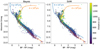 |
Fig. 9 Color-magnitude diagrams for the identified stellar sources (left: Bayes, right: SVM). The color indicates the distance of the sources. Isochrones are shown for two representative stellar ages of 4 × 10⁷ and 4 × 10⁹ yr using the PARSEC isochrones (Bressan et al. 2012). |
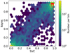 |
Fig. 10 Association probabilities for the SVC and Bayesian methods. The red dots depict the sources within 100 pc. |
5.3 Probabilities
Our Bayesian and SVC methods were developed focusing on stars (coronal emitters). Therefore, we compare the calculated probabilities from the SVC and Bayesian methods in Fig. 10 (after calibrating the SVC probabilities as described in Sect. 3.4). Overall, the probabilities are very similar being clustered around the 1:1 relation, most sources get either very low or high association probabilities in both methods. In addition to some intrinsic scatter, a number of sources get relatively high association probabilities by the SVC method while the Bayesian method assigns only mediocre probabilities between 0.5 and 0.8 (the structure located in the right middle part of Fig. 10. Most of these sources are within 100 pc (red dots in Fig. 10) so that they get boosted association probabilities due to these high parallax-values compared to the Bayesian approach, which currently ignores the parallaxes.
5.4 HamStar catalog
The catalog of the stellar sources is based on the Bayesian framework, because it directly provides probabilities reflecting our prior knowledge and the data. We also include two columns that indicate if the particular association is also identified by the SVM approach and in the catalog by Salvato et al. (2022). This catalog is dubbed “HamStars” in the eROSITA context.
6 Conclusions and outlook
We present SVM and Bayesian methods specifically designed to identify stars among the eROSITA sources. The two methods provide very similar results, both, in terms of sample quality (completeness and reliability) and resulting physical properties. Both methods provide significant improvements over a purely geometric approach reducing the number of spurious associations in the sample by about a factor of two and samples constructed to contain the geometrically expected number of eROSITA sources achieve almost 90% completeness and reliability. Furthermore, we show how to construct calibrated probabilities for both methods, which can be eventually used to create sub-samples with specific completeness and reliability properties by applying appropriate cuts in association probability.
On the one hand, it is somewhat surprising that the SVM and Bayesian methods perform so similarly, because the SVM method uses the parallax measurement as an additional information compared to the Bayesian approach. On the other hand, the SVM method is ignorant of the “mathematics” of the matching distance and needs to learn the positional match characteristics from the training sample. We expect that a larger training sample will, at least partly, mitigate this issue, in particular when applied to the eROSITA all-sky survey (eRASS).
The sample quality in terms of completeness and reliability is specific to eFEDS, because these properties depend on (a) the depth of the X-ray exposure, (b) the ratio between stellar and other X-ray sources, and (c) the sky density of the eligible stellar counterparts. These properties are expected to change strongly with galactic position, e.g. the sky density of eligible stellar counterparts differs by at least a factor of hundred between the galactic pole and bulge regions. Therefore, these effects need to be taken into account to achieve similar or better results for eRASS compared to eFEDS. In the future, we plan to also include additional information from the X-ray data such as spectral hardness to further improve the algorithms for their application to eRASS. Lastly, future Gaia data releases will improve the quality of the match catalog. We are therefore confident that it is possible to construct well characterized stellar samples from eROSITA data. Such a large sample of stars with well known X-ray properties will allow us to improve our understanding of stellar activity throughout space and time.
Acknowledgements
eROSITA is the primary instrument aboard SRG, a joint Russian-German science mission supported by the Russian Space Agency (Roskosmos), in the interests of the Russian Academy of Sciences represented by its Space Research Institute (IKI), and the Deutsches Zentrum für Luft-und Raumfahrt (DLR). The SRG spacecraft was built by Lavochkin Association (NPOL) and its subcontractors, and is operated by NPOL with support from IKI and the Max Planck Institute for Extraterrestrial Physics (MPE). The development and construction of the eROSITA X-ray instrument was led by MPE, with contributions from the Dr. Karl Remeis Observatory Bamberg and ECAP (FAU Erlangen-Nürnberg), the University of Hamburg Observatory, the Leibniz Institute for Astrophysics Potsdam (AIP), and the Institute for Astronomy and Astrophysics of the University of Tübingen, with the support of DLR and the Max Planck Society. The Argelander Institute for Astronomy of the University of Bonn and the Ludwig Maximilians Universität Munich also participated in the science preparation for eROSITA. This work has made use of data from the European Space Agency (ESA) mission Gaia (https://www.cosmos.esa.int/gaia), processed by the Gaia Data Processing and Analysis Consortium (DPAC, https://www.cosmos.esa.int/web/gaia/dpac/consortium). Funding for the DPAC has been provided by national institutions, in particular the institutions participating in the Gaia Multilateral Agreement. PCS gratefully acknowledges support by the DLR under 50 OR 1901 and 50 OR 2102. SF acknowledges supports through the Integrationsamt Hildesheim, the ZAV of Bundesagentur für Arbeit, and the Hamburg University and thanks Gabriele Uth and Maria Theresa Lehmann for their support.
Appendix A Isochrones
Figure A.1 shows the region in which a Gaia source is considered an eligible stellar counterpart.
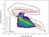 |
Fig. 11 Polygon containing valid stellar sources with PARSEC evolutionary tracks. The 2D histogram in the background shows a typical Gaia source population; most sources are close to the 100+ Myrs main sequence. |
References
- Binder, D. A. 1978, Biometrika, 65, 31 [CrossRef] [Google Scholar]
- Boller, T., Schmitt, J. H. M. M., Buchner, J., et al. 2022, A&A, 661, A8 (eROSITA EDR SI) [NASA ADS] [CrossRef] [EDP Sciences] [Google Scholar]
- Bressan, A., Marigo, P., Girardi, L., et al. 2012, MNRAS, 427, 127 [NASA ADS] [CrossRef] [Google Scholar]
- Brunner, H., Liu, T., Lamer, G., et al. 2022, A&A, 661, A1 (eROSITA EDR SI) [NASA ADS] [CrossRef] [EDP Sciences] [Google Scholar]
- Budavári, T., & Szalay, A. S. 2008, ApJ, 679, 301 [CrossRef] [Google Scholar]
- Cortes, C., & Vapnik, V. 1995, Mach. Learn., 20, 273 [Google Scholar]
- Fischer, R. A. 1938, Ann. Eugen., 8, 376 [CrossRef] [Google Scholar]
- Freund, S., Robrade, J., Schneider, P. C., & Schmitt, J. H. M. M. 2018, A&A, 614, A125 [NASA ADS] [CrossRef] [EDP Sciences] [Google Scholar]
- Gaia Collaboration (Prusti, T., et al.) 2016, A&A, 595, A1 [NASA ADS] [CrossRef] [EDP Sciences] [Google Scholar]
- Gaia Collaboration (Brown, A. G. A., et al.) 2021, A&A, 649, A1 [NASA ADS] [CrossRef] [EDP Sciences] [Google Scholar]
- Gilmore, G., Randich, S., Asplund, M., et al. 2012, The Messenger, 147, 25 [NASA ADS] [Google Scholar]
- Güdel, M. 2004, A&ARv, 12, 71 [CrossRef] [Google Scholar]
- Haisch, B., Schmitt, J. H. M. M., & Rosso, C. 1991, ApJ, 383, L15 [NASA ADS] [CrossRef] [Google Scholar]
- Liu, T., Buchner, J., Nandra, K., et al. 2022, A&A, 661, A5 (eROSITA EDR SI) [NASA ADS] [CrossRef] [EDP Sciences] [Google Scholar]
- Marton, G., Abraham, P., Szegedi-Elek, E., et al. 2019, MNRAS, 487, 2522 [CrossRef] [Google Scholar]
- Melton, E. 2020, AJ, 159, 200 [NASA ADS] [CrossRef] [Google Scholar]
- Merloni, A., Predehl, P., Becker, W., et al. 2012, ArXiv e-prints, [arXiv:1289.3114] [Google Scholar]
- Pedregosa, F., Varoquaux, G., Gramfort, A., et al. 2011, J. Mach. Learn Res., 12, 2825 [Google Scholar]
- Pizzolato, N., Maggio, A., Micela, G., Sciortino, S., & Ventura, P. 2003, A&A, 397, 147 [NASA ADS] [CrossRef] [EDP Sciences] [Google Scholar]
- Predehl, P., Andritschke, R., Arefiev, V., et al. 2021, A&A, 647, A1 [EDP Sciences] [Google Scholar]
- Ruiz, A., Corral, A., Mountrichas, G., & Georgantopoulos, I. 2018, A&A, 618, A52 [NASA ADS] [CrossRef] [EDP Sciences] [Google Scholar]
- Salvato, M., Buchner, J., Budavári, T., et al. 2018, MNRAS, 473, 4937 [Google Scholar]
- Salvato, M., Wolf, J., Dwelly, T., et al. 2022, A&A, 661, A3 (eROSITA EDR SI) [NASA ADS] [CrossRef] [EDP Sciences] [Google Scholar]
- Schmitt, J. H. M. M., & Liefke, C. 2004, A&A, 417, 651 [NASA ADS] [CrossRef] [EDP Sciences] [Google Scholar]
- Skumanich, A. 1972, ApJ, 171, 565 [Google Scholar]
- Steinmetz, M., Zwitter, T., Siebert, A., et al. 2006, AJ, 132, 1645 [Google Scholar]
- Sutherland, W., & Saunders, W. 1992, MNRAS, 259, 413 [Google Scholar]
- Testa, P., Saar, S. H., & Drake, J. J. 2015, Philos. Trans. Roy. Soc. London A, 373, 20140259 [NASA ADS] [Google Scholar]
- Vilhu, O. 1984, A&A, 133, 117 [NASA ADS] [Google Scholar]
- Vioque, M., Oudmaijer, R. D., Schreiner, M., et al. 2020, A&A, 638, A21 [NASA ADS] [CrossRef] [EDP Sciences] [Google Scholar]
- Vulic, N., Hornschemeier, A. E., Haberl, F., et al. 2022, A&A, 661, A16 (eROSITA EDR SI) [NASA ADS] [CrossRef] [EDP Sciences] [Google Scholar]
- Wright, N. J., Drake, J. J., Mamajek, E. E., & Henry, G. W. 2011, ApJ, 743, 48 [Google Scholar]
A RUWE value of 1.4 was suggested for single stars within 100 pc, see http://www.rssd.esa.int/doc_fetch.php?id=3757412
All Tables
All Figures
|
Fig. 1 Limiting G magnitude for stars emitting at X-ray activity levels of log LX/Lbol = −2.5 and −3 assuming the average eFEDS exposure depth. |
| In the text | |
|
Fig. 2 Top: nearest neighbor distance distribution between eROSITA and eligible Gaia sources. Also shown are the best-fit model using Eq. (4) and the expected number of random matches at each distance. Middle: difference between model and data. Bottom: completeness, reliability, and contamination for samples including stars up the given match distance. |
| In the text | |
|
Fig. 3 Measured and simulated match distances for eFEDS. In the histograms, the gray bars indicate the overlap between the measured and simulated samples. |
| In the text | |
|
Fig. 4 Completeness and reliability of the stellar identifications for the eFEDS sources as a function of the probability cutoff for the SVM and Bayesian algorithms as well as the purely geometric version. |
| In the text | |
|
Fig. 5 Distribution of the Bayes factor Bp as a function of the activity FX/FG and the color BP-RP for the eFEDS counterparts. The ranges of the spectral types are indicated at the bottom of the figure. |
| In the text | |
|
Fig. 6 Ratio between X-ray and G-band fluxes as a function of the associated Gaia object’s BP-RP color. The objects are colored according to the parallax. The label in the lower part of all seven panels indicate in which sample the colored objects belong: SVM, Bayes, and Salvato describe the method and “!” equals not, that is, that the colored identification are not identified by the method that is preceded by the “!”. The number in bracket indicates the respective number of sources. In rows two and three, the gray dots represent the objects of the top panel for reference. The dotted line in the bottom row indicates log LX/Lbol = −2.5. |
| In the text | |
|
Fig. 7 Histograms for the parallaxes of the identified Gaia counterparts. Individual panels as in Fig. 6. The parallax distribution of the associations identified by all three methods (top panel) is shown in the background as the gray histogram in the middle and bottom rows. |
| In the text | |
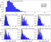 |
Fig. 8 Histograms for the match distance to the associated Gaia counterparts. Similar to Fig. 7. |
| In the text | |
|
Fig. 9 Color-magnitude diagrams for the identified stellar sources (left: Bayes, right: SVM). The color indicates the distance of the sources. Isochrones are shown for two representative stellar ages of 4 × 10⁷ and 4 × 10⁹ yr using the PARSEC isochrones (Bressan et al. 2012). |
| In the text | |
|
Fig. 10 Association probabilities for the SVC and Bayesian methods. The red dots depict the sources within 100 pc. |
| In the text | |
|
Fig. 11 Polygon containing valid stellar sources with PARSEC evolutionary tracks. The 2D histogram in the background shows a typical Gaia source population; most sources are close to the 100+ Myrs main sequence. |
| In the text | |
Current usage metrics show cumulative count of Article Views (full-text article views including HTML views, PDF and ePub downloads, according to the available data) and Abstracts Views on Vision4Press platform.
Data correspond to usage on the plateform after 2015. The current usage metrics is available 48-96 hours after online publication and is updated daily on week days.
Initial download of the metrics may take a while.