| Issue |
A&A
Volume 661, May 2022
The Early Data Release of eROSITA and Mikhail Pavlinsky ART-XC on the SRG mission
|
|
|---|---|---|
| Article Number | A20 | |
| Number of page(s) | 7 | |
| Section | Stellar structure and evolution | |
| DOI | https://doi.org/10.1051/0004-6361/202141082 | |
| Published online | 18 May 2022 | |
SRG/eROSITA discovery of 164 s pulsations from the SMC Be/X-ray binary XMMU J010429.4-723136
1
Max-Planck-Institut für extraterrestrische Physik,
Gießenbachstraße 1,
85748
Garching, Germany
e-mail: This email address is being protected from spambots. You need JavaScript enabled to view it.
2
Leibniz Institut für Astrophysik Potsdam,
An der Sternwarte 16,
14482
Potsdam, Germany
3
South African Astronomical Observatory,
PO Box 9, Observatory,
Cape Town 7935, South Africa
4
Department of Astronomy, University of Cape Town,
Private Bag X3, 7701
Rondebosch, South Africa
Received:
14
April
2021
Accepted:
18
October
2021
Abstract
Context. The Small Magellanic Cloud (SMC) hosts many known high-mass X-ray binaries (HMXBs), and all but one (SMC X-1) have a Be companion star. Through the calibration and verification phase of eROSITA on board the Spektrum-Roentgen-Gamma (SRG) spacecraft, the Be/X-ray binary XMMU J010429.4-723136 was in the field of view during observations of the supernova remnant, 1E0102.2-7219, used as a calibration standard.
Aims. We report timing and spectral analyses of XMMU J010429.4-723136 based on three eROSITA observations of the field, two of which were performed on 2019 November 7-9, with the third on 2020 June 18-19. We also reanalyse the OGLE-IV light curve for that source in order to determine the orbital period.
Methods. We performed a Lomb-Scargle periodogram analysis to search for pulsations (from the X-ray data) and for the orbital period (from the OGLE data). X-ray spectral parameters and fluxes were retrieved from the best-fit model.
Results. We detect, for the first time, the pulsations of XMMU J010429.4-723136 at a period of -164 s, and therefore designate the source as SXP 164. From the spectral fitting, we derive a source flux of ~1 × 10⁻¹² erg s−1 cm−2 for all three observations, corresponding to a luminosity of ~4 × 1035 erg s−1 at the distance of the SMC. Furthermore, reanalysing the OGLE light curve, including the latest observations, we find a significant periodic signal that we believe is likely be the orbital period; at 22.3 days, this is shorter than the previously reported values. The Swift/XRT light curve, extracted from two long monitorings of the field and folded at the same period, suggests that a modulation is also present in the X-ray data.
Key words: galaxies: individual: Small Magellanic Could / stars: neutron / X-rays: binaries / X-rays: individuals: SXP 164 / stars: emission-line, Be
© S. Carpano et al. 2022
 Open Access article, published by EDP Sciences, under the terms of the Creative Commons Attribution License (https://creativecommons.org/licenses/by/4.0), which permits unrestricted use, distribution, and reproduction in any medium, provided the original work is properly cited.
Open Access funding provided by Max Planck Society.
1 Introduction
High-mass X-ray binaries (HMXBs) are binary systems composed of an early-type star and a compact object that is either a neutron star or a black hole (occasionally a white dwarf). Be or B[e]-type stars are a subset of B-type stars where one or more Balmer emission lines are found in the optical spectrum. They are believed to possess an equatorial decretion disc, possibly causing regular X-ray outbursts at periastron passage of the compact object due to enhanced mass accretion (see e.g. Reig 2011, for a review). A large number of such systems were found in the Small Magellanic Cloud (SMC). The latest comprehensive catalogue was published by Haberl & Sturm (2016) and collects 121 high-confidence HMXBs (the vast majority with Be companion stars). For about half of the sample, X-ray pulsations were discovered with periods ranging from a fraction of a second to a few thousand seconds. Pulse periods of the 62 Be/X-ray binaries have a bimodal distribution peaking at around 10 s and 250 s (Haberl & Sturm 2016). For the other sources, pulse periods are still not reported, one of them being XMMU J010429.4–723136, identified as source number 132 in Table A.1 of this latter publication. The source was already mentioned as source number 3285 in the previous XMM-Newton catalogue of X-ray point sources in the SMC (Sturm et al. 2013, their Table 5).
XMMU J010429.4–723136 was confirmed as a Be star (more precisely of type B1V) by McBride et al. (2017) based on spectra recorded with the Anglo-Australian Telescope on 2012 July 7–8 in the wavelength range [4025–4775] Å. Large X-ray variability had previously been reported by Maggi et al. (2013) comparing a series of Swift/XRT observations, where the luminosity ranged from 2.8 to 12.4 × 1035 erg s−1 on MJD 56627.09 to 56643.31 (2013 December), with a previous XMM-Newton observation on MJD 55 149.1 (2009 November), where only an upper limit a factor of ~400 lower could be extracted. The source is not reported in the RXTE catalogue of SMC pulsars from Galache et al. (2008) based on 9 yr of SMC survey (starting in 1997), but was detected by Chandra in 2002 August with a luminosity of 1.4 × 1035 erg s−1 (Rajoelimanana et al. 2011a).
The Optical Gravitational Lensing Experiment (OGLE) light curve of XMMU J010429.4–723136 in the I-band is shown in McBride et al. (2017) as source XMM 3285, covering the epoch from MJD 55 346 to MJD ~57400 (2010 May to 2016 January). The source was in a low state for ~600 days and then increased towards a stable higher state (∆I = 1.25 mag). A period of 29.75 days was found in the data covering the short time interval MJD 55 650–56 100 (and after some detrending). This is somewhat lower than the strong modulation of 37.15 ± 0.02 days claimed by Rajoelimanana et al. (2011a) and associated later by Schmidtke et al. (2013), with aliasing of a possible shorter period modulation of 0.972 days. This last short period was interpreted as non-radial pulsations from the Be star. We note that in both works from Rajoelimanana et al. (2011a) and Schmidtke et al. (2013), the source is erroneously named SXP 707 from a period discovered in the Chandra data at 707 s. That period is, in reality, the satellite dithering period, with the source located at the rim of a CCD, moving in and out of the detector (as already clarified by Haberl & Sturm 2016).
In this paper, we report the discovery of X-ray pulsations for XMMUJ010429.4–723136 with a period of 164 s and rename the source SXP 164 following the terminology first proposed by Coe et al. (2005) (where SXP stands for Small Magellanic Cloud X-ray Pulsar, followed by the pulse period in seconds to three significant figures). The discovery was briefly announced by Haberl et al. (2019). We also report the detection of a strong signal at 22.3 days in the OGLE-IV light curve that we interpret as the possible orbital period.
2 Observations and data reduction
X-ray observations were performed during the calibration and verification phase of eROSITA (Predehl et al. 2021), from UTC 2019 November 07 17:13:18 to 2019 November 08 09:53:18 (ObsID 700001) and 2019 November 09 02:41:38 to 2019 November 09 19:21:38 (ObsID 700003), each observation for a total exposure of ~60ks. A third observation occurred half a year later from 2020 June 18 19:43:25 to 2020 June 19 06:00:41 (~37 ks, ObsID 710 000). During the first observation, the source was far off-axis (at an angle of 29.8’) and was covered by only four cameras, telescope modules TM1,4,5,6 (for TM3, as only a small fraction of the PSF lies in the field of view, the data are not included in the analysis). Instead, the source was located in the field of view of all seven cameras in the second and third observations (with an off-axis angle of 26.8’ and 28.4’, respectively). The data were reduced using the eROSITA Standard Analysis Software System pipeline (eSASS; Brunner et al. 2022) version eSASSusers_201009. The software determines good time intervals, corrupted events and frames, and dead times, and masks bad pixels, projects the photons onto the sky, and applies pattern recognition and energy calibration. Source and background extraction regions were defined as an ellipse and an elliptical annulus, respectively. The regions were centred on the XMM-Newton coordinates of the source (RA, Dec)= (01:04:29.42,-72:31:36.5), derived in Sturm et al. (2013). For the observation 700 001, an elliptical nearby background region was selected instead as the source is observed far off-axis.
Optical spectroscopy of XMMUJ010429.4–723136 was undertaken on 2019-11-24 using the Robert Stobie Spectrograph (RSS, Burgh et al. 2003) on the Southern African Large Telescope (SALT, Buckley et al. 2006) under the transient follow-up program. The PG2300 VPH grating was used, which covered the spectral region 6100-6900 Å at a resolution of 1.2 Å. A single 1200 s exposure was obtained, starting at 19:40:08 UTC.
The X-Ray variables OGLE Monitoring (XROM) system provides real-time photometry (I-band) of optical counterparts of X-ray sources1 located in the fields observed in the oGlE-IV survey (Udalski 2008), with roughly daily sampling. To date, data available for SXP 164 cover the period from MJD 55 346 (2010-05-30) to MJD 58 870 (2020-01-21).
 |
Fig. 1 eROSITA light curve of SXP 164, during ObsID 700 001 (top), 700 003 (middle) and 710 000 (bottom), rebinned at 2000 s, extracted in the 0.2–5.0 keV band. The red lines indicate the mean values of 0.10, 0.12, and 0.16 cts s−1 for the three respective observations. |
 |
Fig. 2 Lomb-Scargle periodogram for the three eROSITA observations (top: ObsID 700 001, middle: 700 003 and bottom: 710 000), using light curves binned at 2 s. The best periods are 163.93 s, 163.85 s, and 163.48 s, respectively. |
3 Data analysis and results
3.1 eROSITA
3.1.1 X-ray light curves and pulse period search
The background-subtracted and vignetting-corrected light curves of SXP 164 from the three observations performed during the calibration phase are shown in Fig. 1. These were produced using the eSASS task srctool in the energy band 0.2–5.0 keV and with a bin size of 2000 s. The mean count rates, shown by the red lines, are 0.10, 0.12, and 0.16 cts s−1, for the three respective observations. The portion of the light curves where all available cameras are operating simultaneously has almost the same length for the first two observations (~ 17 h) and is much shorter for the third one (~10h). No large variability is observed during the individual observations.
The pulse period search is performed using a Lomb-Scargle analysis (Lomb 1976; Scargle 1982) in the energy band 0.2–5 keV (as the signal is stronger than in the 0.2–10 keV band) and in the period range 120–200 s (a larger period interval was initially used during the first screening). Figure 2 shows the periodogram corresponding to the three observations, performed on background-subtracted light curves binned at 2 s. Strong peaks are found with maxima at 163.93 s, 163.85 s, and 163.48 s, respectively. The confidence levels (given at 68%, 90%, and 99%) are derived using the block-bootstrap method as explained in Carpano et al. (2017). The analysis consists first in simulating 1000 light curves, each by splitting the original light curves into blocks of ~650 s and randomly shuffling the blocks, and then retrieving the corresponding periodogram maxima. We also performed a joint period search on the first two data sets as the values are very close, and we find the best period at 163.89 s. To estimate the uncertainty on the pulse periods, we carried out Monte Carlo simulations, similarly to what is done in Gotthelf et al. (1999), and generated a set of 1000 light curves for each observation. The block-bootstrapped light curves are used to recreate the noise while the signal is represented by a sine function whose amplitude is retrieved from the folded light curves (and the period, assumed to be constant, from the maxima of the periodograms). In that way, the significance of the peak in the periodograms derived from the simulated data is about the same as with the original light curves. The corresponding measured periods are well represented by a normal distribution and the mean values are very close to the input periods (163.926s, 163.848 s, and 163.489 s). The standard deviation of the distribution is taken as the 1 σ uncertainty in the period and is 0.042 s, 0.030 s, and 0.051 s, for the three observations, respectively. The uncertainty on the period retrieved by merging the first two data sets is 0.007 s (for a mean value of 163.897 s).
Figure 3 shows the folded light curves of SXP 164 with the best fit sine functions overlaid. For the first two observations, they are folded at their common period (163.89 s), while the third one is folded at its own best period. The light curves are phase connected with phase ‘0’ being the start of the first observation. The pulse profile of the second observation looks less sinusoidal than that of the third one (the first one is more noisy as less photons are available). The reduced chi-square of the sine fit (defined as  /d.o.f. with obsi being the folded rate, fit the sine function, σi the rate errors, and d.o.f. the degrees of freedom) is 1.7, 5.4, and 2.3 for the three respective observations. On the other hand, the pulsed fraction (defined as
  × 100 (%), with max and min being the maximum and minimum of the folded light curves) is 64%, 78%, and 73% for the first, second and third observation, respectively.
 |
Fig. 3 Folded eROSITA light curves of SXP 164 during ObsID 700 001 (top), 700003 (middle), and 710 000 (bottom), extracted in the 0.2–5.0 keV band. The best-fit sine function is overlaid. Phase 0 corresponds to the start of the first observation. The light curves from the first two observations are folded with the common period (163.89 s). |
 |
Fig. 4 Simultaneous spectral fit of SXP 164 using an absorbed power-law model (TBabs*TBvarabs*power), and the corresponding residuals for ObsID 700 001 (3 cameras) and 700 003 (5 cameras) at the top and ObsID 710 000 (5 cameras) at the bottom. |
3.1.2 Spectral analysis
For all three observations, the eROSITA spectra of SXP 164 were fitted with PyXspec2 in the full 0.2–10keV energy band, and for the first two observations simultaneously (fitting the data for the two observations separately would lead to similar spectral parameters but with larger uncertainties). The spectra for all cameras covering the sources (excluding the light-leak cameras TM5 and TM7, Predehl et al. 2021) were fitted using an absorbed power law and two absorption components (TBabs*TBvarabs*power). TBabs and TBvarabs are the Tuebingen-Boulder interstellar medium (ISM) absorption models as defined in Wilms et al. (2000). The first absorption component has a fixed Galactic NH value of 5.36 × 1020 cm−2 (Dickey & Lockman 1990) and the second NH is left free, while the abundance is fixed to 1.0 for He and 0.2 for Z > 2 (Russell & Dopita 1992). The second X-ray absorption component arises in the ISM of the SMC or close to the source.
For the first two observations, only the normalisation constant for the spectra of different observations was left free. The results of the spectral fit are shown in Fig. 4 together with their residuals, for ObsID 700001 and 700003 (top), and 710000 (bottom). The values of the spectral parameters as well as the observed and unabsorbed fluxes and luminosities (assuming a distance of 60.6 kpc, Hilditch et al. 2005) are shown in Table 1. The observed fluxes are in the range of those reported by Maggi et al. (2013), 0.66–2.87 × 10⁻¹² erg cm−2 s−1, from the Swift observations mentioned in Sect. 1, where count rates were converted into 0.3–10 keV fluxes assuming an absorbed power-law model with NH = 1 × 1021 cm−2 and Γ = 1. The power-law index derived here is consistent with what is retrieved for other SMC Be/X-ray binaries. An average value of 0.93 was reported in Haberl et al. (2008) (90% of the values being between 0.71 and 1.27) based on XMM-Newton observations of 20 Be/X-ray binaries with luminosities 1035 erg s−1, for which spectral fitting was possible.
Neither the flux nor the spectral shape vary significantly from observation to observation, indicating the source is relatively constant on both short timescales of a few days and over a six-month period (see also the fluxes derived from the eROSITA survey in Sect. 3.4).
Spectral parameters resulting from the fit to the eROSITA spectra during ObsID 700 001 and 700 003, performed simultaneously, and 710 000, and the corresponding fluxes (absorbed and unabsorbed) and luminosities (in the 0.2–10 keV band and assuming a distance of 60.6 kpc).
3.2 SALT-RSS spectrum
Figure 5 shows the optical spectrum of XMMU J010429.4–723136 taken with SALT-RSS. The spectrum is dominated by a single-peaked, slightly asymmetric Hα emission line, with a steeper gradient on the redward side. The measured line properties are: the equivalent width EW = -5.12 ± 0.14 Å, full width at half maximum FWHM = 7.224 ± 0.023 Å, and central position of the Ha line = 6566.358 ± 0.028 Å (corrected to the Solar System barycentre).
We note that the identification of the source as a Be star by McBride et al. (2017) was based on the blue part of the optical spectrum (4025–4775 Å). There, the Balmer lines, including the Hβ line, all appeared in absorption, as is observed for many other systems. Here, the Hα line, observed in emission, confirms the nature of the source as a Be star. Furthermore, precise measurements of the line EW and FWHM are reported for the first time.
3.3 OGLE-IV data and orbital period search
The upper part of Fig. 6 shows the OGLE-IV light curve in the I band, as provided in the XROM data archive. The observations cover the period ranging from 2010 May to 2020 January. The source is first at low flux level for the first ~600 days and then increases into a high state over a timescale of ~1 yr (from 2011 November to 2012 October), where it stays until the end of the observations. In an attempt to look for a periodic signal possibly associated with the orbital period, we detrended the light curve using a hamming window function (with Python tool PyAstronomy.pyasl.smooth) and removed the data points where the flux abruptly increases. The resulting light curve is shown in the middle of Fig. 6. Finally, the bottom part shows the portion of the light curve with the source in the bright state only, representing a large fraction of the data (with respect to its fainter state).
On each light curve, a period search was performed using the same Lomb-Scargle analysis as in Sect. 3.1.1, in the period range from 10 to 50 days, and the results are shown in Fig. 7. For the full light curve, the maximum peak is found at 22.09 ± 0.04 days but is not very pronounced (confidence levels using the bootstrap method cannot be used because of the flux increase). For the detrended or high-flux-only light curves, the best period is found at 22.35 ± 0.11 days in both cases and the signal is significant at least at 90% confidence level. We note that for the detrended light curve, a change of the window width of the smooth algorithm would slightly change the shape of the periodogram, but the best period value would still be consistent within the error bars and the significance of the peak would still be 99%. Furthermore, no other significant peak is found between 50 days and 150 days for the detrended and high-flux-only light curves.
The detrended light curve folded at the best period is shown in Fig. 8, where Phase ‘0’ corresponds to the start of the observation (MJD: 55 378.44102). The shape is symmetric and has more of a sinusoidal than a FRED(Fast Rise Exponential Decay)-like profile (see Bird et al. 2012, for a comparison of both profiles). FRED-like profiles for orbital modulations are expected in Be-X-ray binaries, which would be caused by the neutron star disturbing the circumstellar disc of the Be star.
 |
Fig. 5 Optical spectrum of XMMU J010429.4–723136 obtained on 2019-11-24 using the Robert Stobie Spectrograph on SALT. The rest wavelength of the Hα line is marked. |
 |
Fig. 6 OGLE-IV light curve of SXP 164 in the I band: full light curve (top), detrended (middle), high state only (bottom). |
 |
Fig. 7 Lomb-Scargle periodogram of the OGLE full (top), detrended (middle), and high-state-only (bottom) light curves showing a clear peak at 22.35 days for the detrended and high-state-only light curves (22.09 days in the full light curve). The confidence levels (given at 68%, 90% and 99%) are derived using the block-bootstrap method). |
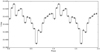 |
Fig. 8 Detrended OGLE light curve folded at the best period, the shape being symmetric and having more of a sinusoidal than a FRED-like profile. |
3.4 Long-term X-ray light curve
Figure 9 shows the long-term X-ray light curve of SXP164 in the time interval covered by the OGLE-IV monitoring (shown again at the bottom). The measured 0.2-12 keV fluxes (dots) and the upper limits (triangles) are derived from both pointed and slew XMM-Newton and Swift observations using the Upper Limit Server (ULS3). The values are derived assuming a power-law spectrum with NH = 1 × 1021 cm−2 and a spectral index Γ = 1, as in Maggi et al. (2013). Chandra observed the source only once, in 2002 August, where the flux was 3.2 × 10⁻¹³ erg cm2 s−1 (Rajoelimanana et al. 2011a). The 0.2–10 keV fluxes from the most recent Swift observations (2019 December 1 to 2020 January 15), which are not included in the ULS, are shown as well and assume the same spectral model (see below). In addition to the pointed observations described in this paper, the source was observed during the eROSITA all-sky surveys eRASS1 (in 2020 April–May), eRASS2 (in 2020 November) and eRASS3 (in 2021 May) with count rates of 0.269 ± 0.044 cts s−1, 0.226 ± 0.043 cts s−1, and 0.546 ± 0.065 cts s−1 (average over successive ~40s scanning observations separated by gaps of ~4h). The count rates are converted into fluxes using the same scaling factor as for the pointed observations. The resulting eROSITA fluxes, as derived in Sect. 3.1.2 and from the surveys, are shown in Fig. 9 in green.
The long-term light curve indicates the possibility that the source became bright simultaneously in the X-ray and the I bands, i.e. from late 2012. Some variability (a factor of -10) is nevertheless present in the high X-ray state. To check if the X-ray variability observed after 2013 could be related to the binary orbit (Type-I outbursts) we analysed two sets of Swift/XRT observations: the first performed from 2013 November 30 (ObsID: 00033042001) to 2014 February 07 (00033042038) with SXP65.8 as target (only with off-axis angles <12’), and the second one running from 2019 December 01 (00012207001) to 2020 January 15 (00012207011), with XMMUJ010429.4–723136 as the target. The 0.3–10 keV vignetting-corrected count rates for these observations were retrieved using the online tool of the UK Swift Science Data Centre4, which is described in Evans et al. (2007) and Evans et al. (2009). The resulting light curve folded at the orbital period (22.35 days) is shown in Fig. 10. These two data sets clearly show large-amplitude modulations that are phase-connected and could be very well explained by the orbital motion. The suggested orbital period is therefore also visible in the X-rays, although a longer monitoring with Swift/XRT would be necessary to increase the significance of the modulation.
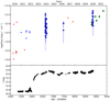 |
Fig. 9 Long-term X-ray light curve of SXP164 (top) during the OGLE monitoring (bottom). Dots represent measured flux, while upper limits are shown as triangles. XMM-Newton (pointed+slew), Swift and eROSITA fluxes are shown in red, blue, and green, respectively. Flux values before 2019 are derived using the ULS. |
 |
Fig. 10 Vignetting-corrected light curve of SXP 164 from two sets of Swift/XRT observations (2013 November to 2014 February in red and 2019 December to 2020 January in blue) folded at the orbital period (22.35 days). |
4 Discussion
We report the discovery of the pulse period (164 s) and possibly the orbital period (22 days) of a known Be/X-ray binary in the SMC. We had a close look at the existing archival X-ray data prior to eROSITA to check whether or not the pulse period could have been detected. In the archival ROSAT and XMM-Newton data, from which the detections are reported by Haberl et al. (2000)5 and in Rosen et al. (2016)6, the source is too faint, while for the Swift observations, the exposures are too short. Only in the unique Chandra observation from 2002 were sufficient photons available, but no period other than that of the spacecraft dithering can be detected.
As for many other Be/X-ray binaries belonging to that galaxy, the source is highly variable in the X-rays with a ratio F max/F min ≳ 750 with Fmax ~ 3.8 x 10⁻¹² and Fmin ≲ 5 × 10⁻¹⁵ erg cm−2 s−1 (upper limit from a XXMM-Newton observation performed in October 2000). Those values are in line with what is reported by Haberl & Sturm (2016) in their Fig. 5 for the other SMC Be/X-ray binaries. Following the analysis of the Swift/XRT observations described in Sect. 3.4, most of the variability could be explained by an orbital modulation at a period of 22 days, which is consistent with the period derived here from the analysis of the OGLE-IV data. We note that Schmidtke et al. (2013) studied the MACHO and OGLE-II data available at the time and find that only a few seasons presented evidence for any periodicity. In OGLE-II data, only the first season shows a prominent period at P = 0.972 days or its alias at 37.1 days. A peak near the 39.7 days period is also visible in our periodogram, but only for the full undetrended light curve.
According to the well-known Corbet diagram (Corbet 1986), an empirical power-law relationship between the pulse period Ps (in seconds) and the orbital period Po (in days) was derived for Be/X-ray binaries based on the observed values, with e being the orbital eccentricity:
 (1)
(1)
A more recent and updated version of this empirical relationship was proposed by Yang et al. (2017) as:
 (2)
(2)
This relationship can be explained for systems being in a state of quasi-equilibrium in which the Alfvén radius (the radius where the inflowing matter couples to the magnetic field lines of the neutron star) and corotation radius (radius where the spin angular velocity of the neutron star is equal to the Keplerian angular velocity) are equal on average. However, on the Corbet diagrams, a large scatter is observed in both papers, as is also shown by Haberl & Sturm (2016), indicating that many systems are probably not in a state of quasi-equilibrium, with their pulse periods still varying. An updated version of the diagram provided by Haberl & Sturm (2016), which includes SXP 164, is shown in Fig. 11. The spin period is somewhat larger with respect to other sources with similar orbital periods, suggesting that the neutron star can still spin-up in the future. SXP 1323 had, for example, a stable pulse period of around 1323 s from 2000 to 2006, and then started to spin-up rapidly from 2006 to 2016 while keeping a constant flux (Carpano et al. 2017), to reach ~1005 s in 2019 November (Haberl et al. 2019) and ~977 s in 2020 October (Haberl et al. 2022).
The comparison of the system's long-term X-ray and OGLE-IV light curves indicates that the flux growth in both wavelength bands is correlated. The long-term optical variations of Be/X-ray binaries are believed to be related to the formation and depletion of the circumstellar disc around the donor star, giving rise to the Be phenomenon, as suggested in Rajoelimanana et al. (2011b). A larger disc could lead to a higher accretion rate onto the neutron star and therefore increase its X-ray luminosity. Since eROSITA is the only instrument that has observed the source in its bright state with a sufficiently long exposure to retrieve the pulse period, new pointed observations would be necessary to explore the long-term impact of a larger Be disc on the pulse period derivative (a possible slow spin-up is suggested from these observations).
The optical spectrum is dominated by the Hα emission line emitted from the circumstellar disc surrounding the Be star and this line is therefore a good probe of the disc. The presence of the Hα emission line is one of the main classification criteria for Be/X-ray binaries. Coe & Kirk (2015); Antoniou et al. (2009) show that a strong correlation exists between the orbital period Porb (d) and the line EW (Å). The linear best fit derived from the EW/Porb distribution of Be/X-ray pulsars in the SMC gives the relationship:
![Mathematical equation: ${{\rm{H}}_\alpha }{\rm{EW({\AA}) = [ - 0}}{\rm{.16}} \times {P_{{\rm{orb}}}}{\rm{(d)] - 9}}{\rm{.7}}$](/articles/aa/full_html/2022/05/aa41082-21/aa41082-21-eq12.png) (3)
(3)
for orbital periods Porb ≤ 150 days (Coe & Kirk 2015, see their Fig. 8). We note that the scatter observed by these latter authors in the EW/Porb distribution is large, especially for the short-period systems, and that it makes use of the largest EW ever measured. The EW/Porb relationship is explained by the disc of the Be star being truncated by the neutron star during its orbit. The neutron star appears to act as a barrier, preventing the formation of an extended disc in systems with short orbital periods. This should also imply that the circumstellar disc, and in turn the Hα EW, are on average smaller in binary systems than for isolated Be stars. Correlations between the spectral parameters of the Hα line and rotational velocity have been observed in many Be stars and are interpreted as evidence for rotationally dominated circumstellar discs (Dachs et al. 1986; Hanuschik et al. 1988; Reig 2011). A monitoring of the Hα EW and profile over a period of a few months could both confirm the 22.3 days orbital period and provide constraints on the inclination angle of the Be disc.
 |
Fig. 11 Spin period vs. orbital period for HMXBs in the SMC, as presented in Haberl & Sturm (2016), including SXP 164. Orbital periods found with different methods are marked with different symbols: full orbit solution (red circles), X-ray outbursts (red squares), optical light curve (green triangles). Blue circles mark systems with orbital periods consistently derived from X-rays and optical. |
Acknowledgements.
This work is based on data from eROSITA, the primary instrument aboard SRG, a joint Russian-German science mission supported by the Russian Space Agency (Roskosmos), in the interests of the Russian Academy of Sciences represented by its Space Research Institute (IKI), and the Deutsches Zentrum für Luft- und Raumfahrt (DLR). The SRG spacecraft was built by Lav-ochkin Association (NPOL) and its subcontractors, and is operated by NPOL with support from the Max Planck Institute for Extraterrestrial Physics (MPE). The development and construction of the eROSITA X-ray instrument was led by MPE, with contributions from the Dr. Karl Remeis Observatory Bamberg & ECAP (FAU Erlangen-Nürnberg), the University of Hamburg Observatory, the Leibniz Institute for Astrophysics Potsdam (AIP), and the Institute for Astronomy and Astrophysics of the University of Tübingen, with the support of DLR and the Max Planck Society. The Argelander Institute for Astronomy of the University of Bonn and the Ludwig Maximilians Universitat Munich also participated in the science preparation for eROSITA. The eROSITA data shown here were processed using the eSASS/NRTA software system developed by the German eROSITA consortium. The optical spectrum presented in this paper were obtained with the Southern African Large Telescope (SALT).
References
- Antoniou, V., Hatzidimitriou, D., Zezas, A., & Reig, P. 2009, ApJ, 707, 1080 [NASA ADS] [CrossRef] [Google Scholar]
- Bird, A. J., Coe, M. J., McBride, V. A., & Udalski, A. 2012, MNRAS, 423, 3663 [NASA ADS] [CrossRef] [Google Scholar]
- Brunner, H., Liu, T., Lamer, G., et al. 2022, A&A, 661, A1 (eROSITA EDR SI) [NASA ADS] [CrossRef] [EDP Sciences] [Google Scholar]
- Buckley, D. A. H., Swart, G. P., & Meiring, J. G. 2006, SPIE Conf. Ser., 6267, 62670Z [Google Scholar]
- Burgh, E. B., Nordsieck, K. H., Kobulnicky, H. A., et al. 2003, SPIE Conf. Ser., 4841, 1463 [NASA ADS] [Google Scholar]
- Carpano, S., Haberl, F., & Sturm, R. 2017, A&A, 602, A81 [NASA ADS] [CrossRef] [EDP Sciences] [Google Scholar]
- Coe, M. J., & Kirk, J. 2015, MNRAS, 452, 969 [NASA ADS] [CrossRef] [Google Scholar]
- Coe, M. J., Edge, W. R. T., Galache, J. L., & McBride, V. A. 2005, MNRAS, 356, 502 [NASA ADS] [CrossRef] [Google Scholar]
- Corbet, R. H. D. 1986, MNRAS, 220, 1047 [NASA ADS] [CrossRef] [Google Scholar]
- Dachs, J., Hanuschik, R., Kaiser, D., et al. 1986, A&AS, 63, 87 [Google Scholar]
- Dickey, J. M., & Lockman, F. J. 1990, ARA&A, 28, 215 [Google Scholar]
- Evans, P. A., Beardmore, A. P., Page, K. L., et al. 2007, A&A, 469, 379 [NASA ADS] [CrossRef] [EDP Sciences] [Google Scholar]
- Evans, P. A., Beardmore, A. P., Page, K. L., et al. 2009, MNRAS, 397, 1177 [Google Scholar]
- Galache, J. L., Corbet, R. H. D., Coe, M. J., et al. 2008, ApJS, 177, 189 [NASA ADS] [CrossRef] [Google Scholar]
- Gotthelf, E. V., Vasisht, G., & Dotani, T. 1999, ApJ, 522, L49 [NASA ADS] [CrossRef] [Google Scholar]
- Haberl, F., & Sturm, R. 2016, A&A, 586, A81 [NASA ADS] [CrossRef] [EDP Sciences] [Google Scholar]
- Haberl, F., Filipović, M. D., Pietsch, W., & Kahabka, P. 2000, A&AS, 142, 41 [NASA ADS] [CrossRef] [EDP Sciences] [Google Scholar]
- Haberl, F., Eger, P., & Pietsch, W. 2008, A&A, 489, 327 [NASA ADS] [CrossRef] [EDP Sciences] [Google Scholar]
- Haberl, F., Carpano, S., Maitra, C., et al. 2019, ATel, 13312, 1 [NASA ADS] [Google Scholar]
- Haberl, F., Maitra, C., Carpano, S., et al. 2022, A&A, 661, A25 (eROSITA EDR SI) [NASA ADS] [CrossRef] [EDP Sciences] [Google Scholar]
- Hanuschik, R. W., Kozok, J. R., & Kaiser, D. 1988, A&A, 189, 147 [NASA ADS] [Google Scholar]
- Hilditch, R. W., Howarth, I. D., & Harries, T.J. 2005, MNRAS, 357, 304 [NASA ADS] [CrossRef] [Google Scholar]
- Lomb, N. R. 1976, Ap&SS, 39, 447 [Google Scholar]
- Maggi, P., Sturm, R., Haberl, F., & Vasilopoulos, G. 2013, ATel, 5674, 1 [NASA ADS] [Google Scholar]
- McBride, V. A., Gonzalez-Galan, A., Bird, A. J., et al. 2017, MNRAS, 467, 1526 [NASA ADS] [CrossRef] [Google Scholar]
- Predehl, P., Andritschke, R., Arefiev, V., et al. 2021, A&A, 647, A1 [EDP Sciences] [Google Scholar]
- Rajoelimanana, A. F., Charles, P.A., & Udalski, A. 2011a, ATel, 3154, 1 [NASA ADS] [Google Scholar]
- Rajoelimanana, A. F., Charles, P.A., & Udalski, A. 2011b, MNRAS, 413, 1600 [NASA ADS] [CrossRef] [Google Scholar]
- Reig, P. 2011, Ap&SS, 332, 1 [Google Scholar]
- Rosen, S. R., Webb, N. A., Watson, M. G., et al. 2016, A&A, 590, A1 [NASA ADS] [CrossRef] [EDP Sciences] [Google Scholar]
- Russell, S. C., & Dopita, M. A. 1992, ApJ, 384, 508 [NASA ADS] [CrossRef] [Google Scholar]
- Scargle, J. D. 1982, ApJ, 263, 835 [Google Scholar]
- Schmidtke, P.C., Cowley, A. P., & Udalski, A. 2013, MNRAS, 431, 252 [NASA ADS] [CrossRef] [Google Scholar]
- Sturm, R., Haberl, F., Pietsch, W., et al. 2013, A&A, 558, A3 [NASA ADS] [CrossRef] [EDP Sciences] [Google Scholar]
- Udalski, A. 2008, Acta Astron., 58, 187 [NASA ADS] [Google Scholar]
- Wilms, J., Allen, A., & McCray, R. 2000, ApJ, 542, 914 [Google Scholar]
- Yang, J., Laycock, S. G. T., Christodoulou, D. M., et al. 2017, ApJ, 839, 119 [NASA ADS] [CrossRef] [Google Scholar]
All Tables
Spectral parameters resulting from the fit to the eROSITA spectra during ObsID 700 001 and 700 003, performed simultaneously, and 710 000, and the corresponding fluxes (absorbed and unabsorbed) and luminosities (in the 0.2–10 keV band and assuming a distance of 60.6 kpc).
All Figures
|
Fig. 1 eROSITA light curve of SXP 164, during ObsID 700 001 (top), 700 003 (middle) and 710 000 (bottom), rebinned at 2000 s, extracted in the 0.2–5.0 keV band. The red lines indicate the mean values of 0.10, 0.12, and 0.16 cts s−1 for the three respective observations. |
| In the text | |
|
Fig. 2 Lomb-Scargle periodogram for the three eROSITA observations (top: ObsID 700 001, middle: 700 003 and bottom: 710 000), using light curves binned at 2 s. The best periods are 163.93 s, 163.85 s, and 163.48 s, respectively. |
| In the text | |
|
Fig. 3 Folded eROSITA light curves of SXP 164 during ObsID 700 001 (top), 700003 (middle), and 710 000 (bottom), extracted in the 0.2–5.0 keV band. The best-fit sine function is overlaid. Phase 0 corresponds to the start of the first observation. The light curves from the first two observations are folded with the common period (163.89 s). |
| In the text | |
|
Fig. 4 Simultaneous spectral fit of SXP 164 using an absorbed power-law model (TBabs*TBvarabs*power), and the corresponding residuals for ObsID 700 001 (3 cameras) and 700 003 (5 cameras) at the top and ObsID 710 000 (5 cameras) at the bottom. |
| In the text | |
|
Fig. 5 Optical spectrum of XMMU J010429.4–723136 obtained on 2019-11-24 using the Robert Stobie Spectrograph on SALT. The rest wavelength of the Hα line is marked. |
| In the text | |
|
Fig. 6 OGLE-IV light curve of SXP 164 in the I band: full light curve (top), detrended (middle), high state only (bottom). |
| In the text | |
|
Fig. 7 Lomb-Scargle periodogram of the OGLE full (top), detrended (middle), and high-state-only (bottom) light curves showing a clear peak at 22.35 days for the detrended and high-state-only light curves (22.09 days in the full light curve). The confidence levels (given at 68%, 90% and 99%) are derived using the block-bootstrap method). |
| In the text | |
|
Fig. 8 Detrended OGLE light curve folded at the best period, the shape being symmetric and having more of a sinusoidal than a FRED-like profile. |
| In the text | |
|
Fig. 9 Long-term X-ray light curve of SXP164 (top) during the OGLE monitoring (bottom). Dots represent measured flux, while upper limits are shown as triangles. XMM-Newton (pointed+slew), Swift and eROSITA fluxes are shown in red, blue, and green, respectively. Flux values before 2019 are derived using the ULS. |
| In the text | |
|
Fig. 10 Vignetting-corrected light curve of SXP 164 from two sets of Swift/XRT observations (2013 November to 2014 February in red and 2019 December to 2020 January in blue) folded at the orbital period (22.35 days). |
| In the text | |
|
Fig. 11 Spin period vs. orbital period for HMXBs in the SMC, as presented in Haberl & Sturm (2016), including SXP 164. Orbital periods found with different methods are marked with different symbols: full orbit solution (red circles), X-ray outbursts (red squares), optical light curve (green triangles). Blue circles mark systems with orbital periods consistently derived from X-rays and optical. |
| In the text | |
Current usage metrics show cumulative count of Article Views (full-text article views including HTML views, PDF and ePub downloads, according to the available data) and Abstracts Views on Vision4Press platform.
Data correspond to usage on the plateform after 2015. The current usage metrics is available 48-96 hours after online publication and is updated daily on week days.
Initial download of the metrics may take a while.