| Issue |
A&A
Volume 661, May 2022
|
|
|---|---|---|
| Article Number | A64 | |
| Number of page(s) | 10 | |
| Section | The Sun and the Heliosphere | |
| DOI | https://doi.org/10.1051/0004-6361/202040006 | |
| Published online | 02 May 2022 | |
Sudden depletion of Alfvénic turbulence in the rarefaction region of corotating solar wind high-speed streams at 1 AU: Possible solar origin?
1
University of L’Aquila, Dept. of Physical and Chemical Sciences, Via Vetoio 48, 67100 Coppito, AQ, Italy
e-mail: This email address is being protected from spambots. You need JavaScript enabled to view it.
2
INAF-Institute for Space Astrophysics and Planetology, Via del Fosso del Cavaliere 100, 00133 Rome, Italy
3
University of Lyon, CNRS, École Centrale de Lyon, INSA de Lyon, Université Claude Bernard Lyon 1, Laboratoire de Mécanique des Fluides et d’Acoustique, UMR5509, 69134 Écully, France
4
University of Michigan, Dept. of Climate and Space Sciences and Engineering, Ann Arbor, MI, USA
Received:
27
November
2020
Accepted:
17
February
2022
Abstract
A canonical description of a corotating solar wind high-speed stream in terms of velocity profile would indicate three main regions: a stream interface or corotating interaction region characterized by a rapid increase in flow speed and by compressive phenomena that are due to dynamical interaction between the fast wind flow and the slower ambient plasma; a fast wind plateau characterized by weak compressive phenomena and large-amplitude fluctuations with a dominant Alfvénic character; and a rarefaction region characterized by a decreasing trend of the flow speed and wind fluctuations that are gradually reduced in amplitude and Alfvénic character, followed by the slow ambient wind. Interesting enough, in some cases, fluctuations are dramatically reduced, and the time window in which the severe reduction of these fluctuations takes place is remarkably short, about some minutes. The region in which the fluctuations are rapidly reduced is located at the flow velocity knee that separates the fast wind plateau from the rarefaction region. The aim of this work is to investigate the physical mechanisms that might be at the origin of this phenomenon. To do this, we searched for any tangential discontinuity that might have inhibited the diffusion of these large-amplitude fluctuations in the rarefaction region as well. We also searched for differences in the composition analysis because minor ions are good tracers of physical conditions in the source regions of the wind under the hypothesis that large differences in the source regions might be linked to the phenomenon observed in situ. We found no positive feedback from these analyses, and finally invoked a mechanism based on interchange reconnection experienced by the field lines at the base of the corona, within the region that separates the open field lines of the coronal hole, which is the source of the fast wind, from the surrounding regions that are mainly characterized by closed field lines. Another possibility clearly is that the observed phenomenon might be due to the turbulent evolution of the fluctuations during the expansion of the wind. However, it is hard to believe that this mechanism would generate a short transition region such as is observed in the phenomenon we discuss. This type of study will greatly benefit from Solar Orbiter observations during the future nominal phase of the mission, when it will be possible to link remote and in-situ data, and from radial alignments between Parker Solar Probe and Solar Orbiter.
Key words: turbulence / Sun: magnetic fields / solar wind / magnetohydrodynamics (MHD) / Sun: corona
© ESO 2022
1. Introduction
The solar wind is an electrically neutral plasma flow that emanates from the basis of the solar corona, permeating and shaping the whole heliosphere. During solar activity minima, when the meridional branches of the polar coronal holes (CHs hereafter) reach the equatorial regions of the Sun, an observer located in the ecliptic plane would record a repeated occurrence of fast (700–800 km s−1) and slow (300–400 km s−1) wind samples. The balance between the two wind classes would change during the evolution of the 11-year solar cycle depending on changes in the topology of the heliomagnetic equator and its inclination on the ecliptic plane. The fast wind originates from unipolar open field line regions, typical of CHs (Schatten & Wilcox 1969; Hassler et al. 1999). The origin of the slow wind is much more uncertain, although we know that this class of wind is generated within regions that are mainly characterized by closed field line configurations that likely inhibit the escape of the wind (Wang & Sheeley 1990; Antonucci et al. 2005; Bavassano et al. 1997; Wu et al. 2000; Hick et al. 1999). The different composition and mass flux of the slow wind and the different degree of elemental fractionation with respect to the corresponding photospheric regions strongly suggest that this slow plasma flow could initially be magnetically trapped and then released (Geiss et al. 1995a,b). The interchange reconnection process plays a fundamental role in opening up the part of the closed field lines that is linked to the convective cells at the photospheric level (Fisk et al. 1999; Fisk & Schwadron 2001; Schwadron 2002; Schwadron et al. 2005; Wu et al. 2000; Fisk & Kasper 2020). This process should preferentially develop close to the border of the CHs and in this way affects the neighboring regions, that is, the coronal hole boundary layer (hereafter CHBL), and the closed-loop corona. During the wind expansion, magnetic field lines from CHs of opposite polarities are stretched into the heliosphere by fast-wind streams that are separated by the heliospheric current sheet (HCS), an ideal plane, magnetically neutral, permeated by slow-wind plasma (Hundhausen 1995). Moreover, because of the solar rotation, the high-speed plasma would overtake and impact any slower plasma ahead of it, creating a compression region (Hundhausen 1972). As a consequence of this interaction, a so-called corotating interaction region (CIR), characterized by a rather rapid increase in the wind speed from values typical of the slow wind (300–400 km s−1) to values typical of the fast wind (700–800 km s−1), forms at the stream-stream interface. The CIR is characterized by strong compressive phenomena (red zone in Fig. 1) that affect the magnetic field and plasma (Richardson 2018).
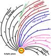 |
Fig. 1. Sketch of a stream structure in the ecliptic plane, adapted from Hundhausen (1972). The spiral structure is a consequence of solar rotation. The spiral inclination changes as the solar wind velocity changes. When the high-speed stream (in blue) compresses the slower ambient solar wind (in black), a compression region downstream (in red) and a rarefaction region upstream (in pink) are formed. The velocity knee marks the border between the blue and pink regions. |
The CIR is followed by a region in which the wind speed persists at its highest values (blue zone in Fig. 1), resembling a sort of plateau, while the other plasma and magnetic field parameters rapidly decrease to remain rather stable across its extension. Beyond this region, highlighted at times by a sharp knee in the radial velocity, the wind speed decreases monotonically to reach values typical of the following slow wind (black zone in Fig. 1), which permeates the interplanetary current sheet. This decreasing wind speed region is slightly more rarefied than the high-speed region that immediately follows the CIR and is commonly called the rarefaction region (pink zone in Fig. 1). For more details about this region, we refer to Borovsky & Denton (2016), who provided a detailed description based on a statistical study. The three regions described above can be considered the imprint in the interplanetary medium of the coronal structure from which the wind originated (Hundhausen 1972). The fast-wind plateau corresponds to the core of the CH, while CIR and rarefaction region correspond to the same CHBL that encircles the CH, although within the CIR, the CHBL is compressed by the dynamical interaction described earlier between fast and slow wind, while within the rarefaction region, the CHBL is stretched by the wind expansion into the interplanetary medium (Schwadron & McComas 2005).
Beyond a few solar radii, the solar wind (both fast and slow) becomes supersonic and super-Alfvénic. Fluctuations in interplanetary magnetic field and plasma parameters show their turbulent character (typical Kolmogorov spectrum) starting from the first few dozen solar radii (Kasper et al. 2019), and in particular, turbulence features within the fast and slow wind differ dramatically (Bruno & Carbone 2013, and references therein). The fast wind is rather uncompressive and mostly characterized by strong Alfvénic correlations between velocity and magnetic field fluctuations, but it also carries compressive fast and slow magnetosonic modes (Marsch & Tu 1990, 1993; Klein et al. 2012; Howes et al. 2012; Verscharen et al. 2019). Alfvénicity in the slow wind is in general much lower and has compressive effects that affect the plasma dynamics more strongly and reflect the complex magnetic and plasma structure of its source regions, close to the heliomagnetic equator (Tu & Marsch 1995; Bruno & Carbone 2013).
This paper studies a peculiar phenomenon that we observe when the s/c crosses the heliospheric current sheet (HCS) with a large pitch angle. In cases like this, large-amplitude Alfvénic fluctuations, populating the fast-wind plateau of a typical high-velocity stream, are abruptly and dramatically depleted in the rarefaction region as soon as the s/c crosses the velocity knee that is located at the border between these two regions of the stream (the blue and pink regions in Fig. 1). As detailed in the following, we realized that while downstream of the knee, plasma and magnetic field fluctuations have large amplitude and are highly Alfvénic, in the upstream region, fluctuations dramatically reduce their amplitude and the Alfvénic correlation weakens and begins to fluctuate between positive and negative values. Interesting enough, the time window of the remarkable depletion of these fluctuations can be very short, a few dozens minutes, and this abrupt reduction is located around the velocity knee, that is, at the end of the fast-wind plateau and at the beginning of the rarefaction region. To our knowledge, no specific analyses have ever been devoted so far to understanding the reason of this sudden and dramatic phenomenon in solar wind turbulence.
2. Data analysis
We selected the whole year 2017, during which solar activity cycle 24 was in its declining phase. We visually inspected about 12 high-velocity streams and found that 3 of them showed turbulence features similar to the phenomenon just described in the introduction. We focused on a corotating high-speed stream for which this phenomenon is particularly noticeable. This stream was observed on 3–9 August 2017, and its velocity profile is shown in Fig. 2, panel a. We also show for comparison another stream observed on 28 February–15 March 2017, in which the reduction in the amplitude of magnetic field and plasma fluctuations and Alfvénicity occurs much more slowly. We compare these two streams to identify the differences in the physical parameters that describe these streams, which might be at the basis of the observed different behavior of turbulence. The analysis was performed using three-second averages of magnetic field and plasma observed at 1AU by the WIND1 spacecraft and two-hour averages of minor ion parameters (highest time resolution available during the selected time intervals) by the ACE2 spacecraft during the last minimum of solar activity. Data are given in heliocentric Earth ecliptic (HEE) reference system, in which the X-axis points along the Sun-Earth line, the Z-axis is perpendicular to the ecliptic plane and points northward, and the Y-axis is oriented such that Z = X × Y concludes the right-handed reference system (Hapgood 1992).
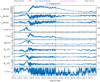 |
Fig. 2. Temporal profiles of solar wind parameters from 3 to 9 August 2017 (215–221 doy), at a time resolution of 6 s. Panels show from top to bottom the proton velocity components in the HEE reference system, Vx (panel a), Vy (panel b), and Vz (panel c), the proton number density (panel d) and proton temperature (panel e), the magnetic field magnitude (panel f) and the magnetic field components in HEE, Bx (panel g), By (panel h), and Bz (panel i), and the angle θ = cos−1(|Bx|/|B|) between the average magnetic field direction and the radial direction (panel j). In the last panel, the dashed black curve represents the local Parker spiral direction, with respect to the high-speed region and rarefaction region. The dashed red line in each panel denotes the velocity knee between the fast-wind region and the rarefaction region. At the top of the figure we indicate the different solar wind regions vertically. The colors correspond to the sketch in Fig. 1. |
The magnetic field and plasma data collected by WIND are not provided with synchronized time stamps. We therefore resampled the time series with a six-second cadence in order to create a single merged data set with a uniform time base that we used to characterize the statistics of the turbulent fluctuations of the solar wind parameters.
2.1. Turbulence analysis
In order to highlight the different character of wind fluctuations within the high-speed plateau and the rarefaction region, we adopted numerical tools typical of turbulence analysis. To characterize the turbulence in the solar wind, we built the Elsässer variables Z± = V ± B (Elsasser 1950), where V is the velocity vector and B is the magnetic field vector expressed in Alfvén units (Tu & Marsch 1995; Bruno & Carbone 2013).
The second-order moments linked to Elsässer variables are (Bruno & Carbone 2013)
 (1a)
(1a)
 (1b)
(1b)
 (1c)
(1c)
 (1d)
(1d)
where δ denotes fluctuations with respect to the mean value of each variable, and angular brackets indicate the averaging process over the established time range. In our case, e±, eV, eB, and ec represent the variances calculated in an hourly moving window for the whole stream. In order to describe the degree of correlation between V and B, it is convenient to use normalized quantities,
 (2a)
(2a)
 (2b)
(2b)
where −1 ≤ σc ≤ 1 and −1 ≤ σr ≤ 1.
The panels of Fig. 2 show some of the plasma and magnetic field features characterizing the particular stream we chose, observed by WIND in August 2017. This is a canonical corotating high-speed stream (Richardson 2018), as described in the introduction, in which an interaction region can easily be recognized. This region occurred at about noon of 4 August (doy 216) and was characterized by a strong magnetic field intensity and plasma number density enhancements, followed by a clear increase in proton temperature (as expected for a compressive region because this stream strongly interacts with the slow wind ahead of it Bruno & Carbone 2013). This interaction region, within which the wind speed rapidly increases from about 400 km s−1 to about 700 km s−1, is followed by a speed plateau that lasts for about two days. The plateau is characterized by fluctuations in velocity and magnetic field components of remarkable amplitude at an hourly scale, ΔV ≃ 28 km s−1 and ΔVA ≃ 42 km s−1 (where  is the Alfvén velocity) and rather constant values of the number density n ∼ 3 cm−3 and field intensity |B|∼5 nT. In addition, the temperature (panel e), although it is lower than that within the preceding interaction region (CIR), is much higher than in the surrounding low-speed regions. The high-speed plateau is then followed by a slowly decreasing wind speed profile that identifies the rarefaction region of this corotating stream. These features are typical for most of the high-speed corotating streams we examined. The abrupt depletion of large-amplitude fluctuations detected in the high-speed plateau across the velocity knee is particular for this stream. The velocity knee is defined with respect to the rapid depletion of the fluctuations of the velocity and magnetic field components, that is, at the end of the fast-wind plateau and at the beginning of the rarefaction region, indicated in Fig. 2 by the vertical dashed red line around day 218 (6 August) at noon. This phenomenon is highlighted by the profile of the curve in panel j, related to the angle θ between the magnetic field vector and the radial direction. The difference in the behavior of this parameter before and after the velocity knee is dramatic, and this transition is rather fast and occurs within minutes. Large angular fluctuations between the magnetic field vector and the radial direction are due to the presence of large-amplitude, uncompressive Alfvénic fluctuations populating the high-speed plateau, which force the tip of the magnetic field vector to move randomly on the surface of a hemisphere that is centered around the background mean field direction (e.g., see Fig. 4 in Bruno et al. 2001). However, immediately after the velocity knee and at the very beginning of the rarefaction region, the amplitude of the fluctuations dramatically decreases, and as a consequence, the angle θ shrinks and its range of variability becomes generally confined between 0° and 45°.
On the other hand, not all streams have the same abrupt depletion of plasma and magnetic field fluctuations after the fast-wind plateau; an example is the stream of March 2017 shown in Fig. 3. We can clearly identify the interaction region, which is characterized by a compression (enhancement of the proton density in panel d), followed by an increase in the magnetic field, proton temperature, and velocity of the solar wind, typical of high-speed corotating streams. Immediately after, there are large fluctuations in velocity and magnetic field components in correspondence to the fast-wind plateau of this stream, which last longer than the previous stream. In this case, unlike the previous one, even though there is a decrease in velocity and magnetic fluctuations in the rarefaction region, this decrease occurs gradually over time (days), therefore in this case, we cannot identify a clear velocity knee. This gradually decreasing trend is also present in the temperature profile (panel e). Moreover, within the rarefaction region, the angular fluctuations between the local field and the radial direction (panel j) change rapidly over time without a clear trend, unlike the August stream. Hence the magnetic field vector fluctuates continuously around the radial direction for almost the entire duration of this second stream.
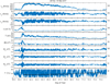 |
Fig. 3. Temporal profiles of solar wind parameters from 28 February to 15 March 2017 (59–74 doy), at a time resolution of 6 s. The panels show the proton velocity components in the HEE reference system, Vx (panel a), Vy (panel b), and Vz (panel c), the proton number density (panel d) and proton temperature (panel e), the magnetic field magnitude (panel f) and magnetic field components in HEE, Bx (panel g), By (panel h), and Bz (panel i), and the angle θ = cos−1(|Bx|/|B|) between the average magnetic field direction and the radial direction (panel j). In the last panel, the dashed black curve represents the local Parker spiral direction with respect to the high-speed region and rarefaction region. |
Comparing the time profiles of the angle θ between the average direction of the magnetic field with respect to the radial direction (panels j of Fig. 2 and Fig. 3), we note that in time correspondence with the fast wind region of both August (Fig. 2j) and March (Fig. 3j) streams, most of the values of θ are above the solid black curve, which indicates the predicted Parker spiral angle based on the wind speed, computed as Ψ = arctan(ΩR/|v|), where R is the distance from the Sun to the Earth, and Ω is the sidereal angular velocity of the Sun at the equator, that is, 2.97 × 10⁻⁶ rad s−1. Consequently, before the velocity knee, the background magnetic field is overwound (Bruno & Bavassano 1997), most likely as a consequence of the dynamical interaction of the fast stream with the slow wind ahead (Schwenn & Marsch 1990). Within the rarefaction region, the time profile of this angle for the March stream rapidly changes, continuously deviating from the local Parker spiral direction. For the August stream, the same angle instead shows a smaller variability with an average direction closer to the radial one and smaller than the local Parker spiral direction, as expected for a rarefaction region (Schwadron & McComas 2005). The existence of this sub-Parker spiral orientation of the background magnetic field depends on the rate of the motion of open magnetic field footpoints across the CHBL at the photospheric level (Schwadron & McComas 2005). This motion is responsible for connecting and stretching magnetic field lines from fast- and slow-wind sources across the CHBL, as explained in the model by Schwadron & McComas (2005). The rarefaction region maps in the interplanetary space the CHBL that encircles the fast-wind source region at the Sun (McComas et al. 2003). The solar wind observed in space and emanating from the CHBL, because of the solar rotation, is characterized by compressive phenomena when detected ahead of the high-velocity stream, and rarefaction phenomena when it is observed following the high-speed plateau.
It is interesting to remark how different the profiles of θ for the two streams are within the rarefaction regions. For the stream of August, the Bx component is generally positive and the profile of θ is largely confined to values below 45°, with sporadic jumps to higher values. For the March stream, the Bx profile is much more structured, and θ continuously fluctuates between 0° and 90°. Moreover, for this last stream, Bx continuously jumps from positive to negative values, suggesting that we must be close to the heliomagnetic equator.
In the upper panel of the left side of Fig. 4 we show the source surface synoptic chart for July–August 2017 taken from the Wilcox Solar Observatory. The purple lines indicate the beginning and the end of the high-speed stream, whose velocity profile is shown in the lower panel. In this case (4–8 August 2017), the heliospheric current sheet is highly inclined with respect to the trajectory of the observer, that is, WIND s/c. On the right side of this figure, we show in the same format as for the left side, the March stream, for which we see no clear and abrupt depletion of the fluctuations. In this case, the velocity profile shows a less clear velocity knee and a slow and progressive depletion of the fluctuations without any abrupt event like the one observed in the previous stream. The main difference, in this case, is that the heliospheric current sheet is very flat and the observer experiences a sort of surfing along this structure, which reflects in a slowly decreasing wind speed because this parameter depends on the angular distance from the interplanetary current sheet (Bruno et al. 1986).
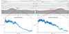 |
Fig. 4. Source surface synoptic charts at 3.25Rs for July–August 2017 on the left side and February–March 2017 on the right side (source: Wilcox Solar Observatory). The level curves indicate values of a constant magnetic field (at 3.25Rs), the black line represents the heliomagnetic equator (current sheet), the two different shades of gray indicate the magnetic field polarity: dark gray and red lines correspond to negative polarity, and light gray and blue lines correspond to positive polarity. The dashed orange line represents the Earth trajectory projected to the solar surface at 3.25Rs. The different purple lines correspond to the periods of the streams. Bottom two panels: velocity profiles of the August 2017 stream (left) and of the March 2017 stream (right). |
As anticipated, the high-speed plateau of the August stream is characterized by large-amplitude Alfvénic fluctuations, as shown in Fig. 5. This figure shows only the fast-wind plateau and the rarefaction region of the stream (216.5–221 doy). The top panel a shows the velocity profile of this corotating high-speed stream. The location of the velocity knee, beyond which large-amplitude magnetic field and plasma fluctuations seem to turn off, is indicated by the vertical dashed red line and determined as follows. Panels b and c show hourly values of kinetic and magnetic energy, respectively, on a semilogarithmic vertical scale. The sharp variation in these two parameters at the end of the speed plateau identifies what we have defined as velocity knee. They remarkably highlight the different physical situation before and after the velocity knee and the abrupt change across it. We note that kinetic energy experiences the strongest decrease, of a factor ∼20. As a consequence, fluctuations within this region become strongly magnetically dominated. In addition, this decrease occurs in correspondence with a strong temperature reduction, as shown in Fig. 2. This strong depletion of proton temperature reflects the thermal pressure decrease (blue trend in Fig. 5 panel i) that starts at the velocity knee. On the other hand, the magnetic pressure (in red) at the velocity knee also increases, so that the wind is maintained in a total pressure (in yellow) balanced status, achieved at the edge of the Alfvénic surface during the initial expansion of the wind (Schwadron & McComas 2005). Figure 5 (panel d) shows the density compressibility over time in a semilogarithmic vertical scale, computed as  , where
  is the variance of the number density at a scale of one hour, and ⟨n⟩ is its average value within the same temporal scale; its value remains quite low (on average 3 × 10⁻³) in the fast-wind region and in the rarefaction region, which is indicative of a fairly incompressible wind, given that the density remains approximately constant in both regions. On the other hand, the compressibility of magnetic field magnitude, computed as
  (Bavassano et al. 1982), where
  is the variance of the magnetic field intensity at a scale of one hour and ⟨|B|⟩ is its average value within the same temporal scale, shown in Fig. 5 (panel e) on a semilogarithmic vertical scale, denotes that magnetic field intensity fluctuations are stronger in correspondence with the fast-wind plateau than in the rarefaction region; there is a sudden reduction at the velocity knee of about an order of magnitude. However, the compressibility of the field intensity is only part of the total power associated with the field fluctuations. As first adopted by Bavassano et al. (1982), the compressibility level of fluctuations at a given timescale is estimated by the ratio of the variance of the field intensity and the total variance of the field, computed as the trace of the covariance matrix at that scale, that is,
  (Bavassano et al. 1982). This parameter can clearly only be ≤1, and its behavior is shown in panel f. Here the magnetic field fluctuations exhibit a lower level of compressibility within the fast-wind plateau, where the Alfvénic nature of turbulence is predominant, and noticeably increases by roughly an order of magnitude, moving across the velocity knee into the rarefaction region. A direct consequence of this increased compressibility is the reduction of the Alfvénicity (Bruno & Bavassano 1991). Panels g and h highlight the Alfvénic nature of these fluctuations within the high-speed plateau. Panel g shows high values of the normalized cross helicity σc, as expected for an Alfvénic wind (Tu & Marsch 1995; Bruno & Carbone 2013) in the fast wind stream. Panel h shows that the normalized residual energy related to the fast wind, although dominated by magnetic energy, is not far from the equipartition expected for Alfvénic fluctuations. Beyond the velocity knee, these two parameters experience a considerable change toward a much lower Alfvénicity, although the transition is not as abrupt as the one relative to the amplitude of these fluctuations, as discussed above.
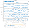 |
Fig. 5. Fast-wind region and rarefaction region of the August 2017 stream. From top to bottom: solar wind speed at a time resolution of 6 s (panel a), values computed in a one-hour moving window of the kinetic energy in semi-logarithmic scale (panel b), magnetic energy in semilogarithmic scale (panel c), density compressibility in semilogarithmic scale (panel d), compressibility of the magnetic field magnitude in semilogarithmic scale (panel e), compressibility of magnetic field fluctuations in semilogarithmic scale (panel f), normalized cross-helicity (panel g), and normalized residual energy (panel h). Bottom panel (panel i) shows an enlargement of the total pressure (yellow), magnetic pressure (orange), and thermal pressure (blue) trend in a small region of a few hours close to the velocity knee. The knee is represented by the dashed red line in each panel. |
The same analysis as in Fig. 5 for the August 2017 stream was also carried out for the fast-wind plateau and rarefaction region of the March 2017 stream (60.75–73 doy) and is shown in Fig. 6. In this case, the decrease in the magnetic field and plasma fluctuations amplitude and Alfvénicity occurs very gradually over time (a few days). The velocity profile (panel a) of the March 2017 stream does not allow us to define a velocity knee in this case. Furthermore, the magnetic energy (panel c) and kinetic energy (panel b) decrease more slowly in the rarefaction region of the stream than in the previous one. The Alfvénic character of the fast wind remains evident, as shown by the profile of σc in panel g and σr in panel h. Even in this case, the density compressibility (panel d) oscillates around very low values of about 10−3, while in this stream, the compressibility of the magnetic field magnitude (panel e) does not show an effective decrease after the velocity plateau, unlike the previous case (August 2017 stream), and the compressibility of magnetic field fluctuations (panel f) undergoes a gradual increase in the transition from the fast-wind plateau to the rarefaction region.
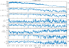 |
Fig. 6. Fast-wind region and rarefaction region of the March 2017 stream. From top to bottom: solar wind speed at a time resolution of 6 s (panel a), values computed in a one-hour moving window of the kinetic energy in semilogarithmic scale (panel b), magnetic energy in semilogarithmic scale (panel c), density compressibility in semilogarithmic scale (panel d), compressibility of the magnetic field magnitude in semilogarithmic scale (panel e), compressibility of magnetic field fluctuations in semilogarithmic scale (panel f), normalized cross-helicity (panel g), and normalized residual energy (panel h). The downward spike in correspondence of doy 65 is an edge effect due to the gap of about 2 h. |
The strikingly different turbulence behavior along the speed profile of these two streams led us to search for a sort of barrier, such as a tangential discontinuity (TD hereafter), located between the end of the fast-wind plateau and the beginning of the rarefaction region, which might have inhibited Alfvénic fluctuations to fill up the rarefaction region of the August 2017 stream. The presence of a TD, where by definition there is no magnetic component normal to the discontinuity surface, could explain the depletion of Alfvén waves (Hundhausen 1972). These fluctuations would not propagate across this type of discontinuity because the magnetic component perpendicular to the discontinuity plane vanishes. This would prevent their propagation into the CHBL or rarefaction region and would produce the observed sudden depletion of the Alfvénic fluctuations. However, we did not find any relevant TD that might be associated with the observed phenomenon. Thus TD cannot be a valid explanation of the rapid decrease in Alfvénic fluctuations at the velocity knee; therefore we searched for a different explanation for this phenomenon that could be due to a different evolution of the solar wind during its expansion or some mechanism acting at the source region of the observed wind. This last possibility is analyzed in the next section.
2.2. Composition analysis
The possibility to link the solar wind to its solar sources is offered by composition analysis of the wind because its parameters, such as ionic and elemental composition, are set within the first few solar radii and do not change during the expansion (Zurbuchen et al. 2002; Bochsler 2007; Landi et al. 2012). Moreover, different sources of the solar wind, for instance, open field line regions versus closed field line regions, exhibit different elemental abundance (Zurbuchen et al. 1999, 2002; von Steiger et al. 2001) and are a valid tool for studying transition regions between the fast coronal wind and the slow wind. Minor ion parameters such as freezing-in temperature and relevance of low first ionization potential (low-FIP) elements (Geiss et al. 1995a,b; McComas et al. 2003) monotonically increase from the fast to the slow wind. Geiss et al. (1995a) and Phillips et al. (1995), based on Ulysses observations, found several dramatic differences in ion composition between the fast and slow wind. One of the most relevant differences is the strong bias of the slow wind in favor of low-FIP elements with respect to the fast wind. Geiss et al. (1995b) used charge-state ratios for C6+/C5+ and O7+/O6+ to estimate the corresponding freezing-in temperatures for these elements and found that slow-wind sources at the Sun are quite hotter than fast wind sources. Finally, fast and slow wind greatly differ also for the higher abundance of He++ within the fast and hot wind with respect to the slow and cold wind (Kasper et al. 2012). Thus, if the rarefaction region were a type of wind that were largely mixed with the slower wind, it would be highlighted by the composition analysis. Consequently, we searched for possible signatures in elemental abundance and charge state, assuming the rapid depletion of magnetic field and plasma fluctuations and Alfvénicity might have a counterpart in composition differences at the source regions.
The four panels of Fig. 7 show from top to bottom the relative abundance of He++/p+ (panel a), some charge-state ratios for carbon and oxygen (panel b), the charge state for iron (panel c), and the relative abundance of iron to oxygen (panel d). Figure 7 refers to the entire stream, that is, the compressive region followed by the high-speed plateau, followed by the rarefaction region, and finally, followed by the slow wind (for comparison, see Fig. 2). The top panel shows the He++/p+ ratio, and although higher values for this parameter are found within the high-speed plateau, the transition across the velocity knee is quite smooth. Moreover, the last three panels of Fig. 7 show a gradual increase from the fast-wind plateau to the rarefaction region, but without a sharp jump across the velocity knee. In particular, the charge-state ratio profile of C6+/C5+ (see the blue curve in panel b of Fig. 7) agrees with the results shown by Schwadron et al. (2005). They modeled a solar minimum configuration that gives rise to a corotating region considering the differential motion of magnetic field foot points at the Sun across the CHBL. In their model, they started the simulation at 30Rs (∼0.14 AU) with a discontinuity at the stream interface (which comes before the fast wind plateau) and another discontinuity at the CHBL. They showed that the discontinuity at the stream interface remains, whereas the discontinuity at the CHBL in the rarefaction region is eroded as the distance from the Sun increases (they extended the simulation to 5 AU). This is exactly what we observe in the carbon charge ratio (panel b of Fig. 7): a rapid decrease at the stream interface, corresponding to a CH discontinuity before the fast-wind plateau, and more importantly, a gradual increase in C6+/C5+ in the rarefaction region, corresponding to the CHBL described in the model of Schwadron et al. (2005). Very similar results were obtained for the March stream, as shown in Fig. 8.
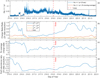 |
Fig. 7. Temporal profiles of ion compositions during the August 2017 stream. Panel a: alpha particle to proton ratio He++/p+ at a time resolution of 6 s (in blue) and its hourly moving average (in red). Panel b: charge-state ratio at a time resolution of 2 h of C6+/C5+ in blue, O7+/O6+ in red, and O8+/O6+ in yellow. Panel c: iron average charge state at a time resolution of 2 h. Panel d: iron to oxygen abundance ratio at a time resolution of 2 h. The dashed red line denotes the velocity knee between the fast-wind region and the rarefaction region. |
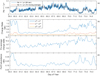 |
Fig. 8. Temporal profiles of ion compositions during the March 2017 stream. Panel a: alpha particle to proton ratio He++/p+ at a time resolution of 64 s (in blue) and its hourly moving average (in red). Panel b: charge-state ratio at a time resolution of 2 h of C6+/C5+ in blue, O7+/O6+ in red and O8+/O6+ in yellow. Panel c: iron average charge state at a time resolution of 2 h. Panel d: iron to oxygen abundance ratio at a time resolution of 2 h. |
Thus, from the composition analysis, we can conclude that there are neither relevant jumps in composition parameters in correspondence to the end of the fast-wind plateau nor large differences between the two streams of August and March to justify a possible link to the abrupt changes in the fluctuations we observe for the August stream. Therefore, these similarities strongly suggest that the reason for the sudden depletion of turbulence observed within the stream of August 2017 and not observed within the stream of March 2017 cannot be linked to relevant different plasma conditions in the source region at the photospheric level.
2.3. Possible role of interchange reconnection
The analysis described in the previous sections neither supports the presence of a TD, which would represent an obstacle for the Alfvénic fluctuations to fill up the rarefaction region, nor the evidence for relevant features in the minor ion composition analysis, which might indicate abrupt changes in the source region of interest. Thus, if this is not the case, we are left with the option that the sudden depletion of turbulence at the velocity knee originates in the source region of the wind, and we suggest that interchange reconnection processes might play a fundamental role in it. As already discussed in the introduction, interchange reconnection between open and closed field lines plays a major role in the regions bordering the CH (Fisk et al. 1999; Fisk & Schwadron 2001; Fisk 2005; Fisk & Kasper 2020; Schwadron et al. 2005). This mechanism governs the diffusion of open magnetic flux outside the CH. The motion of the footpoints of the magnetic field lines due to photospheric dynamics is at the basis of interchange reconnection, which tends to mix open field line regions with nearby closed-loop regions. Alfvénic fluctuations mainly propagate along magnetic field lines, and although these fluctuations are expected to be omnipresent at the photospheric level (Title et al. 1998), they would experience a different fate in open or closed magnetic structures because in the latter, counter-propagating Alfvénic modes would ignite turbulence process, with the consequent transfer of energy to increasingly smaller scales to eventually dissipate and heat the plasma. Thus, we would expect a smaller amplitude and weaker Alfvénic character in these fluctuations coming from originally closed field regions, and a larger amplitude and stronger Alfvénic character for those coming from open field line regions. Based on the interchange reconnection mechanism, an open field line region populated by propagating Alfvénic fluctuations might reconnect with a nearby closed-loop region, as shown in Fig. 9. The left panel A of Fig. 9 sketches open magnetic field lines rooted inside a CH, and coronal loops rooted inside a CHBL, encircling the CH. Large-amplitude Alfvénic fluctuations populate open field lines inside the CH, while fluctuations much reduced in amplitude propagate along the closed field lines in the surrounding regions. A reconnection event like the one sketched in the right panel B of Fig. 9 would cause a sudden depletion of these large-amplitude Alfvénic fluctuations from part of the original open field lines, possibly similar to what we observe in space.
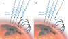 |
Fig. 9. Proposed mechanism of interchange reconnection invoked to explain the abrupt depletion of Alfvénic fluctuations often observed in corotating high-velocity streams. More details in the text. |
3. Summary
Corotating high-speed streams are generally characterized by a high-speed plateau followed by a slow velocity decrease, commonly identified as the stream rarefaction region. These two portions of the stream are in some cases separated by a clear velocity knee. In these cases, the knee also indicates the point beyond which Alfvénic fluctuations, which generally populate the high-speed plateau, are dramatically and rapidly depleted. Interesting enough, this thin border region is not characterized by either any relevant magnetic field structure, for example, a TD, which might cause this abrupt depletion of the fluctuations, or relevant clues in the composition analysis, which might support a different origin in the source region between the wind observed in the high-speed plateau and that observed in the rarefaction region. We cannot exclude that this situation might develop during wind expansion. MHD simulations of an ensemble of Alfvénic fluctuations propagating in an expanding solar wind including the presence of fast and slow solar wind streams reported by Shi et al. (2020) showed that the decrease in σc is more significant in the compression and rarefaction regions of the stream than within the fast and slow streams. In particular, in the rarefaction region of these simulations, σc rapidly decreases from 1 to 0.6 at R ≈ 80Rs and remains at about this value until the end of the simulation. However, it remains to be proven that turbulence evolution would be able to produce abrupt changes in the amplitude and Alfvénicity of the fluctuations such as those we have observed in streams similar to the one of August 2017. The short timescales at which this abrupt decrease in the amplitude of magnetic field and plasma fluctuations (few minutes) and Alfvénicity (less than one hour) is observed make us lean towards the hypothesis that a magnetic reconnection event during the initial phase of the wind expansion might be the mechanism responsible for what we observed and described in this paper. Phenomena of interchange magnetic reconnection favored by the motion of the footpoints of magnetic field lines due to photospheric dynamics would mix field lines that originate from open field line regions, which are robustly populated by large-amplitude Alfvénic fluctuations, with magnetic loops, which are characteristic of surrounding closed field line regions, which are populated by smaller amplitude and less Alfvénic fluctuations. This suggested mechanism, which we cannot prove but propose as a hypothesis at present, could be tested in the near future as soon as the nominal phase of the Solar Orbiter mission will start and it will become possible to directly link in-situ and remote observations. Moreover, this particular kind of study would also greatly benefit from a future radial alignment between Parker Solar Probe and Solar Orbiter, which might allow us to observe wind turbulence for case studies such as the August 2017 stream at different radial distances.
There is no doubt that the single-case study reported in this paper is interesting per se and deserves to be understood. It is greatly stimulating to observe such a quick and remarkable reduction of the turbulence strength in magnetic and kinetic fluctuations without finding any clear reason in the available observations. Even if this were the only case observed so far in the solar wind, it would be wise to study it. In reality, as we already stated, we observed several other streams with the same features, but this is not a statistical study, and we limited our analysis to the August 2017 stream. No similar studies are available in the literature, and our work represents the first attempt in this direction.
Wind 3D Plasma Analyzer and Wind Magnetic Fields Investigation.
ACE/SWICS 2.0 Solar Wind 2 and K0 – ACE Solar Wind Experiment.
Acknowledgments
This work was partially supported by the Italian Space Agency (ASI) under contract ACCORDO ATTUATIVO n. 2018-30-HH.O. Results from the data analysis presented in this paper are directly available from the authors. WIND data have been accessed through the NASA SPDF-Coordinated Data Analysis Web. G.C. acknowledges support from Univ Lyon, CNRS, École Centrale de Lyon, INSA Lyon, Univ Claude Bernard Lyon 1, Laboratoire de Mécanique des Fluides et d’Acoustique, UMR5509, 69134 Écully, France. G.C. acknowledges SWICo’s recognition through the award “Premio Mariani” 2021. R.M. acknowledges support from the project “EVENTFUL” (ANR-20-CE30-0011), funded by the ANR program AAPG-2020.
References
- Antonucci, E., Abbo, L., & Dodero, M. A. 2005, A&A, 435, 699 [NASA ADS] [CrossRef] [EDP Sciences] [Google Scholar]
- Bavassano, B., Dobrowolny, M., Fanfoni, G., Mariani, F., & Ness, N. F. 1982, Sol. Phys., 78, 373 [CrossRef] [Google Scholar]
- Bavassano, B., Woo, R., & Bruno, R. 1997, Geophys. Res. Lett., 24, 1655 [NASA ADS] [CrossRef] [Google Scholar]
- Bochsler, P. 2007, A&ARv, 14, 40 [NASA ADS] [CrossRef] [Google Scholar]
- Borovsky, J. E., & Denton, M. H. 2016, J. Geophys. Res. Space Phys., 121, 6107 [NASA ADS] [CrossRef] [Google Scholar]
- Bruno, R., & Bavassano, B. 1991, J. Geophys. Res. Space Phys., 96(A5), 7841 [NASA ADS] [CrossRef] [Google Scholar]
- Bruno, R., & Bavassano, B. 1997, Geophys. Res. Lett., 24, 2267 [NASA ADS] [CrossRef] [Google Scholar]
- Bruno, R., & Carbone, V. 2013, Liv. Rev. Sol. Phys., 10, 208 [NASA ADS] [Google Scholar]
- Bruno, R., Villante, U., Bavassano, B., Schwenn, R., & Mariani, F. 1986, Sol. Phys., 104, 431 [NASA ADS] [CrossRef] [Google Scholar]
- Bruno, R., Carbone, V., Veltri, P., Pietropaolo, E., & Bavassano, B. 2001, Planet. Space Sci., 49(12), 1201 [Google Scholar]
- Cranmer, Steven R. 2018, ApJ, 862, 1 [NASA ADS] [CrossRef] [Google Scholar]
- D’Amicis, R., & Bruno, R. 2015, ApJ, 805, 9 [CrossRef] [Google Scholar]
- Elsasser, W. M. 1950, Phys. Rev., 79, 183 [Google Scholar]
- Fisk, L. A. 2005, ApJ, 626, 563 [Google Scholar]
- Fisk, L. A., & Kasper, J. C. 2020, ApJ, 894, 5 [Google Scholar]
- Fisk, L. A., & Schwadron, N. A. 2001, ApJ, 560, 425 [Google Scholar]
- Fisk, L. A., Zurbuchen, T. H., & Schwadron, N. A. 1999, ApJ, 521, 868 [Google Scholar]
- Geiss, J., von Gloeckler, G., & Steiger, R. 1995a, Science, 268, 1033 [CrossRef] [Google Scholar]
- Geiss, J., Gloeckler, G., von Steiger, R., et al. 1995b, Space Sci. Rev., 72, 49 [NASA ADS] [CrossRef] [Google Scholar]
- Hapgood, M. A. 1992, Planet. Space Sci., 40, 711 [Google Scholar]
- Hassler, D. M., Dammasch, I. E., Lemaire, P., et al. 1999, Science, 283, 810 [Google Scholar]
- Hick, P., Svestka, Z., Jackson, B. V., Farnik, F., & Hudson, H. 1999, Sol. Wind Nine, 471, 231 [NASA ADS] [CrossRef] [Google Scholar]
- Hollweg, J. V. 2006, Phil. Trans. R. Soc. London Ser. A, 364, 505 [Google Scholar]
- Howes, G. G., Bale, S. D., Klein, K. G., et al. 2012, ApJ, 753, 1 [CrossRef] [Google Scholar]
- Hundhausen, A. J. 1972, Coronal Expansion and Solar Wind (Berlin: Springer-Verlag), 5 [CrossRef] [Google Scholar]
- Hundhausen, A. J. 1995, The Solar Wind, Introduction to Space Physics, eds. M. G. Kivelson, & C. T. Russell, (Cambridge: Cambridge University Press), 91 [CrossRef] [Google Scholar]
- Kasper, J. C., Stevens, M. L., Korreck, K. E., et al. 2012, ApJ, 745, 162 [Google Scholar]
- Kasper, J. C., Bale, S. D., Belcher, J. W., et al. 2019, Nature, 576, 228 [Google Scholar]
- Kigure, H., Takahashi, K., Shibata, K., Yokoyama, T., & Nozawa, S. 2010, PASJ, 62, 993 [Google Scholar]
- Klein, K. G., Howes, G. G., TenBarge, J. M., et al. 2012, ApJ, 755, 2 [NASA ADS] [CrossRef] [Google Scholar]
- Landi, E., Gruesbeck, J. R., Lepri, S. T., Zurbuchen, T. H., & Fisk, L. A. 2012, ApJ, 761, 48 [NASA ADS] [CrossRef] [Google Scholar]
- Lazarian, A., Eyink, G., Vishniac, E., & Kowal, G. 2015, Phil. Trans. R. Soc. London Ser. A, 373, 20140144 [Google Scholar]
- Malara, F., Primavera, L., & Veltri, P. 1996, J. Geophys. Res.: Space Phys., 101, 21617 [Google Scholar]
- Marsch, E., & Tu, C. Y. 1993, Ann. Geophys., 11, 659 [Google Scholar]
- Marsch, E., & Tu, C.-Y. 1990, J. Geophys. Res., 95, 11945 [NASA ADS] [CrossRef] [Google Scholar]
- McComas, D. J., Riley, P., Gosling, J. T., Balogh, A., & Forsyth, R. 1998, J. Geophys. Res., 103, 1955 [NASA ADS] [CrossRef] [Google Scholar]
- McComas, D. J., Elliott, H. A., Schwadron, N. A., et al. 2003, Geophys. Res. Lett., 30, 1517 [Google Scholar]
- Parker, E. N. 1957, J. Geophys. Res., 62, 509 [Google Scholar]
- Phillips, K. J. H., Pike, C. D., Lang, J., et al. 1995, AdSpR, 15, 33 [NASA ADS] [Google Scholar]
- Richardson, I. G. 2018, Liv. Rev. Sol. Phys., 15, 1 [Google Scholar]
- Schatten, K. H., & Wilcox, J. M. 1969, Bull. Am. Astron. Soc. [Google Scholar]
- Schwadron, N. A. 2002, Geophys. Res. Lett., 29, 1663 [NASA ADS] [Google Scholar]
- Schwadron, N. A., & McComas, D. J. 2005, Geophys. Res. Lett., 32 [CrossRef] [Google Scholar]
- Schwadron, N. A., McComas, D. J., Elliott, H. A., et al. 2005, J. Geophys. Res. (Space Phys.), 110, A04104 [NASA ADS] [CrossRef] [Google Scholar]
- Schwenn, R., & Marsch, E. 1990, Physics of the Inner Heliosphere. 1. Large-scale Phenomena (Physics and Chemistry in Space), 20 [CrossRef] [Google Scholar]
- Shi, C., Velli, M., Tenerani, A., & Réville, V. 2020, ApJ, 888, 15 [NASA ADS] [CrossRef] [Google Scholar]
- Shi, C., Velli, M., Panasenco, O., et al. 2021, A&ARv, 650, 12 [Google Scholar]
- Title, A. M., & Schrijver, C. J. 1998, in 10th Cambridge Workshop on Cool Stars, Stellar Systems and the Sun, eds. R. Donahue, & J. Bookbinder (ASP: San Francisco, CA), ASP Conf. Proc., 154, 345 [Google Scholar]
- Tu, C.-Y., & Marsch, E. 1994, J. Geophys. Res., 99(21), 481 [NASA ADS] [CrossRef] [Google Scholar]
- Tu, C.-Y., & Marsch, E. 1995, Space Sci. Rev., 73, 1 [Google Scholar]
- Verscharen, D., Klein, G. K., & Maruca, B. A. 2019, Liv. Rev. Sol. Phys., 16, 5 [NASA ADS] [CrossRef] [Google Scholar]
- von Steiger, R., Zurbuchen, T., Geiss, J., et al. 2001, Space Sci. Rev., 97, 123 [NASA ADS] [CrossRef] [Google Scholar]
- Wang, Y.-M., & Sheeley, N. R. 1990, ApJ, 355, 726 [NASA ADS] [CrossRef] [Google Scholar]
- Wang, Y.-M., & Sheeley, N. R. 2006, ApJ, 653, 708 [NASA ADS] [CrossRef] [Google Scholar]
- Wu, S. T., Wang, A. H., Plunkett, S. P., & Michels, D. J. 2000, ApJ, 545, 1101 [NASA ADS] [CrossRef] [Google Scholar]
- Zurbuchen, T. H., Hefti, S., Fisk, L. A., Gloeckler, G., & von Steiger, R. 1999, The Transition Between Fast and Slow Solar Wind from Composition Data, Coronal Holes and Solar Wind Acceleration, eds. J. L. Kohl, & S. R. Cranmer (Dordrecht: Springer) [Google Scholar]
- Zurbuchen, T. H., Fisk, L. A., von Gloeckler, G., & Steiger, R. 2002, Geophys. Res. Lett., 29, 66 [Google Scholar]
All Figures
|
Fig. 1. Sketch of a stream structure in the ecliptic plane, adapted from Hundhausen (1972). The spiral structure is a consequence of solar rotation. The spiral inclination changes as the solar wind velocity changes. When the high-speed stream (in blue) compresses the slower ambient solar wind (in black), a compression region downstream (in red) and a rarefaction region upstream (in pink) are formed. The velocity knee marks the border between the blue and pink regions. |
| In the text | |
|
Fig. 2. Temporal profiles of solar wind parameters from 3 to 9 August 2017 (215–221 doy), at a time resolution of 6 s. Panels show from top to bottom the proton velocity components in the HEE reference system, Vx (panel a), Vy (panel b), and Vz (panel c), the proton number density (panel d) and proton temperature (panel e), the magnetic field magnitude (panel f) and the magnetic field components in HEE, Bx (panel g), By (panel h), and Bz (panel i), and the angle θ = cos−1(|Bx|/|B|) between the average magnetic field direction and the radial direction (panel j). In the last panel, the dashed black curve represents the local Parker spiral direction, with respect to the high-speed region and rarefaction region. The dashed red line in each panel denotes the velocity knee between the fast-wind region and the rarefaction region. At the top of the figure we indicate the different solar wind regions vertically. The colors correspond to the sketch in Fig. 1. |
| In the text | |
|
Fig. 3. Temporal profiles of solar wind parameters from 28 February to 15 March 2017 (59–74 doy), at a time resolution of 6 s. The panels show the proton velocity components in the HEE reference system, Vx (panel a), Vy (panel b), and Vz (panel c), the proton number density (panel d) and proton temperature (panel e), the magnetic field magnitude (panel f) and magnetic field components in HEE, Bx (panel g), By (panel h), and Bz (panel i), and the angle θ = cos−1(|Bx|/|B|) between the average magnetic field direction and the radial direction (panel j). In the last panel, the dashed black curve represents the local Parker spiral direction with respect to the high-speed region and rarefaction region. |
| In the text | |
|
Fig. 4. Source surface synoptic charts at 3.25Rs for July–August 2017 on the left side and February–March 2017 on the right side (source: Wilcox Solar Observatory). The level curves indicate values of a constant magnetic field (at 3.25Rs), the black line represents the heliomagnetic equator (current sheet), the two different shades of gray indicate the magnetic field polarity: dark gray and red lines correspond to negative polarity, and light gray and blue lines correspond to positive polarity. The dashed orange line represents the Earth trajectory projected to the solar surface at 3.25Rs. The different purple lines correspond to the periods of the streams. Bottom two panels: velocity profiles of the August 2017 stream (left) and of the March 2017 stream (right). |
| In the text | |
|
Fig. 5. Fast-wind region and rarefaction region of the August 2017 stream. From top to bottom: solar wind speed at a time resolution of 6 s (panel a), values computed in a one-hour moving window of the kinetic energy in semi-logarithmic scale (panel b), magnetic energy in semilogarithmic scale (panel c), density compressibility in semilogarithmic scale (panel d), compressibility of the magnetic field magnitude in semilogarithmic scale (panel e), compressibility of magnetic field fluctuations in semilogarithmic scale (panel f), normalized cross-helicity (panel g), and normalized residual energy (panel h). Bottom panel (panel i) shows an enlargement of the total pressure (yellow), magnetic pressure (orange), and thermal pressure (blue) trend in a small region of a few hours close to the velocity knee. The knee is represented by the dashed red line in each panel. |
| In the text | |
|
Fig. 6. Fast-wind region and rarefaction region of the March 2017 stream. From top to bottom: solar wind speed at a time resolution of 6 s (panel a), values computed in a one-hour moving window of the kinetic energy in semilogarithmic scale (panel b), magnetic energy in semilogarithmic scale (panel c), density compressibility in semilogarithmic scale (panel d), compressibility of the magnetic field magnitude in semilogarithmic scale (panel e), compressibility of magnetic field fluctuations in semilogarithmic scale (panel f), normalized cross-helicity (panel g), and normalized residual energy (panel h). The downward spike in correspondence of doy 65 is an edge effect due to the gap of about 2 h. |
| In the text | |
|
Fig. 7. Temporal profiles of ion compositions during the August 2017 stream. Panel a: alpha particle to proton ratio He++/p+ at a time resolution of 6 s (in blue) and its hourly moving average (in red). Panel b: charge-state ratio at a time resolution of 2 h of C6+/C5+ in blue, O7+/O6+ in red, and O8+/O6+ in yellow. Panel c: iron average charge state at a time resolution of 2 h. Panel d: iron to oxygen abundance ratio at a time resolution of 2 h. The dashed red line denotes the velocity knee between the fast-wind region and the rarefaction region. |
| In the text | |
|
Fig. 8. Temporal profiles of ion compositions during the March 2017 stream. Panel a: alpha particle to proton ratio He++/p+ at a time resolution of 64 s (in blue) and its hourly moving average (in red). Panel b: charge-state ratio at a time resolution of 2 h of C6+/C5+ in blue, O7+/O6+ in red and O8+/O6+ in yellow. Panel c: iron average charge state at a time resolution of 2 h. Panel d: iron to oxygen abundance ratio at a time resolution of 2 h. |
| In the text | |
|
Fig. 9. Proposed mechanism of interchange reconnection invoked to explain the abrupt depletion of Alfvénic fluctuations often observed in corotating high-velocity streams. More details in the text. |
| In the text | |
Current usage metrics show cumulative count of Article Views (full-text article views including HTML views, PDF and ePub downloads, according to the available data) and Abstracts Views on Vision4Press platform.
Data correspond to usage on the plateform after 2015. The current usage metrics is available 48-96 hours after online publication and is updated daily on week days.
Initial download of the metrics may take a while.