| Issue |
A&A
Volume 660, April 2022
|
|
|---|---|---|
| Article Number | L4 | |
| Number of page(s) | 6 | |
| Section | Letters to the Editor | |
| DOI | https://doi.org/10.1051/0004-6361/202243361 | |
| Published online | 05 April 2022 | |
Letter to the Editor
Cloud-cloud collision as origin of the G31.41+0.31 massive protocluster
1
INAF-Osservatorio Astrofisico di Arcetri, Largo E. Fermi 5, 50125 Firenze, Italy
e-mail: This email address is being protected from spambots. You need JavaScript enabled to view it.
2
Centro de Astrobiología (CSIC-INTA), Ctra. de Ajalvir Km. 4, Torrejón de Ardoz, 28850 Madrid, Spain
3
Instituto de Astrofísica e Ciências do Espaço, Universidade do Porto, CAUP, Rua das Estrelas, 4150-762 Porto, Portugal
Received:
18
February
2022
Accepted:
18
March
2022
Abstract
The G31.41+0.31 (G31) hot molecular core (HMC) is a high-mass protocluster showing accelerated infall and rotational spin-up that is well studied at high-angular resolution. To complement the accurate view of the small scale in G31, we traced the kinematics of the large-scale material by carrying out N2H+ (1–0) observations with the Institute de Radioastronomie Millimétrique 30m telescope of an area of ∼6 × 6 arcmin2 around the HMC. The N2H+ observations have revealed a large-scale (5 pc) hub-filament system (HFS) composed of at least four filamentary arms and a NNE–SSW velocity gradient (∼0.4 km s−1 pc−1) between the northern and southern filaments. The linewidth increases toward the hub at the center of the HFS reaching values of 2.5–3 km s−1 in the central 1 pc. The origin of the large-scale velocity gradient is likely a cloud-cloud collision. In this scenario, the filaments in G31 would have formed by compression resulting from the collision, and the rotation of the HMC observed at scales of 1000 au would have been induced by shear caused by the cloud-cloud collision at scales of a few parsecs. We conclude that G31 represents a HFS in a compressed layer with an orthogonal orientation to the plane of the sky, and it represents a benchmark for the filaments-to-clusters paradigm of star formation.
Key words: ISM: individual objects: G31.41+0.31 / stars: formation / stars: massive
© ESO 2022
1. Introduction
G31.41+0.31 (G31 hereafter) is a high-mass star-forming region located at 3.75 kpc (Immer et al. 2019) and with a luminosity of ∼5 × 10⁴ L⊙ which harbors a very chemically rich hot molecular core (HMC; e.g., Beltrán et al. 2009; Rivilla et al. 2017; Mininni et al. 2020; Colzi et al. 2021) and an ultra-compact (UC) HII region, located at ∼5″ from the HMC. The region has been extensively observed at high-angular resolution (< 1″) with interferometers, and the observations have revealed the following. First, the HMC has already fragmented and formed a small protocluster composed of at least four massive sources within 1″ (Beltrán et al. 2021). In addition to the sources embedded in the Main core of G31, there are six additional millimeter sources in the region, very close to the HMC and located in what appears to be streams or filaments of matter pointing to the HMC (Beltrán et al. 2021). Second, the core displays a clear NE–SW velocity gradient, observed in several high-density tracers, that has been interpreted to be due to rotation (Beltrán et al. 2004, 2005, 2018; Girart et al. 2009; Cesaroni et al. 2011). Third, the core is still actively accreting, and the kinematics studied at high-angular resolution (∼0 or 750 au) indicates accelerating infall and rotational spin-up (Beltrán et al. 2018). Fourth, dust polarization observations reveal an hourglass-shaped magnetic field with the symmetry axis oriented perpendicular to the velocity gradient (Girart et al. 2009; Beltrán et al. 2019).
The wide-field infrared (IR) view of the G31 region as observed with Spitzer at 8 μm provides evidence that this well-studied (at small scales) HMC is located at the junction of multiple filaments (Fig. 1). This, together with the existence of a protocluster of millimeter sources in G31 (Beltrán et al. 2021), suggests that this massive core might represent the young protostellar hub of a large hub-filament system (HFS), similar to those described by the Filaments to Clusters (F2C) scheme of Kumar et al. (2020). This paradigm proposes the following four stages for massive star formation (see Fig. 14 of Kumar et al. 2020). First, dense filaments, which formed via mechanisms such as cloud–cloud collision, move toward each other and set up the initial conditions for the formation of a HFS. Second, filaments collide and form a hub. The hub gains a twist as the overlap point is different from the center of mass and this gives rise to an initial angular momentum. The resulting spin can eventually flatten the hub. Third, column density amplification in the hub triggers star formation and produces a gravitational potential difference between the hub and the filament, which can drive longitudinal flows within the filaments directed toward the hub. Fourth, radiation pressure and ionization feedback from the newly formed OB stars escapes through the interfilamentary cavities by punching holes in the flattened hub. The filaments are eroded by the expanding radiation bubbles creating pillars, while a mass-segregated embedded cluster is formed in the hub.
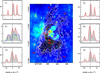 |
Fig. 1. Total N2H+ (1–0) emission integrated between 80 and 110 km s−1 overlaid on the wide-field IR Spitzer 8 μm image of the G31 star-forming region (middle panel). The coordinates are J2000 right ascension and declination. The white contours show emission levels from 0.5 to 3 K km s−1 (in steps of 0.5 K km s−1), and from 4 to 24 K km s−1 (in steps of 2 K km s−1). The red dots and the red dashed areas denote selected positions and regions, respectively, whose spectra are shown in the left and right panels. Left and right panels: N2H+ (1–0) spectra (gray histograms) toward selected positions and regions. The red curves show the best LTE fit obtained with MADCUBA. Blue and green curves in P1 show the two velocity components that better fit the data. The vertical dashed line corresponds to v − v0 = 0, where v0 is the systemic velocity of 96.5 km s−1 (Beltrán et al. 2018). The y-axis scale shows the main beam temperature, TB, in K, at the peak positions (P1 and P2) or averaged within the regions (F1, F2, F2, and F4). |
Although G31 is one of the most studied HMCs at high-angular resolution, little is known about the material and kinematics of the large-scale region besides the wide-field IR images that clearly show the presence of dark lanes and filaments that point to G31. Until now, there had not been large-scale emission line observations to identify signatures of matter accreting onto the central core from the larger-scale cloud, which, according to the F2C paradigm of Kumar et al. (2020), should exist. In fact, such flows have been seen in other massive HFSs such as SDC13 (Peretto et al. 2014) and G14.2 (Chen et al. 2019). Therefore, to get an accurate view of high-mass star-formation and complete the whole picture, from large (clump) to small (core and disk) scales, we observed the G31 region with the Institute de Radioastronomie Millimétrique (IRAM) 30m telescope in N2H+, a typical high-density tracer and commonly used to trace the kinematics of filaments in high-mass star-forming regions (Peretto et al. 2014; Hacar et al. 2018). The goal of the observations was to complement the high-resolution study of the small scale in G31 by tracing the kinematics of the large-scale material and by studying its importance for the growth of massive stars in G31.
2. Observations
The observations were carried out with the IRAM 30m telescope during two 8 h observing runs between July 8 and 10, 2021 (project number 049−21). We used the Eight Mixer Receiver (EMIR) and the Fast Fourier Transform Spectrometer (FTS), centering the lower inner band at the frequency of N2H+ (1–0) (93.1734035 GHz). The spectral resolution was 50 kHz, which translates to 0.161 km s−1. The half power beam width (HPBW) was 26 4. We used on-the-fly position-switching observing mode to cover a total central area of ∼6 × 6 arcmin2 plus a few more arcmin2 following the IR-dark filaments. The phase reference center of the observations was set to the position α(J2000)=18h 47m 34
 315, δ(J2000) −01°12′45.9″. The mosaic consisted of 13 different submaps with sizes of 120 × 120 arcsec2. Each submap was observed several times and in orthogonal directions. The off position, (−885 arcsec, 290.00 arcsec) with respect to the phase center, was chosen because it is not associated with 13CO emission as seen in the maps of the Boston University-FCRAO Galactic Ring Survey (GRS, Jackson et al. 2006). The pointing was checked every 1.5 h, and the focus was checked at the beginning and at the middle of each observing run toward planets and/or bright quasars. The line intensity of the spectra was converted to the main beam temperature Tmb, which was calculated as
  , where
  is the antenna temperature, and Feff and Beff are the forward and beam efficiencies1, respectively (Feff = 95 and Beff = 80). The data were reduced using the GILDAS/CLASS software2. The data of the two observing runs and submaps were combined and Nyquist resampled with a final resolution of 27
 8.
8.
3. Results and analysis
3.1. N2H+ emission
Figure 1 shows the total N2H+ (1–0) integrated emission overlaid on the wide-field IR Spitzer 8 μm image of the G31 star-forming region, which shows the IR-dark filamentary cloud surrounding the G31 HMC that gives it the characteristic aspect of a HFS. As seen in this figure, the gas emission perfectly coincides with the IR-dark cloud, in particular with the filamentary structure. Dust continuum emission observed with Herschel as part of the Hi-GAL key project (Molinari et al. 2010) from 160 μm to 500 μm traces the same material as N2H+.
To estimate the physical properties of the gas in the IR-dark cloud, we took N2H+ spectra toward selected regions, which includes regions toward the filaments (F1, F2, F3, and F4), and the positions of the N2H+ emission peaks (P1 and P2, primary and secondary peaks, respectively). The regions studied are shown in Fig. 1. We used the Spectral Line Identification and Modeling (SLIM) tool within the MADCUBA package3 (July 26, 2021 version; Martín et al. 2019) to fit the emission toward each region. We performed a local thermodynamic equilibrium (LTE) analysis using SLIM. As demonstrated by Martín et al. (2019), the LTE fit of the hyperfine structure of the J = 1−0 transition allows one to derive the excitation temperature, Tex, as well thanks to the different line opacities of the different hyperfine components. To perform the LTE analysis, we left the column density, N, Tex, the velocity, vLSR, and the full width at half maximum (FWHM) as free parameters. For the emission of the central region (P1), two different velocity components are needed to fit the emission. The results of the LTE fits are shown in Fig. 1 and summarized in Table A.2. For the regions of the filaments (F1, F2, F3, and F4), we obtained column densities in the range (3–9) × 1013 cm−2, FWHMs of 0.9−3.2 km s−1, and low Tex of 3–3.5 K. The line opacities (τ) of the main hyperfine transition (12, 3−01, 2) are 0.3−0.6. For the peak positions of the N2H+ emission (P1 and P2), we derived Tex and FWHM similar to those of the filaments, but significantly higher column densities, (20–150) × 1013 cm−2. The line opacity of one of the velocity components of the central region (P1) is τ > 7, indicating that this component is heavily optically thick (see blue curve in Fig. 1, left panel).
3.2. N2H+ moment maps
Figure 2 shows the integrated intensity (moment 0), line velocity (moment 1), and linewidth (moment 2) maps of the N2H+ (1–0) main line centered at 93.1737699 GHz and the satellite line centered at 93.1762595 GHz. The line emission has been integrated over the velocity range 93 to 98 km s−1. As seen in this figure, the integrated emission shows two well-defined emission peaks, one to the north associated with the G31 HMC and the UC HII region, and one to the south not associated with known young stellar objects. The satellite line moment 0 map, which is less affected by opacity effects than the main line, shows that the peak associated with on-going star formation, which is the strongest, breaks into two: a peak clearly associated with the HMC and another slightly to the northwest.
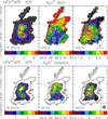 |
Fig. 2. Integrated intensity (moment 0) map of the N2H+ (1–0) main line centered at 93.1737699 GHz (white contours) overlaid on the integrated intensity, line velocity (moment 1), and linewidth (moment 2) maps (colors) for the main line (top panels) and the satellite line centered at 93.1762595 GHz (bottom panels). The line emission has been integrated over the velocity range 93 to 98 km s−1. The white contours range from 0.2 K km s−1 to 6.2 K km s−1 by 1.2 K km s−1. The white cross indicates the position of the dust continuum emission peak of the G31 HMC. The black dashed line in the velocity maps indicates the direction of the NE–SW velocity gradient observed in the G31 HMC in several high-density tracers at high-angular resolution (e.g., Beltrán et al. 2018). The IRAM 30m beam is shown in the lower right-hand corner of the bottom right panel. |
The line velocity maps (Fig. 2) show a clear NNE–SSW velocity gradient across the cloud extending over nearly 5 pc, from the northern to the southern filaments that suggests global motions in the cloud. The value of the velocity gradient is ∼0.4 km s−1 pc−1. The linewidth toward the position of the G31 HMC/protocluster (P1), that is to say in the inner 1 pc of the hub region, is 2.5–3 km s−1 as estimated from the satellite line (F1 = 0–1). We note that the linewidth toward the HMC estimated from the main line (12, 3−01, 2) (right upper panel in Fig. 2) should be taken as an upper limit because this line is optically thick as compared to the satellites. In addition, the main transition is blended with other F1 = 2–1 hyperfine transitions, as shown in Table A.2. The linewidth along the filaments and within the southern emission peak P2 (lacking young stellar objects) is very small, with values of ≲1 km s−1.
4. Discussion
4.1. Kinematics at large scale
The velocity line maps of N2H+ have revealed the existence of a clear NNE–SSW velocity gradient at a large scale in the region (Fig. 2). The direction of this velocity gradient, especially as seen in the optically thinner satellite line, matches that of the well-known gradient (at scales of < 0.1 pc) observed in several high-density tracers, such as CH3CN, at high-angular resolution (better than 1″ or 3750 au) toward the G31 HMC (Beltrán et al. 2004, 2005, 2018; Girart et al. 2009; Cesaroni et al. 2011) and interpreted as rotation of the core. The direction of the small-scale velocity gradient is indicated with a dashed line in Fig. 2. We have identified two possible origins for the gradient: rotation and cloud-cloud collision. A gradient of ∼0.4 km s−1 pc−1 at scales of ∼5 pc, if interpreted as rotation, would correspond to an angular rotation Ω of ∼1.3 × 10⁻¹⁴ s−1. This corresponds to a rotation period of ∼15 × 106 yr and would need a central mass of ∼600 M⊙ for a rotation radius of ∼2.5 pc. Cesaroni et al. (2011) estimated a mass of ∼400 M⊙ for the G31 HMC, which is, however, not concentrated at the center of the cloud. Therefore, although rotation may be supported, it is unlikely that gas on parsec scales has been revolving for about 15 million years around a 600 M⊙ star cluster concentrated at the center of the system.
The most likely explanation for the large-scale velocity gradient is a cloud-cloud collision. In this scenario, the filaments in G31 visible in absorption in the near-IR and in emission in N2H+ and far-IR continuum would have formed by compression resulting from the collision (e.g., Inoue & Fukui 2013), and the rotation of the HMC observed at scales of 1000 au would have been induced by shear caused by the cloud-cloud collision (Balfour et al. 2015, 2017). According to Kumar et al. (2020), cloud-cloud collision could be the most likely mechanism through which hubs with large networks of filaments form in massive clouds (see also, Balfour et al. 2015; Fukui et al. 2021). The material is conveyed from the large-scale cloud to the hubs through these filaments and this leads to cluster formation, as observed in other high-mass star-forming regions, such as SDC13 (Peretto et al. 2014) and G14.2 (Chen et al. 2019). In this scenario, the hub gains a twist as the point where the filaments intersect is different from the center of mass.
The cloud-cloud collision scenario is supported by the fact that the N2H+ spectra show two velocity components toward the HMC (see Fig. 1 and Table A.2), while only one velocity component is visible at all the other positions. The spatial resolution of the observations here is insufficient to trace the longitudinal flows along the filaments as observed in other high-mass star-forming regions, such as SDC13 (Peretto et al. 2014) and G14.2 (Chen et al. 2019). However, one can estimate the mass available in the filaments that could still be incorporated in the central hubs. For this we have used the N2H+ mean column density of 4.1 × 1012 cm−2, estimated in an area of ∼4600 arcsec2 for the most clear filament in the region, the northern filament or region A in Fig. 1 and Table A.2. Assuming an N2H+ abundance of ∼2.5 × 10⁻¹⁰ (Hacar et al. 2017), the mass available in this filament is ∼460 M⊙.
4.2. G31: A benchmark for the F2C paradigm
We would like to note that N2H+ and far-IR observations suggest that G31 could represent a typical example of HFS, where star-formation is explained in terms of the F2C paradigm postulated by Kumar et al. (2020, 2022). In this scenario, the elongated and flattened hub is located at the center of two, nearly equal-sized lobes of the bipolar-shaped radiation bubble visible in the IR (Fig. 1), and it is fed by material conveyed though the filaments (see the sketch in Fig. 3). The HFS shows two N2H+ emission peaks located on either side of the hub center (Fig. 2), one located at the position of the HMC G31, where a massive protocluster has already formed (Beltrán et al. 2021), and the other to the south, which could be the next site of massive star formation. These dense cores have also been observed in dust continuum emission with Herschel from 160 μm to 500 μm, and they are similar to the two centers of activity in a flattened hub described by the F2C paradigm (Kumar et al. 2022), where one center is at an earlier evolutionary stage than the other.
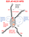 |
Fig. 3. Sketch of the evolutionary stage of G31 within the F2C paradigm (Kumar et al. 2020). A hub is formed by the junction of filaments. The hub gravitational potential triggers and drives longitudinal flows, bringing additional matter and further enhancing the density. Hub fragmentation results in two star formation sites with different ages. Radiation pressure and ionization feedback escapes through the interfilamentary cavities by punching holes in the flattened hub. |
The fact that the HMC with its associated massive protocluster is located close (∼5″) to a more evolved UC HII region, ionized by an O6 star, suggests that G31 could be in transition between Stage III and IV (Fig. 3) of the evolutionary scenario proposed by Kumar et al. (2020). This hypothesis is supported by the fact that IR emission bubbles, which could indicate ultraviolet radiation escaping through the interfilamentary cavities, are already visible (Fig. 1) as in Stage IV. However, the fact there are still no visible pillars suggests that this hub is still in a phase prior to Stage IV. Taking the morphology of the region into account, G31 could represent an edge-on view of the HFSs described by Kumar et al. (2020) in an intermediate phase stage between III and IV. In contrast, Mon R2 (Kumar et al. 2022) represents a face-on view of a system similar to G31.
Dust polarization observations of G31 carried out with the Submillimeter Array (SMA) at 1″ (Girart et al. 2009) and the Atacama Large Millimeter/submillimeter Array (ALMA) at 0.02″ (Beltrán et al. 2019) have revealed an hourglass-shaped magnetic field in a HMC with the symmetry axis roughly coinciding with the plane of the hub. This is consistent with the predictions of Kumar et al. (2020, 2022), who propose that the accretion of material and the density increase in the hub would compress the initial and local magnetic field. This would increase the magnetic field strength, which in the G31 HMC is on the order of ∼10 mG (Beltrán et al. 2019); this would also stabilize the hub against multiple fragmentation into low-mass objects and favor fragmentation into fewer high-mass objects with similar masses, as observed in G31 (Beltrán et al. 2021).
5. Conclusions
G31 represents a typical example of a hub-filament system and a benchmark for the filaments-to-clusters paradigm of star formation. IRAM 30m N2H+ observations suggest that star formation in the G31 cloud has started by a cloud-cloud collision, which has led to the formation of the hub-filament system, and ultimately to cluster formation associated with the hot molecular core. In this massive star formation scenario, the rotation of the G31 HMC observed at scales of a few 1000 au would have been induced by shear caused by the cloud-cloud collision at scales of a few parsecs.
Madrid Data Cube Analysis on ImageJ is a software developed at the Center of Astrobiology (CAB) in Madrid; http://cab.inta-csic.es/madcuba/Portada.html
Acknowledgments
This work is based on observations carried out under project number 049−21 with the IRAM 30m telescope. IRAM is supported by INSU/CNRS (France), MPG (Germany) and IGN (Spain). We are grateful to the IRAM 30m staff for their help during the different observing runs. V.M.R. acknowledges support from the Comunidad de Madrid through the Atracción de Talento Investigador Modalidad 1 (Doctores con experiencia) Grant (COOL: Cosmic Origins Of Life; 2019-T1/TIC-15379).
References
- Balfour, S. K., Whitworth, A. P., Hubber, D. A., & Jaffa, S. E. 2015, MNRAS, 453, 2471 [Google Scholar]
- Balfour, S. K., Whitworth, A. P., & Hubber, D. A. 2017, MNRAS, 465, 3483 [NASA ADS] [CrossRef] [Google Scholar]
- Beltrán, M. T., Cesaroni, R., Neri, R., et al. 2004, ApJ, 601, L190 [Google Scholar]
- Beltrán, M. T., Cesaroni, R., Neri, R., et al. 2005, A&A, 435, 901 [Google Scholar]
- Beltrán, M. T., Codella, C., Viti, S., Neri, R., & Cesaroni, R. 2009, ApJ, 690, L93 [Google Scholar]
- Beltrán, M. T., Cesaroni, R., Rivilla, V. M., Sánchez-Monge, Á., et al. 2018, A&A, 615, A141 [NASA ADS] [CrossRef] [EDP Sciences] [Google Scholar]
- Beltrán, M. T., Padovani, M., Girart, J. M., Galli, D., et al. 2019, A&A, 630, A54 [NASA ADS] [CrossRef] [EDP Sciences] [Google Scholar]
- Beltrán, M. T., Rivilla, V. M., Cesaroni, R., et al. 2021, A&A, 648, A100 [Google Scholar]
- Caselli, P., Myers, P. C., & Thaddeus, P. 1995, AJ, 455, L77 [NASA ADS] [Google Scholar]
- Cazzoli, G., Cludi, L., Buffa, G., & Puzzarini, C. 2012, ApJS, 203, 11 [NASA ADS] [CrossRef] [Google Scholar]
- Cesaroni, R., Beltrán, M. T., Zhang, Q., Beuther, H., & Fallscheer, C. 2011, A&A, 533, A73 [NASA ADS] [CrossRef] [EDP Sciences] [Google Scholar]
- Chen, H.-R. V., Zhang, Q., Wright, M. C. H., et al. 2019, ApJ, 875, 24 [Google Scholar]
- Colzi, L., Rivilla, V. M., Beltrán, M. T., et al. 2021, A&A, 653, A129 [NASA ADS] [CrossRef] [EDP Sciences] [Google Scholar]
- Endres, C. P., Schlemmer, S., Schilke, P., et al. 2016, J. Mol. Spectrosc., 327, 95 [NASA ADS] [CrossRef] [Google Scholar]
- Fukui, Y., Habe, A., Inoue, T., et al. 2021, PASJ, 73, S1 [NASA ADS] [CrossRef] [Google Scholar]
- Girart, J. M., Beltrán, M. T., Zhang, Q., Rao, R., & Estalella, R. 2009, Science, 324, 1408 [NASA ADS] [CrossRef] [Google Scholar]
- Hacar, A., Tafalla, M., & Alves, J. 2017, A&A, 606, A123 [NASA ADS] [CrossRef] [EDP Sciences] [Google Scholar]
- Hacar, A., Tafalla, M., Forbrich, J., et al. 2018, A&A, 610, A77 [NASA ADS] [CrossRef] [EDP Sciences] [Google Scholar]
- Havenith, M., Zwart, E., Meerts, W. L., & ter Meulen, J. J. 1990, J. Chem. Phys., 93, 8446 [NASA ADS] [CrossRef] [Google Scholar]
- Immer, K., Li, J., Quiroga-Nuñez, L. H., et al. 2019, A&A, 632, A123 [NASA ADS] [CrossRef] [EDP Sciences] [Google Scholar]
- Inoue, T., & Fukui, Y. 2013, ApJ, 774, L31 [Google Scholar]
- Jackson, J. M., Rathborne, J. M., Shah, R. Y., et al. 2006, ApJS, 163, 145 [NASA ADS] [CrossRef] [Google Scholar]
- Kumar, M. S. N., Palmeirim, P., Arzoumanian, D., & Inutsuka, S. I. 2020, A&A, 642, A87 [EDP Sciences] [Google Scholar]
- Kumar, M. S. N., Arzoumanian, D., M’enshchikov, A., et al. 2022, A&A, 658, A114 [NASA ADS] [CrossRef] [EDP Sciences] [Google Scholar]
- Martín, S., Martín-Pintado, J., Blanco-Sánchez, C., et al. 2019, A&A, 631, A159 [Google Scholar]
- Mininni, C., Beltrán, M. T., Rivilla, V. M., et al. 2020, A&A, 644, A84 [NASA ADS] [CrossRef] [EDP Sciences] [Google Scholar]
- Molinari, S., Swinyard, B., Bally, J., et al. 2010, A&A, 518, L100 [NASA ADS] [CrossRef] [EDP Sciences] [Google Scholar]
- Müller, H. S. P., Thorwirth, S., Roth, D. A., & Winnewisser, G. 2001, A&A, 370, L49 [Google Scholar]
- Peretto, N., Fuller, G. A., André, Ph., et al. 2014, A&A, 561, A83 [NASA ADS] [CrossRef] [EDP Sciences] [Google Scholar]
- Rivilla, V. M., Beltrán, M. T., Cesaroni, R., et al. 2017, A&A, 598, A59 [NASA ADS] [CrossRef] [EDP Sciences] [Google Scholar]
Appendix A: Physical parameters of the gas derived from N2H+
We used the N2H+ spectroscopy from the Cologne Database for Molecular Spectroscopy (CDMS) catalog4 (Müller et al. 2001; Endres et al. 2016) entry 029506 (version 4, April 2014) based on the works by Caselli et al. (1995) and Cazzoli et al. (2012) and the dipole moment from Havenith et al. (1990). The J=1−0 transition splits into fifteen different hyperfine transitions due to the interactions between the molecular electric field gradient and the electric quadrupole moment of the two nitrogen nuclei. Table A.1 shows information about the hyperfine transitions, obtained from the hyperfine entry from CDMS. The partition function takes the 14N hyperfine splitting into account
N2H+ spectroscopy used in the analysis.
LTE analysis of the molecular emission toward selected regions (see Fig. 1)a.
All Tables
All Figures
|
Fig. 1. Total N2H+ (1–0) emission integrated between 80 and 110 km s−1 overlaid on the wide-field IR Spitzer 8 μm image of the G31 star-forming region (middle panel). The coordinates are J2000 right ascension and declination. The white contours show emission levels from 0.5 to 3 K km s−1 (in steps of 0.5 K km s−1), and from 4 to 24 K km s−1 (in steps of 2 K km s−1). The red dots and the red dashed areas denote selected positions and regions, respectively, whose spectra are shown in the left and right panels. Left and right panels: N2H+ (1–0) spectra (gray histograms) toward selected positions and regions. The red curves show the best LTE fit obtained with MADCUBA. Blue and green curves in P1 show the two velocity components that better fit the data. The vertical dashed line corresponds to v − v0 = 0, where v0 is the systemic velocity of 96.5 km s−1 (Beltrán et al. 2018). The y-axis scale shows the main beam temperature, TB, in K, at the peak positions (P1 and P2) or averaged within the regions (F1, F2, F2, and F4). |
| In the text | |
|
Fig. 2. Integrated intensity (moment 0) map of the N2H+ (1–0) main line centered at 93.1737699 GHz (white contours) overlaid on the integrated intensity, line velocity (moment 1), and linewidth (moment 2) maps (colors) for the main line (top panels) and the satellite line centered at 93.1762595 GHz (bottom panels). The line emission has been integrated over the velocity range 93 to 98 km s−1. The white contours range from 0.2 K km s−1 to 6.2 K km s−1 by 1.2 K km s−1. The white cross indicates the position of the dust continuum emission peak of the G31 HMC. The black dashed line in the velocity maps indicates the direction of the NE–SW velocity gradient observed in the G31 HMC in several high-density tracers at high-angular resolution (e.g., Beltrán et al. 2018). The IRAM 30m beam is shown in the lower right-hand corner of the bottom right panel. |
| In the text | |
|
Fig. 3. Sketch of the evolutionary stage of G31 within the F2C paradigm (Kumar et al. 2020). A hub is formed by the junction of filaments. The hub gravitational potential triggers and drives longitudinal flows, bringing additional matter and further enhancing the density. Hub fragmentation results in two star formation sites with different ages. Radiation pressure and ionization feedback escapes through the interfilamentary cavities by punching holes in the flattened hub. |
| In the text | |
Current usage metrics show cumulative count of Article Views (full-text article views including HTML views, PDF and ePub downloads, according to the available data) and Abstracts Views on Vision4Press platform.
Data correspond to usage on the plateform after 2015. The current usage metrics is available 48-96 hours after online publication and is updated daily on week days.
Initial download of the metrics may take a while.