© ESO 2022

1 Introduction

Our previous work in Sutinjo et al. (2021, hereafter Paper I) discussed a formulation for the sensitivity in terms of system equivalent flux density (SEFD) for a polarimetric interferometer that consists of dual-polarized antennas. In that work we provided an example using a dual-polarized MWA dipole element embedded in an array. In this paper, we extend and generalize the SEFD formulation to polarimetric phased arrays interferometers. This is an important generalization as it is directly applicable to low-frequency interferometric phased array telescopes in operation such as the Murchison Widefield Array (MWA; Tingay et al. 2013) and Low-Frequency Array (LOFAR; van Haarlem et al. 2013), as well as the future Low Frequency Square Kilometre Array (SKA-Low; Labate et al. 2017a,b). In particular regarding the SKA-Low, a clear conceptual understanding of array sensitivity, how it varies over telescope pointing angles, and how to calculate it are crucial for validation against SKA sensitivity requirements (Caiazzo 2017).

The reasons for using SEFD as the valid figure of merit (FoM) for a polarimetric radio interferometer as opposed to antenna effective area on system temperature (A_e/T_sys) was thoroughly reviewed in Paper I. For convenience, we mention the key ideas here. The primary reason is that antenna effective area, A_e, is a number that is defined as matched to the polarization of the incident wave, which is not known in advance for a polarimeter. In contrast, the concept of equivalent flux density is not constrained to the polarization state and it can be readily equated to the system noise. The work in Paper I allowed us to demonstrate that the often-used conversion between A_e/T_sys and SEFD is only an approximation that is valid in certain cases where the Jones matrix is diagonal or anti-diagonal. This is further generalized in the current paper (see Sect. 2.5), where we show that the SEFD approximation is correct only for row vectors in the Jones matrix (see Eq. (1)) that are orthogonal. When the row vectors are not orthogonal, the root-mean-square (rms) SEFD approximation always underestimates the true SEFD.

Furthermore, in our work on this subject we make an explicit connection to observational radio interferometry which is demonstrated by comparison to radio images. We also calculated and conducted a careful review of second-order noise statistics that form the basis for the SEFD formula. These are the main differences between our work and existing work in the radio astronomy phased array sensitivity literature, for example Warnick et al. (2012), Ellingson (2011), Tokarsky et al. (2017), and Sutinjo et al. (2015). However, we acknowledge that there are aspects of our calculations that benefit from the pre-existing collective knowledge in the community, in particular regarding the computation of array response to an incident wave and array noise temperature, as discussed in Sects. 2.1 and 2.3.

The polarimetric phased array under consideration has N dual-polarized elements where each element is connected to a low-noise amplifier (LNA), as is typical in practice. The LNA outputs are connected to the phased array weights and subsequently summed to produce the array output shown in Fig. 1. We consider the array response to an incident electric field from a target direction, e_t. The voltages that represent the response of Array 1 are

$$\begin{array}{l}{\text{v}}_1|{}_t={\text{Je}}_t,\hfill \\ \left[\begin{array}{l}{v}_{X1}|{}_t\hfill \\ v_{Y1}|{}_t\hfill \end{array}\right]=\left[\begin{array}{l}{l}_{X\theta }{l}_{X\varphi }\hfill \\ l_{Y\theta }{l}_{Y\varphi }\hfill \end{array}\right]\left[\begin{array}{l}{E}_{t\theta }\hfill \\ E_{t\varphi }\hfill \end{array}\right],\hfill \end{array}$$(1)

where V_X1 and V_Y1 are the voltages measured by the X and Y arrays, respectively, and J is the Jones matrix of the array; the elements of the Jones matrix are antenna lengths (in meters) that represent the response of the array to each polarization basis of the electric field, E_tθ, E_tϕ (in units of Vm⁻¹). There is a similar equation corresponding to Array 2. For antenna arrays of an identical design, it is reasonable to assume the same Jones matrix as Array 1.

Equation (1) is applicable to an array of antennas. We consider an array of dual-polarized antennas with outputs that are weighted and summed, then connected to a correlator as depicted in Fig. 1, thereby forming an interferometer. The antennas receive noise from the sky which includes a partially polarized target source ${\overline{E}}_{\text{t}}$ and a background with noise temperature distribution given by T_sky. For brevity, only four elements are shown per array. The extension to N elements is immediately evident. The LNAs, represented by the triangle gain blocks, produce their own noise which is scattered by the array and picked up by all elements in the array. Similarly, the incident sky signal arriving at the array undergoes the same scattering and coupling process. Therefore, the combined noise voltages seen at the LNA inputs are mutually correlated. We consider these noise sources and the interactions thereof to extend the SEFD formula to the interferometric and polarimetric phased array telescope.

This paper is organized as follows. The SEFD derivation and calculation are presented in Sect. 2. An example SEFD calculation procedure for the MWA is demonstrated in Sect. 3. The SEFD calculation is validated by MWA observations described in Sect. 4, with comparison and discussion given in Sect. 5. The concluding remarks are summarized in Sect. 6. The appendix presents a detailed review of fundamental assumptions and statistical calculations that justify the SEFD formula presented in Sect. 2.

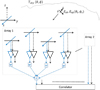Fig. 1 Arrays of dual-polarized low-frequency antennas observing the sky. The antennas are at fixed positions above the ground, and the z-axis is up. The signal from each element is amplified by an LNA, weighted, and summed. The output of each summation is directed into the correlator. The y-directed elements (black) follow the same signal flow, but are not shown. A four-element array is shown as an example.

2 SEFD of a polarimetric phased array interferometer

2.1 Jones matrix of a dual-polarized array

The calculations in Paper I are reusable for an array, but need reinterpretation and adaptation which we now discuss. The first modification is to take the direction-dependent antenna lengths seen in the array environment (i.e., where each antenna element is connected to the input of an LNA). We call this quantity the antenna’s “realized length” (Ung et al. 2020; Ung 2020) which is different from the open circuit antenna effective length in Paper I.

The realized length has the advantage of having a clear and physical interpretation in an array environment depicted in Fig. 2. It is obtained by summing the embedded element realized lengths to form an overall equivalent realized length for the array. For example, for the X array,

$$\begin{array}{l}{l}_{X\theta }=w_x^T{l}_{x\theta },\hfill \\ l_{X\varphi }=w_x^T{l}_{x\varphi },\hfill \end{array}$$(2)

where $w_x^T=[w_{1x},\dots ,w_{4x}]$ is the vector of weights and $l_{x\theta }^T=[l_{1x\theta },\dots ,l_{4x\theta }]$ is a vector containing the embedded element realized lengths, and similarly with l_xϕ. The quantities l_1xθ and l_1xϕ are obtained for a dual-polarized embedded element (number 1) with all other elements in the array terminated with the LNA input impedance, Z_LNA, as shown in Fig. 2. The embedded antenna realized length can be obtained through full-wave electromagnetic simulation (Ung et al. 2020) or measurement. Similarly, for the Y array, $$\begin{array}{l}{l}_{Y\theta }=w_y^T{l}_{y\theta },\hfill \\ l_{Y\varphi }=w_y^T{l}_{y\varphi }\hfill \end{array}$$(3)

where $w_y^T=[w_{1y},\dots ,w_{4y}]$ is the vector of weights for the Y array, which may differ from w_x. We note that Eqs. (2) and (3) apply to the antenna realized length as we noted earlier, as opposed to the open-circuit length. We assume LNAs of an identical design in this paper, and hence the LNA voltage gains are identical and need not be explicitly shown in Eq. (1).

Given the above discussion regarding the realized length, then for a phased array, the voltages on the left-hand side of Eq. (1) represent those at the outputs of the summation shown in Fig. 1. Therefore, the Jones matrix, J, translates the incident field to the voltages at the outputs of the summation. This is similarly the case for Array 2 in Fig. 1. The entries of J represent the realized lengths of the array (for the X or Y component) to an electric field basis ($\widehat{\theta }$ or $\widehat{\varphi }$) such that each entry is a linear combination of the realized lengths of the embedded elements in the array. The Jones matrix then, is $$\text{J}=\left[\begin{array}{l}{l}_{X\theta }{l}_{X\varphi }\hfill \\ l_{Y\theta }{l}_{Y\varphi }\hfill \end{array}\right]=\left[\begin{array}{l}{w}_x^T{l}_{x\theta }{w}_x^T{l}_{x\varphi }\hfill \\ w_y^T{l}_{y\theta }{w}_y^T{l}_{y\varphi }\hfill \end{array}\right].$$(4)

We adopt the uppercase X or Y to denote the overall array response and lower case x or y for the embedded elements in the array.

Fig. 2 Antenna length calculation for an array, where l1xθ is the antenna length associated with $\widehat{\theta }$ polarized incident field for x-directed antenna in the embedded element number 1 in the array shown, similarly to lixθ, liyθ, where i is the embedded element number. For brevity we consider a four-element array i = 1, ⋯, 4; the extension to i = 1, ⋯, N presents no complication.

2.2 SEFD expression

The interferometric polarimeter estimates the outer product of the incident electric field in the target direction, which from Paper I is given by $$\tilde{e}{\tilde{e}}^H={\text{J}}^{-1}{\text{v}}_1{\text{v}}_2^H{\text{J}}^{-H}$$(5)

where J is defined by Eq. (4), which represents the response of the array. The SEFD is proportional to the standard deviation of the flux estimate $${\text{SEFD}}_I=\frac{\text{SDev}(\tilde{I})}{{\eta }_0}=\frac{\text{SDev}\left[{(\tilde{e}{\tilde{e}}^H)}_{1,1}+{(\tilde{e}{\tilde{e}}^H)}_{2,2}\right]}{{\eta }_0}$$(6)

where _1,1,_2,2 indicate the diagonal entries of the matrix in Eq. (5) (hence the subscript I, which refers to Stokes I) and η₀ ≈ 120π Ω is the free space impedance. What is needed is the expression for the standard deviations (SDev) for the phased array interferometer, which we develop next.

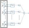Fig. 3 Diagram representing system noise. The array is surrounded by a homogeneous blackbody radiator at temperature Tsys that represents the diffuse sky noise and the LNA noise. The y elements are similarly connected to a separate weight and summing circuit that are not shown for brevity.

2.3 Array system noise

We now compute the standard deviation of the electric field estimates as expressed in Eq. (6) due to the system noise. As shown in Paper I, we expect to express the standard deviation in Eq. (6) in terms of the array realized lengths and the system noise temperatures, T_SyS. Therefore, we need expressions for the mean square voltages for the X and Y arrays due to the system noise.

Figure 3 depicts an array illuminated by an equivalent homogeneous blackbody environment at temperature T_SyS The value of T_SyS is that which equals the noise due to the actual diffuse background sky under observation, T_sky, plus the noise of the LNAs (T_rcv) in the array environment, and the ohmic loss which is a function of the radiation efficiency (η_rad) of the array. The T_SyS value for a phased array can be obtained through computation, measurements, or a combination of the two using well-documented procedures. For example, computation for T_rcv of an array was discussed in the literature (Warnick et al. 2009; Belostotski et al. 2015; Warnick et al. 2018; Ung et al. 2019a, 2020). The computation of T_SyS for the MWA was demonstrated in Ung et al. (2020) and Ung (2020) and was validated by observation. The T_SyS value could also be obtained through measurements by carefully calibrating the array gain via known hot and cold sources (see, e.g., Chippendale et al. 2014).

The T_sys for the X and Y arrays are generally different; this is similarly noted in Paper I for a dual-polarized antenna element. This is expected because for the same sky under observation, the X and Y arrays produce different responses on the sky. Moreover, the x elements and the y elements interact differently depending on the array configuration and weights. Therefore, we anticipate assigning different T_sysX and T_sysY to the respective arrays, which we discuss next.

An equivalent homogeneous sky at T_sys gives rise to partially correlated noise voltages at the antenna ports in the array. A convenient way to quantify this is to start with the case where each antenna port is terminated with an open circuit: Z_LNA → ∞. In this case, the mutual coherence is known from the generalized Nyquist theorem (Twiss 1955; Hillbrand & Russer 1976) $${\text{C}}_o{|}_{T_{\text{sys}}}=\langle {\text{v}}_o{\text{v}}_o^H\rangle {|}_{T_{\text{sys}}}=4k{T}_{\text{sys}}\Delta f\Re [\text{Z}]$$(7)

where Δf is the noise bandwidth and ℜ[Z] is the real part of the antenna impedance matrix, which is a real and symmetric matrix. We chose the port numbering convention such that $$\Re [\text{Z}]=\Re \left[\begin{array}{l}{\text{Z}}_{xx}{\text{Z}}_{xy}\hfill \\ {\text{Z}}_{yx}{\text{Z}}_{yy}\hfill \end{array}\right],$$(8)

that is the x_ı, ⋯, x₄ embedded elements ports are numbered 1 to 4 and the y₁, ⋯, y₄ embedded elements ports are numbered 5 to 8, such that the open circuit voltage vector is $v_o^T=[V_{ox1},\cdots ,V_{ox4},V_{oy1},\cdots ,V_{oy4}]$. The open circuit voltage vector is related to the voltage seen at the LNA inputs through a transformation matrix (Warnick et al. 2009), which we call T, such that $$\text{v}=Z_{\text{LNA}}{[Z_{\text{LNA}}I+Z]}^{-1}{\text{v}}_O=T{v}_O$$(9)

Therefore, the coherence matrix of the voltages seen at the inputs of the LNAs loaded with Z_LNA is $$\begin{array}{l}T{\text{C}}_o{|}_{T_{\text{sys}}}{T}^H=T\langle {\text{v}}_o{\text{v}}_o^H\rangle {|}_{T_{\text{sys}}}{T}^H\hfill \\ =4k{T}_{\text{sys}}\Delta fT\Re [\text{Z}]{\text{T}}^H,\hfill \end{array}$$(10)

which is a Hermitian matrix, since (Tℜ[Z]T^H)^H = Tℜ[Z]T^H.

The sought-after quantities are the mean square voltages after weighting and summing $$\begin{array}{c}\langle |V_X{|}^2\rangle =[w_x^T,0_4^T]{\text{TC}}_o{|}_{T_{\text{sys}}{}_{\text{X}}}{\text{T}}^H\left[\begin{array}{l}{w}_x^{*}\hfill \\ 0_4\hfill \end{array}\right]\\ =4k{T}_{\text{sysX}}\Delta f{w}_{x0}^{T}T\Re [\text{Z}]T^H{w}_{x0}^{*}\\ \langle |V_Y{|}^2\rangle =[0_4^T,w_y^T]T{\text{C}}_o{|}_{T_{\text{sysY}}}{T}^H\left[\begin{array}{l}{0}_4\hfill \\ {\text{w}}_y^{*}\hfill \end{array}\right]\\ =4k{T}_{\text{sysY}}\Delta f{\text{w}}_{y0}^T\text{T}\Re [\text{Z}]{\text{T}}^H{w}_{y0}^{*}\end{array}$$(11)

where 0₄ is a column vector of four zeros; w_x0, w_y0 reflect the fact that the x and y antennas are summed separately; T_sysX and T_sysY are distinguished as discussed previously; k is the Boltzmann constant; and Δf is the noise bandwidth. We know that Eq. (11) is real because the eigenvalues of a Hermitian matrix are real. For brevity in the SEFD formula, we adopt the following shorthand notations: $$\begin{array}{c}{R}_X=w_{x0}^{T}T\Re [\text{Z}]T^H{w}_{x0}^{*},\\ R_Y=w_{y0}^T\text{T}\Re [\text{Z}]T^H{w}_{y0}^{*}.\end{array}$$(12)

We can think of them as the realized array noise resistances, in units of Ω, representing the noise voltages at the outputs of the summations. A detailed explanation of this quantity and comparison to current literature can be found in Appendix B. We note that Eq. (11) transforms T_sysX, T_sysY from a quantity external to the array to the mean square voltages after weighting and summing by the array. Therefore, the output of the summation is the reference plane at which the SEFD is to be calculated, as we show next.

2.4 SEFD_I formulation

We assume all the antenna arrays in question are of identical design and the coupling between arrays is negligible due to the inter-array distance of tens of wavelengths or larger. The intra-array coupling within each array is accounted for through the process described in Sects. 2.1 and 2.3. This is the same level of assumptions as in Paper I. The main difference between Paper I and this work is that the sensitivity formula is now extended and generalized to the phased array. Following from Paper I, the Stokes I estimate is $\tilde{I}={(\tilde{e}{\tilde{e}}^H)}_{1,1}+{(\tilde{e}{\tilde{e}}^H)}_{2,2}$ from Eqs. (5) and (6). Expanding the matrix equation, we can write $$\begin{array}{c}|D{|}^2\tilde{I}=X_1{X}_2^{*}(|l_{Y\varphi }{|}^2+|l_{Y\theta }{|}^2)\\ +Y_1{Y}_2^{*}(|l_{X\varphi }{|}^2+|l_{X\theta }{|}^2)\\ -X_1{Y}_2^{*}(l_{X\varphi }^{*}{l}_{Y\varphi }+l_{X\theta }^{*}{l}_{Y\theta })\\ -Y_1{X}_2^{*}(l_{X\varphi }{l}_{Y\varphi }^{*}+l_{X\theta }{l}_{Y\theta }^{*})\end{array}$$(13)

where D = l_Xθl_Yϕ − I_Xϕl_Yθ is the determinant of the array Jones matrix; the leading Vs have been suppressed for brevity; for example, X₁ is a complex random variable that refers to V_Xı. The components of the realized lengths (which are direction-dependent complex scalars) now refer to the array, as discussed in Sect. 2.1. Following the statistical calculation described in Appendix A, $$\frac{|D{|}^4\text{Var}(\tilde{I})}{{(4k\Delta f)}^2}={\text{t}}_R^T\mathbb{L}{\text{t}}_R$$(14)

where $$t_R=\left[\begin{array}{l}{T}_{\text{sysX}}{R}_X\hfill \\ T_{\text{sysY}}{R}_Y\hfill \end{array}\right]$$(15)

is a column vector, and the matrix $$L=\left[\begin{array}{cc}{\Vert l_Y\Vert }^4& {\left|l_{X\varphi }^{*}{l}_{Y\varphi }+l_{X\theta }^{*}{l}_{Y\theta }\right|}^2\\ {\left|l_{X\varphi }^{*}{l}_{Y\varphi }+l_{X\theta }^{*}{l}_{Y\theta }\right|}^2& {\Vert l_X\Vert }^4\end{array}\right],$$(16)

where the vector norms are ${\Vert l_X\Vert }^2={\left|l_{X\theta }\right|}^2+{\left|l_{X\varphi }\right|}^2$ and similarly with ‖l_Y‖². We note in Eq. (14) that R_X and R_Y differ and generally cannot be factored out. Again, taking $\sqrt{\text{Var(}\tilde{I}\text{)}}$ from Eq. (14) and dividing by the free space impedance, η₀, produces the desired formula $${\text{SEFD}}_I=\frac{\text{SDev}(\tilde{I})}{{\eta }_0}=\frac{4k\Delta f}{{\eta }_0}\frac{\sqrt{{\text{t}}_R^T\text{L}{t}_R}}{|D{|}^2}$$(17)

with units Wm⁻². If SEFD_I is stated in Wm⁻² Hz⁻¹, which is often preferred in radio astronomy, then we remove Δf from the right-hand side.

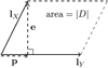Fig. 4 Depiction of the vectors, their projections, and the area of the parallelogram.

2.5 rms approximation always underestimates SEFD

As mentioned in Sect. 1, we now demonstrate the claim that the very commonly used rms approximation in radio astronomy (see, e.g., Wrobel & Walker 1999) always underestimates the true SEFD. The rms approximation is given by $${\text{SEFD}}_I^{\text{rms}}=\frac{1}{2}\sqrt{{\text{SEFD}}_{XX}^2+{\text{SEFD}}_{YY}^2,}$$(18)

where SEFD_XX, SEFD_YY assume an unpolarized source, as discussed in Paper I. For the notations and approach discussed in the current paper, this approximation can be written as $$\begin{array}{c}{\text{SEFD}}_I^{\text{rms}}=\frac{4k}{{\eta }_0}\sqrt{\frac{T_{\text{sysX}}^2{R}_X^2}{\left|\right|l_X|{|}^4}+\frac{T_{\text{sysY}}^2{R}_Y^2}{\left|\right|l_Y|{|}^4}}\\ =\frac{4k}{{\eta }_0}\sqrt{t_R^T{D}_{\text{rms}}{t}_R}\end{array}$$(19)

as pointed out in Paper I. In addition, Appendix C shows that Eq. (19) is derivable using A/T. The diagonal matrix D_rms = diag $\left[{\Vert l_X\Vert }^{-4},{\Vert l_Y\Vert }^{-4}\right]$ is different from $\mathbb{L}/{\left|D\right|}^4$ in Eq. (17). It can be shown that $$t_R^T\frac{\mathbb{L}}{|D{|}^4}{t}_R\ge t_R^T{D}_{\text{rms}}{t}_R$$(20)

The reason for this is explained as follows. It can be shown through the Gram-Schmidt orthogonalization steps or the related QR factorization (Strang 2016, see Chap. 4) of the Jones matrix, that the absolute value of the determinant can be written as $$\left|D\right|=\Vert l_Y\Vert \Vert \text{e}\Vert$$(21)

where e is the projection vector of l_X onto a line which is perpendicular to l_Y (see Fig. 4),

$$\text{e}=l_X-\text{p}$$(22)

where $p=(l_Y^H{l}_X)l_Y/{\Vert l_Y\Vert }^2$ is the orthogonal projection vector of l_X onto l_Y (Strang 2016, see Chap. 4), such that e and p are orthogonal, e ⊥ p. Equation (21) is easily verified by substitution of l_X = [l_Xθ, l_Xϕ]^T and l_Y = [l_Yθ, l_Yϕ]^T into Eq. (22) and simplifying the vector algebra. There is also an insightful geometric interpretation of Eq. (21): |D| is the area formed by the parallelogram whose parallel sides are represented by vectors l_X and l_Y, as shown in Fig. 4; this is known from the volume property of determinants (Strang 2016, see Chap. 5) and is useful for understanding Eq. (23).

Since ‖e‖ ≤‖l_X‖, then $$\begin{array}{l}\text{Since}\Vert \text{e}\Vert \le \Vert l_X\Vert ,\text{then}\hfill \\ |D{|}^2\le {\Vert l_X\Vert }^2{\Vert l_Y\Vert }^2\hfill \end{array}$$(23)

The equality is fulfilled when the vectors are orthogonal, l_Y ⊥ l_X, which also implies p = 0, e = l_X, and $l_X^H{l}_Y$. This is fully

expected given the above-mentioned geometric interpretation and proves Eq. (20). To see this more clearly, we write $$\frac{\mathbb{L}}{|D{|}^4}=\frac{1}{{\Vert l_X-\text{p}\Vert }^4{\Vert l_Y\Vert }^4}\left[\begin{array}{ll}{\Vert l_Y\Vert }^4\hfill & {\Vert l_{{}_X}^H{l}_Y\Vert }^2\hfill \\ {\Vert l_{{}_X}^H{l}_Y\Vert }^2\hfill & {\Vert l_X\Vert }^4\hfill \end{array}\right]$$(24)

and $${\text{D}}_{\text{rms}}=\frac{1}{{\Vert l_X\Vert }^4{\Vert l_Y\Vert }^4}\left[\begin{array}{ll}{\Vert l_Y\Vert }^4\hfill & 0\hfill \\ 0\hfill & {\Vert l_X\Vert }^4\hfill \end{array}\right]$$(25)

We note that the denominator on the right-hand side of Eq. (24), ${\Vert l_X-p\Vert }^4{\Vert l_Y\Vert }^4\le {\Vert l_X\Vert }^4{\Vert l_Y\Vert }^4$, which indeed proves Eq. (20). Furthermore, it is evident that the matrix in Eq. (24) converges to D_rms in Eq. (25) when the orthogonality, l_Y ⊥ l_X, is fulfilled. Since in practice orthogonality is approached, but never fulfilled exactly, the statement that the rms approximation always underestimates SEFD is demonstrably correct.

It is important to note that antenna length is a direction-dependent quantity. Therefore orthogonality, l_Y ⊥ l_X, as discussed in this section must be evaluated by taking the inner product, ${\left|{}_X^H\right|}_Y$, in every direction of arrival of interest. This is particularly applicable to a wide field-of-view antenna system. For example, mechanically orthogonal cross dipoles only possess antenna length orthogonality in the directions of arrival on the cardinal planes (as discussed in Paper I). The rms approximation is only exact in the directions of arrivals for which antenna length orthogonality, ${\left|{}_X^H\right|}_Y=0$, is fulfilled.

Following the proof, we can then quantify this difference by defining a relative percentage difference of the two results as $$\Delta {\text{SEFD}}_I=\frac{{\text{SEFD}}_I-{\text{SEFD}}_I^{\text{rms}}}{{\text{SEFD}}_I}\times 100\%\ge 0$$(26)

We will use Eq. (26) in Sect. 5 to measure the difference between rms approximation and true SEFD based on simulation and observation, the expected value of which are always positive (for observation data, the “expected value” refers to the ensemble mean).

3 SEFD simulation procedure

Following the previous section, the steps to computing the SEFD of a polarimetric phased array interferometer are as follows. The first step involves the computation of the array Jones matrix as shown in Eq. (4). The components of the matrix were constructed from embedded antenna realized lengths as shown in Eqs. (2) and (3), which in our case were obtained from electromagnetic simulation using Altair FEKO¹. Additional information regarding the simulation setup and results used in this paper are discussed in Sokolowski et al. (2017). The embedded antenna realized lengths were found by converting (E_θ, E_ϕ) using (Ung et al. 2020) $$\begin{array}{l}{l}_{n\theta }(\theta ,\varphi )=-j\frac{2\lambda }{{\eta }_0{V}_{\text{t}}}{Z}_{\text{LNA}}{E}_{\theta ,n}(\theta ,\varphi ),\hfill \\ l_{n\varphi }(\theta ,\varphi )=-j\frac{2\lambda }{{\eta }_0{V}_{\text{t}}}{Z}_{\text{LNA}}{E}_{\varphi ,n}(\theta ,\varphi ),\hfill \end{array}$$(27)

where λ is the wavelength, Z_LNA is the input impedance of the low-noise amplifier (LNA), and V_t is the port excitation voltage used during the simulation which generates the corresponding electric far-field components E_θ,n and E_ϕ,n of the n-th embedded element as a function of direction in the sky.

In the second step we determine the system temperatures of the array, T_SySX and T_SySY, using $$T_{\text{sys},\text{p}}=T_{\text{ant},\text{p}}+T_{\text{rcv},\text{p}}+T_0(1-{\eta }_{\text{rad},\text{p}})$$(28)

where T_ant,p is the antenna temperature due to the sky for each polarization p (p = X or Y); T_rcv,p is the receiver noise temperature due to the LNA calculated using the methodology discussed in Ung et al. (2020) based on measured LNA noise parameters (Sutinjo et al. 2018); η_rad,p is the radiation efficiency of the array; and T₀ = 290 K is the reference temperature (which can be substituted by ambient temperature if known). Radiation efficiency, η_rad, is the ratio of the total radiated power to the total injected power into the array calculated using methodologies presented in Warnick et al. (2010) and Ung et al. (2019b).

In the third step we compute the realized array noise resistances, R_X and R_Y, using Eq. (12). Fourth, we calculate ${\text{t}}_R^{T}L{t}_R$ in Eq. (14). Finally, we calculate the polarimetric and interferomet-ric array SEFD using Eq. (17). As an example, we provide several key parameters required to evaluate Eq. (17) at three selected frequency points for an MWA tile pointed at azimuth and zenith angles, Az = 80.54° and ZA = 46.15°, in Table 1. A full list of these values (excluding the realized length) can be found at the CDS. In the next section, we describe the procedure used to obtain SEFD_I from observational data.

4 SEFD measurement procedure

The data analysis procedure is based on a very similar analysis performed earlier (see Paper I). The relative difference $\Delta {\text{SEFD}}_I^{\text{obs}}$ defined by Eq. (26) was measured using MWA observations tracking Hydra-A radio galaxy recorded in a standard observing mode at the central frequency 154.88 MHz. On 2014 December 26 between 16:05:42 and 05:13:42 UTC, the MWA recorded 23 112 s observations centered on the Hydra-A radio galaxy at a position (Az, ZA) = (80.7°, 45.8°) and (Az,ZA) = (290.7°, 32.4°) at the start and end of the observations, respectively. For the purpose of a comparison of ΔSEFD_I between the data and simulations, 52 s of the first 112 s observation (obsID 1103645160 referred to later as ObsA), which started at 201412-26 16:05:42 UTC with Hydra-A at (Az,ZA) = (80.7°, 45.8°), were analyzed. This observation was selected at a pointing direction where the simulation predicted that ΔSEFD_I would be the most prominent due to the lowest elevation of the pointing direction at gridpoint 114 at the elevation of ≈43.85° (zA = 46.15°). We note that MWA observations significantly lower than 45° are generally not routinely performed and were not considered for the presented analysis due to systematic effects which could affect the data quality.

4.1 Calibration and imaging

The MWA data were converted into CASA measurement sets (McMullin et al. 2007) in 40 kHz frequency (total of 768 channels) and 1 s time resolution, and downloaded using the MWA All-Sky Virtual Observatory interface (Sokolowski et al. 2020). In order to avoid aliasing effects at the edges of 1.28 MHz coarse channels (24 in total), 160 kHz (4 fine channels) on each end of the coarse channels were excluded, which reduced the observing bandwidth to R_bw =0.75 fraction of the full recorded band (30.72 MHz).

The same observation ObsA was used for calibration. It was sufficient to use a single-source sky model composed of Hydra-A alone, which was the dominant source in the observed field. However, due to the extended structure of Hydra-A, which is resolved by the longest baselines of the MWA Phase 1, it was necessary to use its model by Lane et al. (2014) converted to the required multi-component format by Hurley-Walker (in prep.)². The total flux density of Hydra-A in this model is within 7% of the most recent and accurate flux measurements of Hydra-A by Perley & Butler (2017) over the entire observing band (139.5 –169.0 MHz). Selecting an appropriate model of Hydra-A was important to ensure the correct flux scale of the calibrated visibilities and images, and ultimately of the SEFD values. The calibration was performed and applied using the CALI-BRATE and APPLYSOLUTIONS software, which are part of the MWA-reduce software package (Offringa et al. 2016) routinely used for MWA data reduction. The CALIBRATE program uses the 2016 MWA beam model (Sokolowski et al. 2017) to calculate the Jones matrices and apparent fluxes of the sources (just one in this particular case) included in the sky model. Baselines shorter than 58 wavelengths were excluded from the calibration. The phases of the resulting calibration solutions were fitted with a linear function, while the amplitudes were fitted with a fifth-order polynomial; the resulting fitted calibration solutions were then applied to the un-calibrated visibilities using the APPLYSOLUTIONS program.

Sky images with 4096 × 4096 pixels of angular size ≈0.6arcmin (image size ≈ 42.2° × 42.2°), in 1 s time resolution, were formed from all correlations products (XX, YY, XY, and YX)³ using the WSCLEAN⁴ program (Offringa et al. 2014). Natural weighting (robust weighting parameter defined by Briggs 1995 set to +2) was used in order to preserve full sensitivity of the array. We note that natural weighting increases the confusion noise, but it was eliminated by measuring the noise from difference images (see Sect. 4.2). The dirty maps were CLEANed with 100 000 iterations and a threshold of 1.2 standard deviations of the local noise. In order to reduce the contribution from extended emission, baselines shorter than 30 wavelengths were excluded, which led to a small reduction in the of number of baselines used in the imaging to 7466, which is R_bs ≈ 0.92 fraction of all the baselines (8128). Corrections for a reduced number of baselines and observing bandwidth were taken into account in the later analysis by applying correction factors (R_bw and R_bs) during the conversion from standard deviation of the noise to SEFD.

The resulting XX and YY images (see left image in Fig. 5) were divided by corresponding images of the beam in X and Y polarizations generated with the 2016 beam model (Sokolowski et al. 2017) at the same pointing direction ((Az, ZA) = (80.5°, 46.2°) at the MWA gridpoint 114⁵). All the resulting images (XX, YY, XY, and YX) were converted to Stokes images (I, Q, U, and V) also using the 2016 beam model. The final products resulting from the above procedure were three sets (XX, YY, and Stokes I) of n_t = 53 primary beam corrected images corresponding to 53 s of the analyzed MWA data.

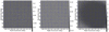Fig. 5 Example 0.5 s sky and difference images in X polarization (scale of the color bar is in Jy) used to calculate SEFD. Left: 0.5 s sky image. Center: difference between two consecutive 0.5 s images. Right: difference between two consecutive 0.5 s images corrected for the primary beam (divided by the primary beam in the X polarization). In order to calculate noise in every direction in the sky within the field of view (noise map), the standard deviation of the noise was calculated in small regions around each pixel in the difference image and divided by $\sqrt{2}$. These noise maps were later converted into SEFD using Eq. (29). The same procedure was applied to Y and is very similar to Stokes I polarizations (in this case the correction for the primary beam was more complex than the simple division by the corresponding primary beam).

4.2 Measuring the SEFD from the noise in the sky images

Using the three series (corresponding to XX, YY, and Stokes I) of n_t = 53 images, difference images (between the subsequent i-th and i - 1 image) were calculated, resulting in n_d = 52 difference images in each of the XX, YY, and Stokes I polarizations. Difference imaging effectively removes confusion noise resulting in uniform images of thermal noise (entirely due to the system temperature T_sys). The difference images were visually inspected and verified to have a uniform noise-like structure (see examples in the middle and right panels of Fig. 5). Therefore, the resulting standard deviation is purely due to the instrumental and sky noise (T_sys).

The standard deviation of the noise calculated in a small region (here a circular region of radius R_n = 10 pixels corresponding to ≈5 synthesized beams) around pixels in the resulting difference images is distributed around a mean of zero and is not contaminated by the variations in the flux density within the circular regions due to astronomical sources contained inside these regions. The interquartile range divided by 1.35 was used as a robust estimator of standard deviation, which is more robust against outlier data points due to radio-frequency interference (RFI) or residuals of astronomical sources in the difference images. Once this calculation was performed around all the pixels in a difference image, an image of the noise over the field of view (FoV) was created. These images of the noise are later referred to as noise maps or just N (which stands for a 2D image and not a number). This procedure was applied to n_d all-sky difference images resulting in n_d noise maps (N_I, N_XX, and N_YY) for each of the polarizations (Stokes I, XX, and YY, respectively). The corresponding SEFD images (2D maps of SEFD) of the entire FoV were calculated from these noise maps (referred to in general as N) according to the equation $$\text{SEFD}=N\sqrt{\Delta v\Delta t{N}_{\text{b}}}$$(29)

where Δt = 1 s is the integration time, Δv = 30.72 × R_bw MHz is the observing bandwidth corrected for reduced number of channels (R_bw) used in the analysis, and N_b = 7466 is the number of baselines used in the imaging.

Noise maps in the three polarizations, N_I, N_XX, and N_YY, were converted into corresponding SEFD_I, SEFD_XX, and SEFD_YY images using Eq. (29), resulting in n_d SEFD images in each polarization (I, XX, and YY). Then, median SEFD images $\overline{{\text{SEFD}}_I,}\overline{SEF{D}_{XX}}$, and $\overline{SEF{D}_{YY}}$ were calculated out of individual n_d SEFD images (a median image of SEFD_I will be shown in Sect. 5.1). These median images were used to calculate $\Delta {\text{SEFD}}_I^{\text{obs}}$ $$\Delta {\text{SEFD}}_I^{\text{obs}}=\frac{\left(\overline{{\text{SEFD}}_I}-\frac{1}{2}\sqrt{{\overline{{\text{SEFD}}_{XX}}}^2+{\overline{{\text{SEFD}}_{YY}}}^2}\right)}{\overline{{\text{SEFD}}_I}}$$(30)

In the next section we provide the results derived from simulated and observed data, and discuss their implications.

4.3 SEFD as a function of frequency

The method described in Sect. 4.1 allows us to determine spatial structure of SEFD by calculating SEFD values in each pixel of 4096 × 4096 sky images. This method was successfully used in Paper I, where a single dipole in each MWA tile was enabled and the remaining 15 dipoles were terminated. However, it has never been applied to measure the SEFD from MWA images resulting from observations in a standard mode with all dipoles in MWA tiles enabled. Therefore, before comparison with the simulations, an initial verification was performed by deriving SEFD values using the well-tested method described in Appendix C (Sutinjo et al. 2015). This method uses the standard deviation of calibrated visibilities to measure SEFD_XX and SEFD_YY as a function of frequency in the direction of Hydra-A source (no spatial information); we note that only the SEFD of instrumental polarizations can be measured using this method, but not SEFD_I. These measurements were used as a reference to confirm that the image-based SEFD values were correct. Furthermore, this method allowed us to compare the frequency dependence of SEFD_XX and SEFD_YY against the simulations. Figure 6 shows the comparison between the observed and simulated results. At the location in the sky corresponding to (Az, ZA) = (80°, 46°), the realized area of the X-polarized dipole is significantly smaller than the Y-polarized dipole, and therefore SEFD_XX is higher than SEFD_YY.

At 154.88 MHz, observed SEFD_XX = 78 ± 7.8 kJy and SEFD_YY = 57.6 ± 3.6 kJy, which is in very good agreement with the values obtained from the imaging method. Overall, there is excellent agreement between simulated and observed SEFD_XX/YY over a wide range of frequencies.

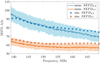Fig. 6 SEFD in the pointing direction of gridpoint 114 with realized area calculated at (Az, ZA) = (80°, 46°) as a function of frequency. The observed SEFD calculated from calibrated visibilities is compared with simulated SEFD.

5 Results and discussion

5.1 Comparison between the data and simulation

In order to ensure that we are able to draw accurate conclusions regarding the difference in SEFD values calculated using the rms approximation in Eq. (18) and the true SEFD using Eq. (17), we compared the simulated SEFD with the measurements. The SEFD of the X, Y, and I using the difference imaging method probes the SEFD over multiple locations in the sky for a given frequency (154.88 MHz). Similarly, the simulated SEFD_XX/YY images were generated using A/T formulation while the simulated SEFD_I image was generated using Eq. (17). Figure 7 shows the SEFD obtained from simulation (Fig. 7a), the Stokes I image (Fig. 7b), and the difference in percentage between the two (Fig. 7c). For reference, contours of the normalized beam pattern for each polarization are displayed in 3 dB increments down to the –12 dB level. The contours of the beam pattern shown in the SEFD_I are obtained by normalizing the reciprocal of Eq. (17). A similar comparison was done for the X and Y polarization, but for brevity the results are included in Appendix D.

The relative difference in percentage, denoted M_SEFD, between the simulated and observed SEFD in all images (XX, YY, and I) was computed as $$M_{\text{SEFD}}=\frac{{\text{SEFD}}^{\text{obs}}-{\text{SEFD}}^{\text{sim}}}{{\text{SEFD}}^{\text{sim}}}\times 100\%$$(31)

We analyzed the errors using histograms, and the observed SEFD_XX and SEFD_I are on average higher by 9 and 4%, respectively, while the observed SEFD_YY is lower by 4% compared to simulated values for all pixels within the −12 dB beam width. Overall, the agreement between the simulated and observed values is within the ±10% range which indicates excellent correspondence between simulated and observed SEFD data.

Following the verification of simulated SEFD with observed data, we were able to calculate the error between the rms and proposed method using Eq. (26). Figures 8a,b show this error for an MWA tile for simulated and observed data, respectively. We can see that the difference between ${\text{SEFD}}_I^{\text{rms}}$ and SEFD_I is not a uniform offset in the image, but has a noticeable structure. For the observation within the −3 dB beam width, the error of SEFD prediction using the rms approximation is only 7%. However, it increases as we move farther away from the beam center and reaches 23% in the −12 dB beam width. We note that for errors in the simulated values, $\Delta {\text{SEFD}}_I^{\text{sim}}$ is always positive, meaning the rms method underestimates the SEFD, which is consistent with the discussion in Sect. 2.5.

Figure 8c shows the subtraction of $\Delta {\text{SEFD}}_I^{\text{obs}}$ and $\Delta {\text{SEFD}}_I^{\text{sim}}$ calculated as $${\Delta }_{\text{sim}/\text{obs}}=\Delta {\text{SEFD}}_I^{\text{obs}}-\Delta {\text{SEFD}}_I^{\text{sim}}$$(32)

The resulting mean difference for all pixels within the −12 dB beam width is zero, which allows us to draw the following conclusions: (i) the negative values seen in $\Delta {\text{SEFD}}_I^{\text{obs}}$ are due to noise and (ii) we can fully predict the amount of underestimation (% errors) in SEFD_I produced by the rms method. This indicates that Eq. (17) more accurately predicts the array’s SEFD_I.

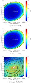Fig. 7 (a) Simulated SEFDI, (b) observed SEFDI, and (c) percentage difference between the simulated and observed SEFDI at 154.88 MHz calculated by Eq. (31).

5.2 Computation of SEFD_I for diagonal plane and low elevation pointing angle

There was a noticeable structure in the result shown in Fig. 8; however, we note that for that observation time, frequency, and pointing angle the difference in SEFD formulation would probably be hard to notice within the 3 dB beam width, and indeed in some cases only images in the target field down to −3 dB are created. Nevertheless, these results show that the improved expression of SEFD_I provides highly accurate SEFD values, and thus can be used to precisely calculate the sensitivity of a radio telescope for any pointing angle within the operating frequency range using simulations.

To this end, it is reasonable to continue our analysis based only on simulated results. We completed an iterative search aimed to find a case where ΔSEFD_I affects the data within −3 dB beam width. Figure 9 shows one outcome of this iterative search. It was found for Az = 45°, ZA = 56.96° (33.04° elevation angle) at 199.68 MHz that the rms SEFD approximation results in a 29% error within the −3 dB beam width and increases up to 36% within the −12 dB beam width. This example further demonstrates the inaccuracies of the rms approximation, which always predicts lower SEFD than the actual value.

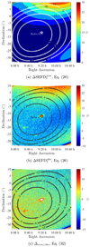Fig. 8 Relative difference between the (a) simulated and (b) observed SEFDI and (c) the difference of $\Delta {\text{SEFD}}_I^{\text{obs}}$ and $\Delta {\text{SEFD}}_I^{\text{sim}}$

6 Conclusion

This work, which is an extension of Paper I, provides a generalized expression of SEFD_I for interferometric phased array polarimeters. As in Paper I, this expression was derived by performing statistical analysis on the standard deviation of the flux density estimate. Our current work further clarifies that the SEFD_I expression does not depend on assumptions made regarding the background polarization or orthogonality in the antenna elements. The key array parameters were obtained from the full-wave electromagnetic simulation of the phased array of interest, which is a MWA tile in this example, and was used to compute SEFD_I given by Eq. (17). The mean percentage difference $\left(M{\text{SEFD}}_I\right)$ between simulated and observed SEFD_I is 4%, which indicates excellent agreement. Furthermore, we provided proof that the rms approximation always underestimates the SEFD_I. This proof also demonstrates that the equality between the rms approximation and SEFD_I is reached when the row vectors in the Jones matrix are orthogonal, which is a condition that can be approached but never fulfilled in practice.

After verifying the accuracy of our simulation with the observed data, we proceeded to compare the relative percentage difference in SEFD_I, as defined in Eq. (26), calculated by the often-used rms approximation and Eq. (17). A large percentage difference here would indicate that the rms approximation underestimates the SEFD_I. We saw that for our chosen observation, the maximum simulated error $\Delta {\text{SEFD}}_I^{\text{sim}}=7\%$ within the –3 dB beam width and increases to 23% within the –12 dB beam width. This result was also verified against the observed data $\left(\Delta {\text{SEFD}}_I^{\text{obs}}\right)$ by taking the absolute difference between the two images (Figs. 8a,b) defined in Eq. (32). The resulting difference between simulated and observed ΔSEFD_I has a zero mean value, which indicates a remarkable agreement between the results.

As we had thoroughly validated our simulation against observed data, we then performed an iterative search for pointing angles and frequencies that would yield a higher difference between the rms approximation and Eq. (17). We found that for beam pointing (Az, ZA) = (45°, 56.96°) at 199.68 MHz the rms approximation produces an error of 29% in $\Delta {\text{SEFD}}_I^{sim}$ within the –3 dB beam width, which increases to 36% within the –12 dB beam width. This outcome is in agreement with the prediction made in Paper I whereby the difference increases at Az = 45^° at low elevation angles.

We conclude that the derived SEFD_I expression improves the fundamental understanding of instrument performance and can be used to accurately calculate sensitivity not only at the principal planes, but also at the diagonal planes (Az = 45^°) and low elevation angles. This enables us to more confidently predict sensitivity for detection of pulsars, fast radio bursts (FRBs), or epoch of reionization (EoR) signal. This is particularly important for the cases where the target sources can only be observed at very low elevations (e.g., in response to alerts about FRBs or any other transient sources).

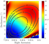Fig. 9 $\Delta {\text{SEFD}}_I^{\text{sim}}$ computed for 199.68 MHz at (Az, ZA) = (45°, 56.96°) showing the impact of the error resulting from the rms expression of SEFDI.

Acknowledgements

This scientific work makes use of the Murchison Radio-astronomy Observatory (MRO), operated by CSIRO. We acknowledge the Wajarri Yamatji people as the traditional owners of the Observatory site. Support for the operation of the MWA is provided by the Australian Government (NCRIS), under a contract to Curtin University administered by Astronomy Australia Limited. This work was further supported by resources provided by the Pawsey Supercomputing Centre with funding from the Australian Government and the Government of Western Australia. The authors thank A/Prof. R. B. Wayth and Prof. D. Davidson for discussions on this topic and for reviewing the draft manuscript. The authors thank Dr. Natasha Hurley-Walker for providing the model of the Hydra-A calibrator source.

Appendix A Statistical Analysis of Var$\left(\tilde{I}\right)$

The statistical reasoning and the vanishing covariance are similar those presented in the Appendix in Paper I. In the current paper, we were able to reduce the assumptions only to the most fundamental ones, namely zero mean Gaussian noise with independent and identically distributed real and imaginary parts (in phasor domain) and zero mutual coherence of system noise between two arrays forming a baseline. We do not assume the polarization of the sky, the orthogonality of the elements in the array, or the lack of correlation of noise complex noise sources. The right-hand side of Eq. (13) has the form $$W=a{X}_1{X}_2^{*}-z{X}_1{Y}_2^{*}-z^{*}{Y}_1{X}_2^{*}+b{Y}_1{Y}_2^{*}$$(A.1)

where X₁, X₂, Y₁, Y₂ are complex random variables representing the voltages seen at the outputs of the summation; $a={\left|l_{Y\varphi }\right|}^2+{\left|l_{Y\theta }\right|}^2,b={\left|l_{X\varphi }\right|}^2+{\left|l_{X\theta }\right|}^2$ are real constants and $z=l_{X\varphi }^{*}{l}_{Y\varphi }+l_{X\theta }^{*}{l}_{Y\theta }$is a complex constant. The variance is $$\begin{array}{c}\text{Var}(W)=\text{Var}\left(a{X}_1{X}_2^{*}-z{X}_1{Y}_2^{*}-z^{*}{Y}_1{X}_2^{*}+b{Y}_1{Y}_2^{*}\right),\\ =|a{|}^2\text{Var}\left(X_1{X}_2^{*}\right)+|z{|}^2\text{Var}\left(X_1{Y}_2^{*}\right)\\ +|z{|}^2\text{Var}\left(Y_1{X}_2^{*}\right)+|b{|}^2\text{Var}\left(Y_1{Y}_2^{*}\right)+2C\end{array}$$(A.2)

where C is the covariance of cross terms. The conjugation signs (_*) have been included here for clarity, for example in the Var$\left(X_1{X}_2^{*}\right)$ term. We begin by considering this term $$\begin{array}{c}\text{Var}({\text{X}}_1{X}_2^{*})=\langle {\left|X_1{X}_2^{*}-\left\{X_1{X}_2^{*}\right\}\right|}^2\rangle \\ =\langle \left(X_1{X}_2^{*}-\langle X_1{X}_2^{*}\rangle \right)\left(X_1^{*}{X}_2-\langle X_1^{*}{X}_2\rangle \right)\rangle \\ =\langle X_1{X}_2^{*}{X}_1^{*}{X}_2\rangle -\langle X_1{X}_2^{*}\langle X_1^{*}{X}_2\rangle \rangle \\ -\langle \langle X_1{X}_2^{*}\rangle X_1^{*}{X}_2\rangle +\langle \langle X_1{X}_2^{*}\rangle \langle X_1^{*}{X}_2\rangle \rangle .\end{array}$$(A.3)

We recognize that the last two terms of the last line cancel out because $$\begin{array}{c}\langle \langle X_1{X}_2^{*}\rangle X_1^{*}{X}_2\rangle =\langle X_1{X}_2^{*}\rangle \langle X_1^{*}{X}_2\rangle \\ \langle \langle X_1{X}_2^{*}\rangle \langle X_1^{*}{X}_2\rangle \rangle =\langle X_1{X}_2^{*}\rangle \langle X_1^{*}{X}_2\rangle \end{array}$$(A.4)

This leaves us with $$\text{Var}\left(X_1{X}_2^{*}\right)=\langle X_1{X}_2^{*}{X}_1^{*}{X}_2\rangle -\langle X_1{X}_2^{*}\rangle \langle X_1^{*}{X}_2\rangle$$(A.5)

For the first term on the right-hand side of Eq. (A.5) we apply the formula for the zero-mean joint Gaussian random variable Z_{1,2, 3, 4} (Thompson et al. 2017; Baudin 2015): $$\begin{array}{c}\langle Z_1{Z}_2{Z}_3{Z}_4\rangle =\langle Z_1{Z}_2\rangle \langle Z_3{Z}_4\rangle +\langle Z_1{Z}_3\rangle \langle Z_2{Z}_4\rangle \\ +\langle Z_1{Z}_4\rangle \langle Z_2{Z}_3\rangle \end{array}$$(A.6)

Therefore, $$\begin{array}{c}\langle X_1{X}_2^{*}{X}_1^{*}{X}_2\rangle =\langle X_1{X}_2^{*}\rangle \langle X_1^{*}{X}_2\rangle +\langle {\left|X_1\right|}^2\rangle \}\langle {\left|X_2\right|}^2\rangle \\ +\langle X_1{X}_2\rangle \langle X_1^{*}{X}_2^{*}\rangle \end{array}$$(A.7)

The first term on the right-hand side of Eq. (A.7) cancels the last term in Eq. (A.4), leaving us with $$\text{Var}(X_1{X}_2^{*})=\langle {\left|X_1\right|}^2\rangle \langle {\left|X_2\right|}^2\rangle +\langle X_1{X}_2\rangle \langle X_1^{*}{X}_2^{*}\rangle$$(A.8)

The last term on the right-hand side of Eq. (A.8) contains X₁ X₂ that are not conjugated with each other in the expectation operation 〈.〉, where each X₁, X₂ represents complex noise. We now show that we can write this as $$\begin{array}{c}\langle XY\rangle =\langle \left({\Re }_X+j{\Im }_X\right)\left({\Re }_Y+j{\Im }_Y\right)\rangle \\ =\langle {\Re }_X{\Re }_Y\rangle -\langle {\Im }_X{\Im }_Y\rangle +j\langle {\Re }_X{\Im }_Y\rangle \\ +j\langle {\Re }_Y{\Im }_X\rangle \end{array}$$(A.9)

For independent real and imaginary parts, the terms $\langle {\Re }_X{\Im }_Y\rangle ,\langle {\Re }_Y{\Im }_X\rangle$ vanish. Furthermore, for identical correlation in the real part and in the imaginary part, we have $\langle {\Re }_X{\Re }_Y\rangle -\langle {\Im }_X{\Im }_Y\rangle =0$. These are consistent with zero-mean Gaussian noise representing thermal noise. Under these conditions, $\langle X_1{X}_2\rangle =\langle X_1^{*}{X}_2^{*}\rangle =0$. This leaves us with the key result $$\begin{array}{c}\text{Var}(X_1{X}_2^{*})=\langle {\left|X_1\right|}^2\rangle \langle {\left|X_2\right|}^2\rangle \\ ={(4k\Delta f)}^2{T}_{sysX1}{R}_{X1}{T}_{sysX2}{R}_{X2}\end{array}$$(A.10)

With the same reasoning, it can be shown that $$\begin{array}{c}\text{Var}(X_1{Y}_2^{*})=\langle {\left|X_1\right|}^2\rangle \langle {\left|Y_2\right|}^2\rangle \\ ={(4k\Delta f)}^2{T}_{sysX1}{R}_{X1}{T}_{sysY2}{R}_{Y2}\\ \text{Var}(Y_1{X}_2^{*})=\langle {\left|Y_1\right|}^2\rangle \langle {\left|X_2\right|}^2\rangle \\ ={(4k\Delta f)}^2{T}_{sysY1}{R}_{Y1}{T}_{sysX2}{R}_{X2},\\ \text{Var}(Y_1{Y}_2^{*})=\langle {\left|Y_1\right|}^2\rangle \langle {\left|Y_2\right|}^2\rangle \\ ={(4k\Delta f)}^2{T}_{sysY1}{R}_{Y1}{T}_{sysY2}{R}_{Y2}\end{array}$$(A.11)

We note that only the zero-mean joint Gaussian random variable and iid real and imaginary parts are needed to obtain the results thus far. Also, for antenna arrays of an identical design, it is reasonable to let R_X1 = R_X2 = R_X and T_sysX1 = T_sysX2 = T_sysX, and similarly with Y.

In Eq. (A.11) the terms $\text{Var}\left(Y_1{X}_2^{*}\right)$ and $\text{Var}\left(Y_1{Y}_2^{*}\right)$ contribute to the overall variance in Eq. (A.2). The terms $\text{Var}\left(Y_1{X}_2^{*}\right)$ and $\text{Var}\left(Y_1{Y}_2^{*}\right)$ are as significant as $\text{Var}\left(X_1{X}_2^{*}\right)$ and $\text{Var}\left(Y_1{Y}_2^{*}\right)$, but the contributions of the former are scaled by |z|². The |z|² term, in turn, becomes increasingly appreciable in the diagonal scan plane of the phased array with decreasing elevation angles. Moreover, this | z|² term is neglected in the RMS approximation of SEFD, which contributes to the underestimation.

Next, we consider the C term: $$\begin{array}{c}C=-az\text{Cov}(X_1{X}_2^{*},X_1{Y}_2^{*})-a{z}^{*}\text{Cov}(X_1{X}_2^{*},Y_1{X}_2^{*})\\ +ab\text{Cov}(X_1{X}_2^{*},Y_1{Y}_2^{*})+|z{|}^2\text{Cov}(X_1{Y}_{*}^{*},Y_1{X}_2^{*})\\ -bz\text{Cov}(X_1{Y}_2^{*},Y_1{Y}_2^{*})-b{z}^{*}\text{Cov}(Y_1{X}_2^{*},Y_1{Y}_2^{*})\end{array}$$(A.12)

So far there is no difference with the corresponding expressions in Paper I. We consider the covariance terms next, starting with $$\text{Cov}({\text{X}}_1{X}_2^{*},X_1{Y}_2^{*})=\langle X_1{X}_2^{*}{X}_1{Y}_2^{*}\rangle -\langle X_1{X}_2^{*}\rangle \langle X_1{Y}_2^{*}\rangle$$(A.13)

Again, applying Eq. (A.6) to the first term on the right-hand side of Eq. (A.13), we get $$\begin{array}{c}\langle X_1{X}_2^{*}{X}_1{Y}_2^{*}\rangle =\langle X_1{X}_2^{*}\rangle \langle X_1{Y}_2^{*}\rangle +\langle X_1{X}_1\rangle \langle X_2^{*}{Y}_2^{*}\rangle \\ +\langle X_1{Y}_2^{*}\rangle \langle X_2^{*}{X}_1\rangle \end{array}$$(A.14)

As a result, $$\begin{array}{c}\text{Cov}(X_1{X}_2^{*},X_1{Y}_2^{*})=\langle X_1{X}_1\rangle \langle X_2^{*}{Y}_2^{*}\rangle +\langle X_1{Y}_2^{*}\rangle \langle X_2^{*}{X}_1\rangle \\ =\langle X_1{Y}_2^{*}\rangle \langle X_2^{*}{X}_1\rangle \end{array}$$(A.15)

The last line is due to $\langle X_1{X}_1\rangle =\langle X_2^{*}{Y}_2^{*}\rangle =0$, as discussed with regard to Eq. (A.9). Following the same reasoning, $$\begin{array}{c}\text{Cov}({\text{X}}_1{X}_2^{*},Y_1{X}_2^{*})=\langle X_1{X}_2^{*}\rangle \langle X_2^{*}{Y}_1\rangle ,\\ \text{Cov}(X_1{X}_2^{*},Y_1{Y}_2^{*})=\langle X_1{Y}_2^{*}\rangle \langle X_2^{*}{Y}_1\rangle ,\\ \text{Cov}(X_1{Y}_2^{*},Y_1{X}_2^{*})=\left\{\langle X_1{X}_2^{*}\rangle \right\}\langle Y_2^{*}{Y}_1\rangle ,\\ \text{Cov}(X_1{Y}_2^{*},Y_1{Y}_2^{*})=\langle X_1{Y}_2^{*}\rangle \langle Y_2^{*}{Y}_1\rangle ,\\ \text{Cov}(Y_1{X}_2^{*},Y_1{Y}_2^{*})=\langle Y_1{Y}_2^{*}\rangle \langle X_2^{*}{Y}_1\rangle \end{array}$$(A.16)

Putting these results together into Eq. (A.12) yields $$\begin{array}{c}C=-az\langle X_1{Y}_2^{*}\rangle \langle X_2^{*}{X}_1\rangle -a{z}^{*}\langle X_1{X}_2^{*}\rangle \langle X_2^{*}{Y}_1\rangle \\ +ab\langle X_1{Y}_2^{*}\rangle \langle X_2^{*}{Y}_1\rangle +|z{|}^2\langle X_1{X}_2^{*}\rangle \langle Y_2^{*}{Y}_1\rangle \\ -bz\langle X_1{Y}_2^{*}\rangle \langle Y_2^{*}{Y}_1\rangle -b{z}^{*}\langle Y_1{Y}_2^{*}\rangle \langle X_2^{*}{Y}_1\rangle \end{array}$$(A.17)

This is the point where the second assumption is introduced. We note in Eq. (A.18) that we are left with factors with differing subscripts: 〈_{_1,_2}〉. These factors vanish assuming independent zero mean noise in Arrays 1 and 2. This is reasonable for low-frequency phased array radio telescopes since the dominant Galactic noise decays rapidly for baselines of tens of wavelengths (Sutinjo et al. 2015).

We validated our statistical reasoning by calculating various mean correlation products using the complex voltages measured at two neighboring MWA tiles (baseline ≈ 14 m), in both polarizations (i.e., X₁, Y₁, X₂, Y₂). The complex voltages were collected using the Voltage Capture System (Tremblay et al. 2015), at a frequency/time resolution of 10 kHz/100μs. The tile beam was pointed at Az/El of 51.3/40.6 deg. Figure A.1 shows the cumulative statistics for one (arbitrary) channel, written out at a one-second cadence. As predicted by the above formalism, the only significantly non-zero products are the autocorrelations; all other combinations converge rapidly to zero. In the final analysis C = 0 in Eq. (A.12) is well justified, which is the same conclusion reached in the Appendix in Paper I. However, the reasoning here only involves the most fundamental assumptions, as reviewed in this Appendix.

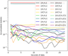Fig. A.1 Magnitudes of various cumulative statistics of data recorded with the MWA Voltage Capture System (Tremblay et al. 2015) at two neighboring tiles. All except the auto-correlations 〈|X|2〉 = 〈X*X〉 converge rapidly to zero.

Appendix B Linking R to Active Reflection Coefficient and τ

The quantity R_X and R_Y are the realized noise resistance of the array such that the noise voltage per $\sqrt{\Delta f}$ across the input impedance of the LNA can be calculated using $v_{n,X}=\sqrt{4kT{R}_X}$, and thus the total power delivered per unit bandwidth is given by $$P_{del,\text{ext}}=\Re \left\{\frac{|v_{n,X}{|}^2}{Z_{{}_{LNA}}^{*}}\right\}.$$(B.1)

The key point is that all the complex signal paths taken by the noise signal to reach the summing junction that exists due to mutual coupling are completely captured in RX. Additionally, we can show that R_X can be calculated using already-established quantities such as τ_X and the active impedance $z_{actu,X}^{\text{'}}$ calculated from the active reflection coefficient.

The quantity τ derived in Ung (2020) is a ratio of the power delivered to the LNA input impedance due to the homogeneous sky to the available power (kT). Therefore, we can easily convert τX to RX and vice versa using $$R_X=\frac{{\tau }_X}{4\Re \left\{\frac{1}{Z_{LNA}^{*}}\right\}}.$$(B.2)

Alternatively, the active reflection coefficient of an antenna element in an array as defined in Belostotski et al. (2015) can be used to calculate R_X. The active reflection coefficient accounts for all the coupling signal paths and combines it into a single equivalent signal path.

Hence, the power for each equivalent branch can be calculated using $$P_{del,i}=\frac{4kT}{N}{\left|\frac{z_{\text{LNA}}\sqrt{\Re \left\{{Z^{\prime }}_{actv{i}^{\prime }}\right\}}}{Z_{\text{LNA}}+{Z^{\prime }}_{actv,i}}\right|}^2\Re \left\{\frac{1}{Z_{{}_{LNA}}^{*}}\right\},$$(B.3)

and thus $$R_X=\frac{1}{N}{\displaystyle \sum _{i=1}^N\left|\frac{Z_{\text{LNA}}}{Z_{\text{LNA}}+{Z^{\prime }}_{actv,i}}\right|}\Re \left\{{Z^{\prime }}_{actv,i}\right\},$$(B.4)

where N is the number of antenna elements and $z_{actv,i}^{\text{'}}$ is the active impedance for a given polarization obtained from the active reflection coefficient of the i-th element.

Figure B.1 shows R_X as a function of frequency calculated using three methods. Equations (B.2) and (B.4) yield the same quantity as equation (12).

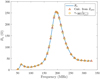Fig. B1 Comparison of Rx calculated using three methods. The solid curve was obtained using equation (12), while the data points represented by the circle and triangle markers are obtained using (B.2) and (B.4), respectively.

Appendix C Relation Between RMS Approximation and A/T

As demonstrated by Ung (2020), SEFD_XX/YY can be calculated using the realized area, Ar, and thus $$\begin{array}{l}{\text{SEFD}}_I^{rms}=\frac{1}{2}\sqrt{{\text{SEFD}}_{XX}^2+{\text{SEFD}}_{YY}^2}\hfill \\ =\frac{1}{2}k\sqrt{{\left(\frac{{\tau }_X{T}_{\text{sysX}}}{A_{rX}}\right)}^2+{\left(\frac{{\tau }_Y{T}_{\text{sysY}}}{A_{rY}}\right)}^2}\hfill \end{array}$$(C.1)

and $$A_r=\frac{{\eta }_0}{2}\frac{\Re \left\{Z_{\text{LNA}}\right\}}{|Z_{\text{LNA}}{|}^2}\Vert 1{\Vert }^2,$$(C.2)

where A_r can be interpreted as the area of the array such that for a given incident plane wave with power density, P_inc, the power delivered to the load is P_load = A_rP_inc. Alternatively, it can also be expressed as A_r = τA_e.

As demonstrated in Appendix B, the quantity τ relates to R. Substituting Eq. (C.2) and Eq. (B.2) into (C.1) and simplifying yields $${\text{SEFD}}_I^{rms}=\frac{4k}{{\eta }_0}\sqrt{\frac{T_{\text{sysX}}^2{R}_X^2}{\left|\right|1_X{\Vert }^4}+\frac{T_{\text{sysY}}^2{R}_Y^2}{\left|\right|1_Y{\Vert }^4}}.$$(C.3)

Appendix D Simulated and observed SEFD_XX and SEFD_YY

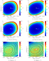Fig. D.1 Comparison of simulated and measured SEFDXX and SEFDYY. The relative difference MSEFD, in percent, is evaluated for each pixel.

References

All Tables

All Figures

Fig. 1 Arrays of dual-polarized low-frequency antennas observing the sky. The antennas are at fixed positions above the ground, and the z-axis is up. The signal from each element is amplified by an LNA, weighted, and summed. The output of each summation is directed into the correlator. The y-directed elements (black) follow the same signal flow, but are not shown. A four-element array is shown as an example.

In the text

	Fig. 2 Antenna length calculation for an array, where l1xθ is the antenna length associated with $\widehat{\theta }$ polarized incident field for x-directed antenna in the embedded element number 1 in the array shown, similarly to lixθ, liyθ, where i is the embedded element number. For brevity we consider a four-element array i = 1, ⋯, 4; the extension to i = 1, ⋯, N presents no complication.
In the text

	Fig. 3 Diagram representing system noise. The array is surrounded by a homogeneous blackbody radiator at temperature Tsys that represents the diffuse sky noise and the LNA noise. The y elements are similarly connected to a separate weight and summing circuit that are not shown for brevity.
In the text

	Fig. 4 Depiction of the vectors, their projections, and the area of the parallelogram.
In the text

Fig. 5 Example 0.5 s sky and difference images in X polarization (scale of the color bar is in Jy) used to calculate SEFD. Left: 0.5 s sky image. Center: difference between two consecutive 0.5 s images. Right: difference between two consecutive 0.5 s images corrected for the primary beam (divided by the primary beam in the X polarization). In order to calculate noise in every direction in the sky within the field of view (noise map), the standard deviation of the noise was calculated in small regions around each pixel in the difference image and divided by $\sqrt{2}$. These noise maps were later converted into SEFD using Eq. (29). The same procedure was applied to Y and is very similar to Stokes I polarizations (in this case the correction for the primary beam was more complex than the simple division by the corresponding primary beam).

In the text

	Fig. 6 SEFD in the pointing direction of gridpoint 114 with realized area calculated at (Az, ZA) = (80°, 46°) as a function of frequency. The observed SEFD calculated from calibrated visibilities is compared with simulated SEFD.
In the text

	Fig. 7 (a) Simulated SEFDI, (b) observed SEFDI, and (c) percentage difference between the simulated and observed SEFDI at 154.88 MHz calculated by Eq. (31).
In the text

	Fig. 8 Relative difference between the (a) simulated and (b) observed SEFDI and (c) the difference of $\Delta {\text{SEFD}}_I^{\text{obs}}$ and $\Delta {\text{SEFD}}_I^{\text{sim}}$
In the text

	Fig. 9 $\Delta {\text{SEFD}}_I^{\text{sim}}$ computed for 199.68 MHz at (Az, ZA) = (45°, 56.96°) showing the impact of the error resulting from the rms expression of SEFDI.
In the text

	Fig. A.1 Magnitudes of various cumulative statistics of data recorded with the MWA Voltage Capture System (Tremblay et al. 2015) at two neighboring tiles. All except the auto-correlations 〈|X|2〉 = 〈X*X〉 converge rapidly to zero.
In the text

	Fig. B1 Comparison of Rx calculated using three methods. The solid curve was obtained using equation (12), while the data points represented by the circle and triangle markers are obtained using (B.2) and (B.4), respectively.
In the text

	Fig. D.1 Comparison of simulated and measured SEFDXX and SEFDYY. The relative difference MSEFD, in percent, is evaluated for each pixel.
In the text

References

- Baudin, P. 2015, Wireless Transceiver Architecture: Bridging RF and Digital Communications, 1st edn. (Hoboken, NJ: Wiley) [Google Scholar]
- Belostotski, L., Veidt, B., Warnick, K.F., & Madanayake, A. 2015, IEEE Trans. Antennas Propag., 63, 2508 [CrossRef] [Google Scholar]
- Briggs, D.S. 1995, PhD thesis, The New Mexico Institute of Mining and Technology, USA [Google Scholar]
- Caiazzo, M. 2017, SKA Phase 1 System Requirements Specification V11, Technical Report SKA-TEL-SKO-0000008, SKA Organisation [Google Scholar]
- Chippendale, A.P., Hayman, D.B., & Hay, S.G. 2014, PASA, 31, e019 [NASA ADS] [CrossRef] [Google Scholar]
- Ellingson, S.W. 2011, IEEE Trans. Antennas Propag., 59, 1855 [CrossRef] [Google Scholar]
- Hillbrand, H., & Russer, P. 1976, IEEE Trans. Circuits Syst., 23, 235 [CrossRef] [Google Scholar]
- Labate, M.G., Braun, R., Dewdney, P., Waterson, M., & Wagg, J. 2017a, in 2017 XXXIInd General Assem. and Scientific Symp. of the Int. Union of Radio Sci. (URSI GASS), 1 [Google Scholar]
- Labate, M.G., Dewdney, P., Braun, R., Waterson, M., & Wagg, J. 2017b, in 2017 11th European Conference on Antennas and Propagation (EUCAP), 2259 [CrossRef] [Google Scholar]
- Lane, W.M., Cotton, W.D., van Velzen, S., et al. 2014, MNRAS, 440, 327 [NASA ADS] [CrossRef] [Google Scholar]
- McMullin, J.P., Waters, B., Schiebel, D., Young, W., & Golap, K. 2007, ASP Conf. Ser., 376, 127 [NASA ADS] [Google Scholar]
- Offringa, A.R., McKinley, B., Hurley-Walker, N., et al. 2014, MNRAS, 444, 606 [NASA ADS] [CrossRef] [Google Scholar]
- Offringa, A.R., Trott, C.M., Hurley-Walker, et al. 2016, MNRAS, 458, 1057 [NASA ADS] [CrossRef] [Google Scholar]
- Perley, R.A., & Butler, B.J. 2017, ApJS, 230, 7 [NASA ADS] [CrossRef] [Google Scholar]
- Sokolowski, M., Colegate, T., Sutinjo, A.T., et al. 2017, PASA, 34, e062 [NASA ADS] [CrossRef] [Google Scholar]
- Sokolowski, M., Jordan, C.H., Sleap, G., et al. 2020, PASA, 37, e021 [NASA ADS] [CrossRef] [Google Scholar]
- Strang, G. 2016, Introduction to Linear Algebra, 5th edn. (Wellesley, MA, USA: Wellesley-Cambridge Press) [Google Scholar]
- Sutinjo, A.T., Colegate, T.M., Wayth, R.B., et al. 2015, IEEE Trans. Antennas Propag., 63, 5433 [CrossRef] [Google Scholar]
- Sutinjo, A.T., Ung, D.C.X., & Juswardy, B. 2018, IEEE Trans. Antennas Propag, 66, 5511 [CrossRef] [Google Scholar]
- Sutinjo, A.T., Sokolowski, M., Kovaleva, M., et al. 2021, A&A, 646, A143 [NASA ADS] [CrossRef] [EDP Sciences] [Google Scholar]
- Thompson, A.R., Moran, J.M., & Swenson, G.W. 2017, Response of the Receiving System (Cham: Springer International Publishing), 207 [Google Scholar]
- Tingay, S.J., Goeke, R., Bowman, J.D., et al. 2013, PASA, 30, 7 [NASA ADS] [CrossRef] [Google Scholar]
- Tokarsky, P.L., Konovalenko, A.A., & Yerin, S.N. 2017, IEEE Trans. Antennas Propag., 65, 4636 [CrossRef] [Google Scholar]
- Tremblay, S.E., Ord, S.M., Bhat, N.D.R., et al. 2015, PASA, 32, e005 [CrossRef] [Google Scholar]
- Twiss, R.Q. 1955, J. Appl. Phys., 26, 599 [NASA ADS] [CrossRef] [Google Scholar]
- Ung, D.C.X. 2020, MPhil thesis, School of Electrical Engineering, Computing & Mathematical Sciences, Curtin University, Bentley, Western Australia [Google Scholar]
- Ung, D., Sutinjo, A., & Davidson, D. 2019a, in 2019 13th European Conference on Antennas and Propagation (EuCAP), 1 [Google Scholar]
- Ung, D., Sutinjo, A., Davidson, D., Johnston-Hollitt, M., & Tingay, S. 2019b, in 2019 IEEE International Symposium on Antennas and Propagation and USNC-URSI Radio Science Meeting, 401 [CrossRef] [Google Scholar]
- Ung, D.C.X., Sokolowski, M., Sutinjo, A.T., & Davidson, D.B. 2020, IEEE Trans. Antennas Propag., 68, 5395 [CrossRef] [Google Scholar]
- van Haarlem, M.P., Wise, M.W., Gunst, A.W., et al. 2013, A&A, 556, A2 [NASA ADS] [CrossRef] [EDP Sciences] [Google Scholar]
- Warnick, K.F., Woestenburg, B., Belostotski, L., & Russer, P. 2009, IEEE Trans. Antennas Propag., 57, 1634 [CrossRef] [Google Scholar]
- Warnick, K.F., Ivashina, M.V., Maaskant, R., & Woestenburg, B. 2010, IEEE Trans. Antennas Propag., 58, 2121 [CrossRef] [Google Scholar]
- Warnick, K.F., Ivashina, M.V., Wijnholds, S.J., & Maaskant, R. 2012, IEEE Trans. Antennas Propag., 60, 184 [CrossRef] [Google Scholar]
- Warnick, K.F., Maaskant, R., Ivashina, M.V., Davidson, D.B., & Jeffs, B.D. 2018, Phased Arrays for Radio Astronomy, Remote Sensing, and Satellite Communications, EuMA High Frequency Technologies Series (Cambridge: Cambridge University Press) [CrossRef] [Google Scholar]
- Wrobel, J.M., & Walker, R.C. 1999, ASP Conf. Ser., 180, 171 [NASA ADS] [Google Scholar]
The correlation products are in fact XX*, YY*, XY*, and YX*, but in the context of this section the conjugate symbols (*) were dropped for brevity.
MWA gridpoints are pointing directions where delays applied in the analog beamformers are exact.
All Tables
Calculated parameters required to compute SEFDI for the array pointing at the Hydra-A source (Az = 81°, ZA = 46°) on 2014-12-26 at 16:05:43 UTC.