| Issue |
A&A
Volume 660, April 2022
|
|
|---|---|---|
| Article Number | A132 | |
| Number of page(s) | 18 | |
| Section | Extragalactic astronomy | |
| DOI | https://doi.org/10.1051/0004-6361/202142523 | |
| Published online | 26 April 2022 | |
Stellar population gradients at cosmic noon as a constraint to the evolution of passive galaxies
1
Università degli studi di Milano-Bicocca, Piazza della scienza, 20125, Milano, Italy
e-mail: This email address is being protected from spambots. You need JavaScript enabled to view it.
2
INAF-Osservatorio Astronomico di Brera, via Brera 28, 20121 Milano, Italy
3
Carnegie Institution for Science, 813 Santa Barbara St., Pasadena, California 91101, USA
Received:
25
October
2021
Accepted:
26
January
2022
Abstract
Context. The radial variations of the stellar populations properties within passive galaxies at high redshift contain information about their assembly mechanisms, based on which galaxy formation and evolution scenarios may be distinguished.
Aims. The aim of this work is to give constraints on massive galaxy formation scenarios through one of the first analyses of age and metallicity gradients of the stellar populations in a sample of passive galaxies at z > 1.6 based on spectroscopic data from the Hubble Space Telescope.
Methods. We combined G141 deep slitless spectroscopic data and F160W photometric data of the spectroscopically passive galaxies at 1.6 < z < 2.4 with H160 < 22.0 in the field of view of the cluster JKCS 041. We extracted spectra from different zones of the galaxies, and we analysed them by fitting them with a library of synthetic templates of stellar population models to obtain estimates of the age and metallicity gradients.
Results. We obtained reliable measurements of age and metallicity parameters in different spatial zones of four galaxies. We performed spatially resolved measurements in individual high-redshift galaxies without the need of peculiar situations (i.e. gravitational lensing) for the first time. All four galaxies exhibit negative metallicity gradients. Their amplitude, similar to that measured in galaxies in the local Universe, suggests that the stellar populations of passive galaxies from z ∼ 2 to z = 0 are not redistributed.
Conclusions. Although the sample we analysed is small, the results we obtained suggest that the main mechanism that determines the spatial distribution of the stellar population properties within passive galaxies is constrained in the first 3 Gyr of the Universe. This is consistent with the revised monolithic scenario.
Key words: galaxies: clusters: individual: JKCS041 / galaxies: evolution / galaxies: high-redshift / galaxies: formation / galaxies: stellar content
© ESO 2022
1. Introduction
Understanding the formation and evolution of early-type galaxies (ETGs) is important because they contain almost 80% of the baryonic mass of the local Universe (Renzini 2006, and references therein). ETGs dominate the highest-density regions, such as clusters of galaxies (Dressler 1980, 1984; Balogh et al. 1999) up to z = 1.8 (Raichoor & Andreon 2012; Andreon et al. 2014; Strazzullo et al. 2019; Willis et al. 2020). In local clusters, ETGs are mainly elliptical and spheroidal galaxies, and they are populated by almost coeval old stars that apparently descended from a single star formation episode that occurred at z > 2 − 3 (e.g., Thomas et al. 2010). In the past decade, deep-field and cluster photometric surveys (e.g., Kurk et al. 2009; Van Dokkum et al. 2010; Papovich et al. 2010; Croom et al. 2012; Cassata et al. 2013; Straatman et al. 2014) and spectroscopic studies (e.g., Kriek et al. 2009; Gobat et al. 2012; Van de Sande et al. 2013; Newman et al. 2014; Andreon et al. 2014; Morishita et al. 2019; Willis et al. 2020) observed massive and passive galaxies (M > 1011 M⊙) that were already in place at z ∼ 2 − 3, and their stars were old compared with the age of the Universe at these redshifts.
Although numerous samples of passive galaxies have been analysed in the past decade, the mechanisms that describe their formation and evolution are still unclear. In particular, the relative importance of the environment and the mass in the regulation of the formation and the evolution of the ETGs is still debated (e.g., Treu et al. 2003; Thomas et al. 2010; Raichoor & Andreon 2012; Feldmeier-Krause et al. 2021). In rich clusters, the environment can play an important role in the evolution of ETGs. Various processes can regulate the ETG life in dense environments, such as interactions of the galaxy with the intracluster medium (ICM; e.g., ram-pressure stripping; Gunn & Gott 1972; Fujita & Nagashima 1999), galaxy-cluster gravitational interactions (e.g., tidal interactions; Byrd & Valtonen 1990; Henriksen & Byrd 1996), and interactions between galaxies (e.g., mergers; Icke 1985; Bekki 1998).
Several theoretical scenarios have been proposed to describe ETG formation and assembly. In the hierarchical galaxy formation model (Cole et al. 1994; Baugh et al. 1996; Kauffmann 1996; Kauffmann & Charlot 1998), ETGs are formed through subsequent wet mergers of pre-existing small galaxies moving in the same potential well (Toomre & Toomre 1972; De Lucia et al. 2006). In clusters, the mass assembly takes place earlier than in the field, with a higher rate of mergers (e.g., Maulbetsch et al. 2007; De Lucia & Blaizot 2007). ETGs grow faster in clusters than in the field (Andreon 2018).
Alternatively, ETGs might assemble their mass at z > 2 − 3 through the merger of small substructures that move in a common potential well (Dekel et al. 2009) in the so-called revised monolithic scenario. An almost purely passive evolution is expected to follow the strong initial activity, and only weak episodes of star formation at z < 1 are foreseen, for example caused by the capture of small satellites (Katz & Gunn 1991; Kawata 2001; Kobayashi 2004; Merlin & Chiosi 2006).
In recent years, the inside-out growth model has become widely accepted. Supported by several simulations (e.g., Khochfar & Silk 2006; Hopkins et al. 2009; Wuyts et al. 2010; Naab et al. 2009; Bezanson et al. 2009) and by observations of ETGs at 1.0 < z < 2.5 with an effective radius that is 3 − 5 times smaller than the mean radius of the local ETGs with the same mass (e.g., Newman et al. 2012, 2014; Andreon et al. 2016; Strazzullo et al. 2019), the model assumes that passive galaxies assemble as compact spheroids through wet merger events at z > 4 − 5. At lower redshift, the spheroids undergo various dry mergers with low-mass objects, which increases their effective radius.
These scenarios can be distinguished through a spatially resolved analysis of the stellar populations properties within passive galaxies. While in the hierarchical scenario, flat profiles of stellar population properties are expected (Bekki & Shioya 1999; Naab et al. 2009), in the monolithic scenario, stellar populations are expected to be more metal rich in the core zone of the galaxies than in their outskirts. Moreover, stochastic gradients are expected at different redshift in the inside-out growth scenario, where the final gradient depends on the nature and time of the satellite accretion events. Therefore, different distributions of stellar population properties within passive galaxies indicate different formation and/or evolution processes. Moreover, measurements of age and metallicity gradients in high-redshift galaxies, that is, in an epoch closer to their formation, can provide more direct constraints on the assembly mechanisms predicted by the models described above.
Recent studies that have analysed several samples of massive ETGs at low redshift (e.g., Kelson et al. 2006; Spolaor et al. 2009, 2010; Koleva et al. 2011; Scott et al. 2009; Greene et al. 2015; Ferreras et al. 2019; Zibetti et al. 2020), in particular in the Coma and Fornax clusters (Mehlert et al. 2003; Sánchez-Blázquez et al. 2006; Bedregal et al. 2011, and references therein) found strong negative metallicity gradients. The situation is less clear for the age gradients. Some studies show mild or null age gradients, while other studies reported strong positive age gradients (e.g., Kuntschner et al. 2010; Zibetti et al. 2020). It is important to note that age gradients of only 1–2 Gyr in local ETGs are difficult to detect in stellar popoulations that are more than 10 Gyr old on average, while their impact on the observed spectrophotometric properties is thought to be much more evident at higher redshift.
The study of age and metallicity gradients of the stellar populations in passive galaxies at high redshift would overcome the difficulty of detecting small age differences in old stellar populations and would offer information on the star formation history (SFH) and the mass assembly of ETGs closer to their formation epoch. Moreover, the age-metallicity degeneracy is predominant at low redshift (Worthey et al. 1994). Studies of ETGs at high redshift are expected to be less affected by the age-metallicity degeneracy because age is constrained within a narrow range of values allowed by the young age of the Universe.
Only a few stellar age and metallicity gradient measurements have been made at high redshift so far, and they are almost all based on photometric colours (Guo et al. 2011; Gargiulo et al. 2012). Colour-based measurements cannot break the age-metallicity degeneracy, so that they need to assume a fixed age to derive metallicity gradients or a fixed metallicity to derive possible age gradients. As an exception, Jafariyazani et al. (2020) found a clear negative metallicity gradient in spectroscopic data of a lensed galaxy at z = 1.98 that was sufficient magnified to be spatially resolved by ground-based spectroscopy. The metallicity gradient was comparable to that of local ETGs. The authors did not detect an age gradient, however.
The scarcity of gradient measurements in ETGs at high redshift is due to the current instrumental limits. Galaxies at z ∼ 2 have an apparent size of about 0.5 arcsec and are extremely faint. Data at a spatial resolution of about 0.1″ cannot be easily obtained with ground-based telescopes. Moreover, many spectral features that would be useful for measuring the age and metallicity of stellar populations at z ∼ 2 are redshifted to infrared wavelengths. These wavelengths are strongly contaminated by our atmosphere.
In the past decade, the capabilities of the Hubble Space Telescope (HST) have enabled us to overcome some of these limitations. The HST and its Wide Field Camera 3 (WFC3) provide both photometric and spectroscopic observations with an effective spatial resolution of ∼0.13 arcseconds.
We present a study based on deep slitless grism spectroscopy obtained with WFC3 using the G141 grism. We perform a spatially resolved investigation of the age and metallicity of stellar populations in a small sample of z ∼ 2 galaxies for the first time.
The plan of the paper is as follows. In Sect. 2 we introduce our sample and the spectroscopic and photometric data. In Sect. 3 we describe the analysis we carried out to obtain a robust measurement of age and metallicity gradients. In Sect. 4 we present our results. In Sect. 5 we discuss the constraints on the age and metallicity gradients and compare them to the literature. In Sect. 6 we present our conclusions and describe possible future works and implications. Throughout, we adopt a standard ΛCDM cosmology with ΩM = 0.3, ΩΛ = 0.7, and H0 = 70 km s−1 Mpc−1. Magnitudes are in the AB system.
2. Data and sample selection
The main data we used are slitless spectroscopic data obtained with the G141 grism and photometric data obtained with the F160W filter of the WFC3 mounted at the HST. The target of the observations is the cluster JKCS 041 at z ∼ 1.8. Spectroscopic data were taken during three separate visits with three different orientations for a total integration time of 17 ks. These are among the deepest G141 grism observations taken so far, and they target a field with the largest known number of high-redshift passive galaxies. The G141 grism covers the wavelength range from 10 750 Å to 17 000 Å at a nominal spectral resolution of R = 130 with a dispersion of 46.5 Å/pix. Photometric data consist of 4.5 ks deep images of the cluster field of view in three different orientations, with a pixel scale of 0.13 arcsec/pix.
Available data are reduced and background-subtracted 2D G141 spectra and calibrated background-subtracted F160W images for each visit (see details in Newman et al. 2014). We extracted 1D spectra corresponding to different portions of galaxies from the reduced spectroscopic 2D data, thus obtaining three spectra for each visit and each galaxy: one of the inner zone, and two of the outer zone (on either side of the centre).
The parent sample consists of all the 11 spectroscopically passive galaxies at 1.6 < z < 2.4 with H160 < 22.0 in the field of view of the cluster. The targets were classified by Newman et al. (2014) on the basis of their integrated HST G141 spectra. Seven of the 11 selected galaxies belong to the z ∼ 1.8 rich cluster JKCS 041, while 2 of the other 4 are foreground (z ∼ 1.6) and 2 are background (z ∼ 2.4) galaxies. Figure 1 shows the F160W magnitude of the selected targets as a function of their effective radius. Magnitudes and effective radii were calculated by Newman et al. (2014), except for ID64, for which they were calculated by us (as detailed in Andreon et al. 2016). The effective surface brightnesses of the sample cover a wide range from 20 (for compact galaxies) to 24 (for less compact galaxies) mag arcsec−2. Moreover, the effective radii of 9 out of 11 galaxies are smaller than one arcsecond.
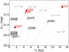 |
Fig. 1. H160 magnitudes vs effective radius of spectroscopic passive galaxies in the JKCS 041 field of view. Dashed lines indicate the locus of points with identical surface brightness within the effective radius in mag arcsec−2 (assuming the redshift of the cluster). The filled symbols indicate galaxies with constraints on metallicity and age gradients described in the text. The arrows indicate galaxies with an unknown effective radius. |
We discarded three galaxies (ID411, ID286, and ID376) from the sample a priori because their spectra were strongly contaminated or part of the spectra lay outside the detector limit. In the following section, we present the analysis of the remaining eight galaxies. As we explain in Sect. 4, we obtained reliable measurements of the age and metallicity parameters in different spatial zones for four out of eight galaxies.
3. Analysis
The main goal of our analysis is to constrain the ages and metallicities of the stellar populations in different zones of the considered galaxies. In this section, we compare synthetic templates and observed spectra in a small spectral window, extracted from different zones of the galaxies, and subsequently determine the corresponding stellar population parameters. We limit the following analysis to a very narrow spectral range in order to reduce the influence of the continuum on the determination of age and metallicity parameters. The shape of the spectral continuum is affected by λ-dependent dust extinction, and this can affect the age and metallicity estimates. Practically, the selected spectral ranges correspond to ∼4400 − 5300 Å rest frame for the foreground and cluster galaxies and to ∼3900 − 4500 Å rest frame for the background galaxies. These ranges contain spectral features that are sensitive to age and metallicity parameters in both cases.
3.1. Stellar population models
The galaxies in our sample were selected to be spectroscopically passive, and we adopted simple stellar population (SSP) models to represent their SFH with the aim of deriving the mean age and metallicity of their stellar population. Our reference analysis adopted the spectrophotometric SSP models by Bruzual & Charlot (2003) combined with the Chabrier (2003) IMF to build a synthetic spectral library. The BC03 models are based on the Padova tracks and isochrones combined with the MILES (Sánchez-Blázquez et al. 2007) empirical stellar library. These synthetic spectra cover the range in age from 0.4 Gyr to the lookback time between the galaxy redshift and zf = 6, and in metallicity from 0.02 Z⊙ to 2.5 Z⊙. We considered SSP because previous measurements in Newman et al. (2014) performed on our sample showed a best-fit timescale of exponentially declining SFHs of < 0.1 Gyr, as expected given the age of the Universe at high redshift and the passive nature of the sample. Any extended SFH therefore has by necessity a very short star formation timescale, which in turn makes them indistinguishable from data of our quality from SSP with slightly different ages (Longhetti et al. 2005). Nevertheless, we also considered other templates with different parameters and extended SFHs to demonstrate the robustness of our measurements (see Sect. 5).
3.2. Degradation of the synthetic spectra
Before they are compared with observations, synthetic spectra need to be: redshifted to the galaxy reference frame, degraded to the spectral resolution of the observed spectra (the spectral resolution is given by the combination of the nominal resolution of the instrument with the shape of the light profile along the dimension of the spectrum extraction), and rebinned to the pixel scale of the observed spectra. For numerical convenience (the galaxy radial profile is poorly known below the pixel resolution), we inverted the order of the last two processes in the analysis. We tested that this choice did not affect the final result by considering the worst-case scenario, which is an unresolved source with a Gaussian spectral feature comparable to the resolution of the observed spectra. For the second process, the kernel that was used to degrade the theoretical templates was derived by convolving the galaxy light profile with the nominal resolution of the instrument.
It is highly important to use the light profile of the galaxy to build the kernel because different galaxy profiles cause a different effective spectral resolution. The correlation with morphology means that the spectral resolution decreases with increasing galaxy size (morphological broadening; Van Dokkum et al. 2011). At the resolution of our data, the broadening caused by the galaxy extent is the dominant effect, corresponding to ∼2000 km s−1 rest-frame, and the dynamical motions within the galaxy can be ignored.
In order to measure the stellar population properties in different zones within the galaxies and to derive their gradients, we divided each galaxy into three zones and separately extracted the corresponding spectra from each G141 visit. We used the F160W image to extract the light profile of the galaxies corresponding to each of the extracted spectra because it matches the spectral coverage of the G141 grism. The extraction zones are larger in the outer than in the inner zone in order to partially compensate for the fact that the signal-to-noise ratio (S/N) is lower in the outskirts of the galaxies than in the central zones.
For each of the extraction zones, we derived the corresponding kernel function by convolving the light profile of the galaxy with a Gaussian with σ = 46.5 Å, representing the instrumental resolution of G141 grism. The resulting kernels were used to convolve the synthetic templates.
Figure 2 shows an example of the process described above. It was used to obtain the convolution kernel for a single visit of galaxy ID355. The left panel shows the division of the galaxy into three zones, corresponding to the extraction zones of the spectra. The upper right panel shows the three light profiles obtained by summing the pixels along the dispersion direction. The lower right panel shows the kernels obtained by convolving the light profile with the spectral resolution of the G141 grism. The outer kernels are broader and flatter than the inner kernel because the selected outer zones are spatially larger and fainter than the inner zone. Therefore the spectral features are broader in the outer zones than the inner zone.
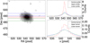 |
Fig. 2. Example of the process to obtain the convolution kernel for a single visit of the galaxy ID355. Left panel: F160W image of ID355 (single visit). Upper right panel: light profile of ID355. Each pixel along the dispersion side is 0.121 arcseconds wide, corresponding to 46.5 Å. Lower right panel: convolution kernel of ID355. |
Figure 3 shows an example of a synthetic spectrum redshifted to the ID355 reference frame and the same synthetic spectrum at the spectral resolution and binning of the observations. Despite the degradation of the spectrum, the absorption lines that are sensitive to the age and metallicity of the stellar populations (Hδ, Hγ, Hβ, and Mgb) are visible, suggesting that it is possible to measure the age and metallicity parameters at this spectral resolution.
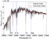 |
Fig. 3. Rebinning and convolution effects. In this example, we used a synthetic spectrum with solar metallicity and an age of 1 Gyr. The black line indicates the original redshifted spectrum, and the red line represents the rebinned and convolved spectrum. The vertical blue lines indicate the absorption lines we considered. |
3.3. Joint fit
Our statistical analysis was conducted with a Bayesian approach, which provides a powerful framework for inferring the age and metallicity of stellar populations in galaxies. Because the S/Ns of the observed spectra were low and diverse, we performed a joint fit of all the available data for each extraction zone in each galaxy. Upper and lower outer zones were considered together. The joint fit prevents the possible high noise of a single visit from degrading the signal coming from the other visits.
We compared the observed data with the redshifted, rebinned, and convolved synthetic templates within a narrow spectral range, and we computed the posterior probability of the age and metallicity parameters using the likelihood given by ℒ = e−χ2/2, where χ2 is
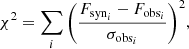 (1)
(1)
where Fsyn is the flux of the synthetic spectrum, and Fobs is the flux of the observed spectrum with the error σobs. The index i indicates the ith pixel on which the calculation takes place.
The total likelihood is given by the product of the likelihood of each visit. Before multiplying likelihoods, the observed spectra were inspected to determine possible contamination or cosmetic problems, such as reduction residuals or cosmic rays. The few spectra with p-values1 lower than 0.002 were discarded.
We assumed a uniform prior for age (from 0.4 Gyr to the lookback time between the galaxy redshift and zf = 6) because we considered only a small range, and a logarithmically uniform prior for metallicity (from 0.02 Z⊙ to 2.5 Z⊙), the latter following previous works (e.g., Gallazzi et al. 2014; Morishita et al. 2018; Zibetti et al. 2020). We explored the parameter space with a Markov chain Monte Carlo method (MCMC; Gilks 2005). The 68% probability interval is delimited by the 16° and 84° percentile. We also considered different prior distributions (uniform for metallicity, logarithmically uniform for age) to demonstrate the robustness of our measurements (see Sect. 5).
4. Results
As detailed in the previous paragraph, we extracted the spectra corresponding to the inner and outer zones of the eight galaxies introduced in Sect. 2. We measured the best fit and the joint probability distributions of the age and metallicity parameters in each zone for each of them. Sixty-eight percent of the posterior in four out of the eight galaxies (ID356, ID410, ID556, and ID628) is nearly equal to 68% of the assumed prior, and age and metallicity remain entirely unconstrained in at least one of the two zones (inner or outer), while for the remaining four galaxies (ID355, ID272, ID657, and ID64), the errors are smaller. Figure 4 shows the S/N in the outer zone as function of the S/N in the inner zone for the combined F160W image of all eight galaxies, and it suggests a way to preselect galaxies that are more likely to return useful constraints from a spectroscopic analysis without actually performing it. We calculated the photometric S/N using an aperture with a radius of two imaging pixels for the inner zone and a typical annulus with an inner radius of 4 pixels and an outer radius of 12 pixels for the outer zone. This matches the typical spectral apertures. Three galaxies (ID355, ID272, and ID64) are different from the remaining sample, in particular, they have a higher S/N in the outer zone. Galaxy ID657 represents a borderline case. It has one of the highest S/Ns in the inner zone and the best S/N in the outer zone of the other five galaxies. These four galaxies are characterised by the highest S/N in the outer regions (filled symbols) and are those for which our analysis obtained the smallest errors when we estimated age and metallicity in the two zones. Galaxies reported with empty circles represent galaxies for which the resulting age and metallicity estimates are affected by large errors, in particular in the outer zone, comparable to the prior we considered. For these galaxies, we cannot obtain information about their possible gradients even if it is present. The four galaxies for which we obtained the smallest errors therefore correspond to the galaxies with the highest S/N in the outer zone. This criterion could be used to find a priori suitable candidates in future surveys to study age and metallicity gradients without the need of performing a full spectroscopic analysis. Differences in the depths between the considered data need to be accounted for.
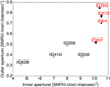 |
Fig. 4. F160W S/N of the inner and outer zones. The filled symbols indicate the galaxies described in the text. S/Ns are given for a single imaging pixel (0.06 × 0.06 arcsec2), but they were calculated as the average S/N over larger areas (∼10 for the inner zone, and ∼400 for the outer zone). |
In the following, we present our results for the four galaxies with the smallest errors (ID355, ID272, ID657, and ID64). They are also presented in Table 1. Three galaxies are members of JKCS 041, at z ∼ 1.8, and their fitted rest-frame wavelength range includes Hβ and Mgb features, which are sensitive to the age and metallicity of galaxy stellar populations, respectively. For the higher-redshift galaxy ID64, we considered the rest-frame range that includes Hδ and Hγ lines (sensitive to the stellar age) and G band (4300) (which is also sensitive to stellar metallicity).
Main characteristics of the four selected galaxies.
Figures 5 and 6 show the extracted spectra of galaxy ID355 and the corresponding best-fit templates in the inner and outer zone, respectively. Figure 7 shows the combined age and metallicity distributions obtained for ID355. Figures of the results obtained from the analysis of the other galaxies are shown in Appendix A.
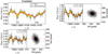 |
Fig. 5. Extracted spectra and the corresponding best-fit templates in the inner zone of galaxy ID355. Upper left panel: coadded spectrum of the inner zone of ID355 (line with errors) with the best-fit model in arbitrary units. Other panels: single-visit observed spectrum of the inner zone of ID355 with the best-fit model and the corresponding F160W images with the related extraction. |
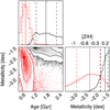 |
Fig. 7. Combined age and metallicity distributions obtained for ID355. Lower left panel: joint probability distribution of age and metallicity of the inner (black) and outer (red) zones of ID355. Contours are at 68% and 95% probability. Upper left panel: marginalised probability for the age. Lower right panel: marginalised probability for the metallicity. Median and 16% and 84% intervals are indicated by solid and dashed lines, respectively. |
Figure 8 summarises our results for the four galaxies. It reports the median value of age and metallicity for each zone and their 68% probability intervals. We find solar and supersolar metallicities in the inner zones of all the galaxies and subsolar values in the outer zones, indicating negative metallicity gradients in all four galaxies. Three out of the four galaxies the inner and outer zone have comparable ages, while ID355 presents an older stellar population in the inner zone than in the outskirts.
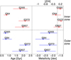 |
Fig. 8. Age (left panel) and metallicity (right panel) median values in the inner and outer zones of the sample. Solid lines show the 1σ errors. The vertical dashed line indicates solar metallicity. |
Finally, Fig. 9 shows the calculated median values of the age and metallicity gradients for the four galaxies. The gradients are defined as
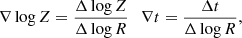 (2)
(2)
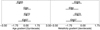 |
Fig. 9. Age (left panel) and metallicity (right panel) gradients of the sample. Solid lines show the 1σ errors. |
where log is the base-10 logarithm, Z is the metallicity, t is the age (Gyr), and Δlog R is the difference between the luminosity-weighted radius of the inner and outer extraction zones. Median values and errors are derived from the Bayesian probability density fuction of the gradients. Table 2 shows the median values of the marginalised posterior distribution of age and metallicity in the inner zone and their gradients. All four galaxies present negative metallicity gradients, even if their significance is only slightly above 1σ. Only one of the four galaxies, namely ID355, displays a negative age gradient. We obtained an average error of 0.7 dex/decade for the metallicity gradients and 0.6 Gyr/decade for the age gradients.
Median values of the marginalised posterior distribution of age and metallicity in the inner zone and their gradients.
Our gradient definition does not account for point spread function (PSF) effects, therefore the derived gradients underestimate the real gradients of the galaxies and should be handled with caution when compared with ground-based measurements with different (lower) spatial resolution. Moreover, the contamination of the spectra of the inner regions by the outer regions that lie along the dispersion direction might partially wash out the real gradients of the galaxies.
5. Discussion
We obtained reliable measurements of age and metallicity parameters in different spatial zones of four massive and spectroscopically passive galaxies. The entire sample exhibits negative metallicity gradients. Because of the very low spectral resolution combined with the low S/N that characterise our data, the 68% of the age posteriors in our analysis are of the order of 68% of the assumed prior (i.e. 16 − 84% percentile range). Our ability to detect possible age gradients in the galaxies exists only for age differences larger than the average value of 1.2 Gyr (see Fig. 9), to be compared with the mean age of their stellar content, ≈2 Gyr. A gradient like this has only been revealed in one of the four sample galaxies (ID355), while the other galaxies are consistent with a constant age with radius.
Before discussing the results, we verified whether they depend on the assumed model templates, on their selected parameters, or on the assumed priors. Moreover, in Appendix A, we show the robustness of our age and metallicity estimates by adding the effect of dust extinction as a further fitting parameter.
Figures 10 and 11 show the metallicity and age gradients, respectively, obtained in the reference case (i.e. based on the standard assumptions discussed in Sect. 3) and in test cases based on different assumptions listed in Table 3. The metallicity gradient estimates are very stable with respect to the possible model and prior assumptions. In particular, as expected, the results are unaffected by the assumption of a different age prior (logarithmically in place of linearly uniform), while for the assumption of a linearly uniform metallicity prior (in place of a logarithmically uniform prior), the stellar metallicity estimates move to higher values, as expected, but the corresponding gradients are consistent with those of the reference case. Different SFHs or formation redshift do not affect the resulting metallicity gradients at all. Figure 11 shows that age gradients are poorly constrained in the reference case, and the results obtained in any of the test cases are fully consistent with them. Results obtained considering templates that were derived from prolonged SFH models are not reported in this figure because the assumption of a prolonged initial star formation event corresponds to a smaller range of values of the age prior, and a direct comparison with the other cases is not possible. In Appendix B we show the joint age and metallicity probability distribution for the inner and outer zones of the sample that were obtained assuming a grid of templates derived from a top-hat SFH with a star formation timescale of 0.5 Gyr. Their comparison with those of the reference case shows that the only change in the results is a shift towards older ages of both zones. The limiting maximum age corresponding to the redshift of the galaxies flattens the resulting age gradients. Therefore, systematic errors are subdominant compared to statistical errors.
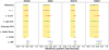 |
Fig. 10. Sensitivity analysis for the metallicity gradients. The reference analysis (black) adopts BC03 models, the MILES stellar library, a Chabrier IMF, and zf = 6. The result we obtained when we adopted a different zf = 11 is reported in violet, a different metallicity prior (uniform) in red, a different age prior (logaritmically uniform) in cyan, an extended star formation timescale (0.5 Gyr) in grey, a different stellar library (STELIB) in light blue, and a different model (Maraston) in brown. The blue, yellow, and green symbols are gradients derived by adopting a different IMF (−1.5 slope, Salpeter, and −3.5 slope, respectively). These slopes are systematically flatter because the range of metallicities considered in this comparison is smaller. |
Assumptions used for the sensitivity analysis.
To investigate the possible evolution of these galaxies, we now compare our results with those obtained at intermediate redshift and in the local Universe. In the local Universe, negative metallicity gradients are common within ETGs (e.g., Peletier et al. 1990; Idiart & Michard 2003; Scott et al. 2009; Zibetti et al. 2020). In particular, massive ETGs (M > 1010 M⊙; e.g., Mehlert et al. 2003; Ogando et al. 2005; Spolaor et al. 2009) show negative metallicity gradients up to −1.7 dex/decade. Figure 12 compares the age and metallicity parameters in the inner zone and their gradients as found in our high-redshift sample with the typical values obtained for massive ETGs in cluster environments in the local Universe (Mehlert et al. 2003). Mehlert et al. (2003) measured the radial variation up to 1Re of age and metallicity parameters for 35 ETGs in the Coma cluster. The good match of the metallicity estimates (within 1σ error) derived in two very distant cosmological epochs is remarkable and suggests that regardless of the evolution processes that occur in passive massive galaxies, the observed negative metallicity gradients must be kept from z ∼ 2 towards z = 0. A purely passive evolution is consistent with the ages estimated in the inner zones and with the corresponding gradients in the two samples, from z ∼ 2 towards z = 0, once the spread observed at z = 0 is accounted for. The Mehlert et al. (2003) age, metallicity, and gradients are highly consistent with the determination of Sánchez-Blázquez et al. (2006) for 37 ETGs in the Coma cluster. This confirms the soundness of our comparison sample.
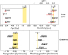 |
Fig. 12. Comparison between results for the local Universe (Mehlert et al. 2003) and our stellar age and metallicity parameters in the inner zone and their gradients. The arrow in the upper left panel indicates the lookback time between z = 0 and z = 1.8. The vertical dashed line indicates solar metallicity. |
Our results are also consistent with those obtained for a sample of quiescent field galaxies at z ∼ 0.8 (D’Eugenio et al. 2020), although a different environment was targeted. Because ground-based observations were used, D’Eugenio et al. (2020) were limited to analysing gradients on larger galaxy spatial scales than we probe.
To summarise, the negative metallicity gradients we found in the four high-redshift passive galaxies and their similarity with those retrieved in the local Universe suggest that the stellar populations of the passive galaxies are not redistributed over the last 10 Gyr. Our results support a scenario in which the main mechanism that determines the spatial distribution of the stellar population properties within passive galaxies is constrained in the first 3 Gyr of the Universe. This evidence can easily be explained within the revised monolithic scenario described in Sect. 1.
Our analysis, which is one of the first challenging attempts of measuring age and metallicity gradients in high-redshift galaxies, is surely limited by several factors: first of all, in the JKCS 041 field of view, we selected only the brightest and most massive three galaxies together with galaxy ID657 (Fig. 1). Althoug ID657 is fainter, it has the right combination of surface brightness and dimensions in order to be successfully analysed. Nonetheless, the three cluster galaxies span a representative range of parameters such as age, surface brightness, or stellar mass, considering that they are all galaxies with M > 1011 M⊙ (see Fig. 13). Moreover, the sample is small, therefore it is premature to extend our results to the entire class of passive galaxies at z ∼ 2. Nevertheless, it is unlikely (although not impossible) that the global negative metallicity gradients confirmed in all four galaxies are due to chance, indicating that they are probably a common feature in high-redshift passive galaxies.
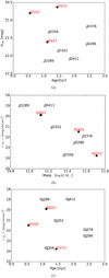 |
Fig. 13. Scale relations for cluster galaxies. Panel a: H160 magnitudes as a function of the ages of the quiescent galaxies of JKCS 041. Panel b: surface brightness within the effective radius as a function of the ages of the quiescent galaxies of JKCS 041. Panel c: surface brightness within the effective radius as a function of the mass of the quiescent galaxies of JKCS 041. Data are taken from Andreon et al. (2009). |
6. Conclusions
We presented the first estimates of the age and metallicity gradients based on spectroscopic data of a sample of 4 high-redshift (z ∼ 2) spectroscopically passive galaxies in the JKCS 041 field of view. The work is based on deep-grism slitless spectroscopic data taken with the G141 grism on HST/WFC3, which allowed us to spatially resolve starlight from galaxies with an apparent size of ∼1 arcsecond. The four galaxies for which the analysis was successful are part of a larger sample of 11 galaxies, 3 of which were immediately discarded due to their spectral contamination from other close objects within the field of view, while for the remaining four, the errors in age and metallicity were too large to derive any reliable conclusion. Alhtough the number of successufully analysed galaxies is small, they span quite wide ranges of values in Re and ⟨μe⟩, and they are only restricted in mass (M > 1011 M⊙).
The four galaxies for which the analysis was successful (ID355, ID272, ID657, and ID64) show negative metallicity gradients, although at only 1σ. Although the sample is small, the results we obtained and the comparison with metallicity and age gradients measured in the local Universe tend to support the revised monolithic scenario as the more probable paradigm for ETGs formation and evolution. We found metallicity gradients consistent with those confirmed at z = 0 and z = 0.8.
This work is the first study of stellar population properties gradients at high redshift based on spectroscopic data. It is therefore less limited by the age-metallicity degeneracy than the existing few works that are based on photometric data and colours (Guo et al. 2011; Gargiulo et al. 2012). Our analysis limits the effects of the possible presence of dust (selecting a narrow wavelength range for the analysis) and does not require the assumption of a particular age or metallicity to measure the variation of the other. Moreover, our analysis has the advantage of being applicable to a larger sample of galaxies than analyses that exploit unlikely events, such as the gravitational lensing produced by a massive cluster on the line of sight (Jafariyazani et al. 2020).
Despite the validity of the analysis we carried out, this work is subject to some limitations that are mainly due to the very low spectral resolution of the HST slitless data. Moreover, because of the low S/N, the analysed data allow the measurement of gradients that exceed a minimum threshold value (1.4 dex/decade for metallicity, 1.2 Gyr/decade for age), which limits the interpretation of the results in terms of galaxy formation scenarios. Despite the small sample size and the limitations affecting the analysis, the measurement of stellar population gradients in high-redshift galaxies using the HST grism has proven to be very promising in providing fundamental constraints on the galaxy formation scenarios. The analysis of larger samples, covering wider ranges of mass and sizes, is needed to derive a clear picture of the physical mechanisms that drive galaxy formation and evolution.
At the same time, our analysis has demonstrated the feasibility of an analysis like this even on the basis of very low spectroscopic resolution and at quite low S/N. This work has been successful not only in deriving the first reliable results, but also in tracing the way to identifying a set of spectroscopic data that is useful for this type of analysis.
The near future will offer many more opportunities through the advent of new facilities such as the James Webb Space Telescope, the Extremely Large Telescope and Euclid, which will provide not only the needed spatial resolution of about 0.1 arcsec, but also intermediate spectral resolution and even the possibility of obtaining 2D spectroscopic views of high-redshift galaxies. Future instruments will thus enable the study of stellar population property distributions in large samples of galaxies that also include less massive objects and cover a wide range of angular dimensions. This will open a new era in the study of galaxy formation and evolution.
The p-value is the probability of observing more extreme data under the assumption that the null hypothesis is correct.
Acknowledgments
We thank the anonymous referee for carefully reading the manuscript and for the stimulating suggestions that helped to improve the paper.
References
- Andreon, S. 2018, A&A, 617, A53 [NASA ADS] [CrossRef] [EDP Sciences] [Google Scholar]
- Andreon, S., Maughan, B., Trinchieri, G., & Kurk, J. 2009, A&A, 507, 147 [NASA ADS] [CrossRef] [EDP Sciences] [Google Scholar]
- Andreon, S., Newman, A., Trinchieri, G., et al. 2014, A&A, 565, A120 [NASA ADS] [CrossRef] [EDP Sciences] [Google Scholar]
- Andreon, S., Dong, H., & Raichoor, A. 2016, A&A, 593, A2 [NASA ADS] [CrossRef] [EDP Sciences] [Google Scholar]
- Balogh, M. L., Morris, S. L., Yee, H., Carlberg, R., & Ellingson, E. 1999, ApJ, 527, 54 [CrossRef] [Google Scholar]
- Baugh, C., Cole, S., & Frenk, C. 1996, MNRAS, 283, 1361 [NASA ADS] [CrossRef] [Google Scholar]
- Bedregal, A., Cardiel, N., Aragón-Salamanca, A., & Merrifield, M. 2011, MNRAS, 415, 2063 [NASA ADS] [CrossRef] [Google Scholar]
- Bekki, K. 1998, ApJ, 502, L133 [NASA ADS] [CrossRef] [Google Scholar]
- Bekki, K., & Shioya, Y. 1999, ApJ, 513, 108 [NASA ADS] [CrossRef] [Google Scholar]
- Bezanson, R., Van Dokkum, P. G., Tal, T., et al. 2009, ApJ, 697, 1290 [NASA ADS] [CrossRef] [Google Scholar]
- Bruzual, G., & Charlot, S. 2003, MNRAS, 344, 1000 [NASA ADS] [CrossRef] [Google Scholar]
- Byrd, G., & Valtonen, M. 1990, ApJ, 350, 89 [NASA ADS] [CrossRef] [Google Scholar]
- Calzetti, D., Armus, L., Bohlin, R. C., et al. 2000, ApJ, 533, 682 [NASA ADS] [CrossRef] [Google Scholar]
- Cassata, P., Giavalisco, M., Williams, C., et al. 2013, ApJ, 775, 106 [NASA ADS] [CrossRef] [Google Scholar]
- Chabrier, G. 2003, PASP, 115, 763 [Google Scholar]
- Cole, S., Aragon-Salamanca, A., Frenk, C. S., Navarro, J. F., & Zepf, S. E. 1994, MNRAS, 271, 781 [NASA ADS] [CrossRef] [Google Scholar]
- Croom, S. M., Lawrence, J. S., Bland-Hawthorn, J., et al. 2012, MNRAS, 421, 872 [NASA ADS] [Google Scholar]
- De Lucia, G., & Blaizot, J. 2007, MNRAS, 375, 2 [Google Scholar]
- De Lucia, G., Springel, V., White, S. D., Croton, D., & Kauffmann, G. 2006, MNRAS, 366, 499 [NASA ADS] [CrossRef] [Google Scholar]
- Dekel, A., Birnboim, Y., Engel, G., et al. 2009, Nature, 457, 451 [Google Scholar]
- D’Eugenio, F., van der Wel, A., Wu, P.-F., et al. 2020, MNRAS, 497, 389 [CrossRef] [Google Scholar]
- Dressler, A. 1980, ApJ, 236, 351 [Google Scholar]
- Dressler, A. 1984, ARA&A, 22, 185 [NASA ADS] [CrossRef] [Google Scholar]
- Feldmeier-Krause, A., Lonoce, I., & Freedman, W. L. 2021, ApJ, 923, 65 [NASA ADS] [CrossRef] [Google Scholar]
- Ferreras, I., Scott, N., La Barbera, F., et al. 2019, MNRAS, 489, 608 [Google Scholar]
- Fujita, Y., & Nagashima, M. 1999, ApJ, 516, 619 [NASA ADS] [CrossRef] [Google Scholar]
- Gallazzi, A., Bell, E. F., Zibetti, S., Brinchmann, J., & Kelson, D. D. 2014, ApJ, 788, 72 [Google Scholar]
- Gargiulo, A., Saracco, P., Longhetti, M., La Barbera, F., & Tamburri, S. 2012, MNRAS, 425, 2698 [NASA ADS] [CrossRef] [Google Scholar]
- Gilks, W. R. 2005, Encycl. Biostat., 4 [Google Scholar]
- Gobat, R., Strazzullo, V., Daddi, E., et al. 2012, ApJ, 759, L44 [Google Scholar]
- Greene, J. E., Janish, R., Ma, C.-P., et al. 2015, ApJ, 807, 11 [Google Scholar]
- Gunn, J. E., & Gott, J. R., III 1972, ApJ, 176, 1 [Google Scholar]
- Guo, Y., Giavalisco, M., Cassata, P., et al. 2011, ApJ, 735, 18 [NASA ADS] [CrossRef] [Google Scholar]
- Henriksen, M., & Byrd, G. 1996, ApJ, 459, 82 [NASA ADS] [CrossRef] [Google Scholar]
- Hopkins, P. F., Bundy, K., Murray, N., et al. 2009, MNRAS, 398, 898 [Google Scholar]
- Icke, V. 1985, A&A, 144, 115 [NASA ADS] [Google Scholar]
- Idiart, T., & Michard, R. 2003, A&A, 398, 949 [NASA ADS] [CrossRef] [EDP Sciences] [Google Scholar]
- Jafariyazani, M., Newman, A. B., Mobasher, B., et al. 2020, ApJ, 897, L42 [NASA ADS] [CrossRef] [Google Scholar]
- Katz, N., & Gunn, J. E. 1991, ApJ, 377, 365 [NASA ADS] [CrossRef] [Google Scholar]
- Kauffmann, G. 1996, MNRAS, 281, 487 [NASA ADS] [CrossRef] [Google Scholar]
- Kauffmann, G., & Charlot, S. 1998, MNRAS, 294, 705 [NASA ADS] [CrossRef] [Google Scholar]
- Kawata, D. 2001, ApJ, 548, 703 [NASA ADS] [CrossRef] [Google Scholar]
- Kelson, D. D., Illingworth, G. D., Franx, M., & Van Dokkum, P. 2006, ApJ, 653, 159 [NASA ADS] [CrossRef] [Google Scholar]
- Khochfar, S., & Silk, J. 2006, ApJ, 648, L21 [CrossRef] [Google Scholar]
- Kobayashi, C. 2004, MNRAS, 347, 740 [NASA ADS] [CrossRef] [Google Scholar]
- Koleva, M., Prugniel, P., De Rijcke, S., & Zeilinger, W. W. 2011, MNRAS, 417, 1643 [NASA ADS] [CrossRef] [Google Scholar]
- Kriek, M., Van Dokkum, P. G., Labbé, I., et al. 2009, ApJ, 700, 221 [NASA ADS] [CrossRef] [Google Scholar]
- Kuntschner, H., Emsellem, E., Bacon, R., et al. 2010, MNRAS, 408, 97 [Google Scholar]
- Kurk, J., Cimatti, A., Zamorani, G., et al. 2009, A&A, 504, 331 [NASA ADS] [CrossRef] [EDP Sciences] [Google Scholar]
- Longhetti, M., Saracco, P., Severgnini, P., et al. 2005, MNRAS, 361, 897 [NASA ADS] [CrossRef] [Google Scholar]
- Maulbetsch, C., Avila-Reese, V., Colín, P., et al. 2007, ApJ, 654, 53 [NASA ADS] [CrossRef] [Google Scholar]
- Mehlert, D., Thomas, D., Saglia, R., Bender, R., & Wegner, G. 2003, A&A, 407, 423 [NASA ADS] [CrossRef] [EDP Sciences] [Google Scholar]
- Merlin, E., & Chiosi, C. 2006, A&A, 457, 437 [NASA ADS] [CrossRef] [EDP Sciences] [Google Scholar]
- Morishita, T., Abramson, L., Treu, T., et al. 2018, ApJ, 856, L4 [NASA ADS] [CrossRef] [Google Scholar]
- Morishita, T., Abramson, L., Treu, T., et al. 2019, ApJ, 877, 141 [NASA ADS] [CrossRef] [Google Scholar]
- Naab, T., Johansson, P. H., & Ostriker, J. P. 2009, ApJ, 699, L178 [Google Scholar]
- Newman, A. B., Ellis, R. S., Bundy, K., & Treu, T. 2012, ApJ, 746, 162 [NASA ADS] [CrossRef] [Google Scholar]
- Newman, A. B., Ellis, R. S., Andreon, S., et al. 2014, ApJ, 788, 51 [NASA ADS] [CrossRef] [Google Scholar]
- Ogando, R. L., Maia, M. A., Chiappini, C., et al. 2005, ApJ, 632, L61 [NASA ADS] [CrossRef] [Google Scholar]
- Papovich, C., Momcheva, I., Willmer, C., et al. 2010, ApJ, 716, 1503 [NASA ADS] [CrossRef] [Google Scholar]
- Peletier, R. F., Davies, R. L., Illingworth, G. D., Davis, L. E., & Cawson, M. 1990, AJ, 100, 1091 [Google Scholar]
- Raichoor, A., & Andreon, S. 2012, A&A, 537, A88 [NASA ADS] [CrossRef] [EDP Sciences] [Google Scholar]
- Renzini, A. 2006, ARA&A, 44, 141 [NASA ADS] [CrossRef] [Google Scholar]
- Sánchez-Blázquez, P., Gorgas, J., & Cardiel, N. 2006, A&A, 457, 823 [NASA ADS] [CrossRef] [EDP Sciences] [Google Scholar]
- Sánchez-Blázquez, P., Forbes, D. A., Strader, J., Brodie, J., & Proctor, R. 2007, MNRAS, 377, 759 [Google Scholar]
- Scott, N., Cappellari, M., Davies, R. L., et al. 2009, MNRAS, 398, 1835 [NASA ADS] [CrossRef] [Google Scholar]
- Spolaor, M., Proctor, R. N., Forbes, D. A., & Couch, W. J. 2009, ApJ, 691, L138 [NASA ADS] [CrossRef] [Google Scholar]
- Spolaor, M., Kobayashi, C., Forbes, D. A., Couch, W. J., & Hau, G. K. 2010, MNRAS, 408, 272 [NASA ADS] [CrossRef] [Google Scholar]
- Straatman, C. M., Labbé, I., Spitler, L. R., et al. 2014, ApJ, 783, L14 [NASA ADS] [CrossRef] [Google Scholar]
- Strazzullo, V., Pannella, M., Mohr, J., et al. 2019, A&A, 622, A117 [NASA ADS] [CrossRef] [EDP Sciences] [Google Scholar]
- Thomas, D., Maraston, C., Schawinski, K., Sarzi, M., & Silk, J. 2010, MNRAS, 404, 1775 [NASA ADS] [Google Scholar]
- Toomre, A., & Toomre, J. 1972, ApJ, 178, 623 [Google Scholar]
- Treu, T., Ellis, R. S., Kneib, J.-P., et al. 2003, ApJ, 591, 53 [Google Scholar]
- Van de Sande, J., Kriek, M., Franx, M., et al. 2013, ApJ, 771, 85 [NASA ADS] [CrossRef] [Google Scholar]
- Van Dokkum, P. G., Whitaker, K. E., Brammer, G., et al. 2010, ApJ, 709, 1018 [NASA ADS] [CrossRef] [Google Scholar]
- Van Dokkum, P. G., Brammer, G., Fumagalli, M., et al. 2011, ApJ, 743, L15 [NASA ADS] [CrossRef] [Google Scholar]
- Willis, J., Canning, R., Noordeh, E., et al. 2020, Nature, 577, 39 [NASA ADS] [CrossRef] [Google Scholar]
- Worthey, G., Faber, S., Gonzalez, J. J., & Burstein, D. 1994, ApJS, 94, 687 [NASA ADS] [CrossRef] [Google Scholar]
- Wuyts, S., Cox, T. J., Hayward, C. C., et al. 2010, ApJ, 722, 1666 [NASA ADS] [CrossRef] [Google Scholar]
- Zibetti, S., Gallazzi, A. R., Hirschmann, M., et al. 2020, MNRAS, 491, 3562 [Google Scholar]
Appendix A: Fit and joint probability distributions
In this appendix we show the fit and joint probability distributions of the extracted spectra in the inner and outer zones for each galaxy. Figures from A.1 to A.6 show the fit results for the inner and outer zone of ID272, ID657, and ID64. Figures from A.7 to A.9 show the joint probability distributions for ID272, ID657, and ID64.
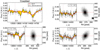 |
Fig. A.1. Extracted spectra and the corresponding best-fit templates in the inner zone of galaxy ID272. Upper left panel: Coadded spectrum of the inner zone of ID272 (line with errors) with the best-fit model in arbitrary units. Other panels: Single-visit observed spectrum of the inner zone of ID272 with the best-fit model and the corresponding F160W images with the related extraction. |
 |
Fig. A.7. Combined age and metallicity distributions obtained for ID272. Lower left panel: Joint probability distribution of age and metallicity of the inner (black) and outer (red) zones of ID272. Contours are at 68% and 95% probability. Upper left panel: Marginalised probability for age. Lower right panel: Marginalised probability for metallicity. Median and 16% and 84% intervals are indicated by solid and dashed lines, respectively. |
We verified whether the estimates of age and metallicity depend on dust attenuation AV assuming the Calzetti et al. (2000) law as a third parameter in the analysis. Considering the passive nature of our sample, we adopted values between 0 < AV < 0.7. Figures A.10 and A.11 show the comparison between marginalised probability distributions of age and metallicity, respectively, of the extracted spectra in the inner and outer zones for each galaxy in the case A(V) = 0 and 0 < A(V) < 0.7. These figures demonstrate that dust attenuation does not change the age and metallicity probability distribution for these galaxies appreciably.
 |
Fig. A.10. Comparison between the marginalised probability distribution of age in the case AV = 0 (solid lines) and 0 < AV < 0.7 (dashed lines) of the dust attenuation in the inner (black) and outer (red) zones for the four galaxies. |
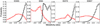 |
Fig. A.11. Same as Fig. A.10 for metallicity. |
Appendix B: Joint probability distributions with extended SFH
Even though the sampled galaxies were selected on the basis of their spectroscopic quiescency (i.e. τbest < 0.1 Gyr for exponentially declining SFHs) and their high redshift implies a very short star formation timescale, we performed the analysis assuming a top-hat SFH with a star formation timescale of 0.5 Gyr and 1.5 Gyr in order to access the dependence of the results on the SFH model assumptions. Figure B.1 shows the joint probability distributions for ID355, ID272, ID64, and ID657 in the reference case and with a top-hat SFH with a star formation timescale of 0.5 Gyr. The ages reported in the prolonged SFH case are mass-weighted mean ages. This figure demonstrates that a prolonged SFH does not change the metallicity probability distributions, while the age distributions are shifted to older ages, as expected. Regarding the more prolonged SFH (i.e. with a timescale of 1.5 Gyr), the corresponding templates do not fit the observed spectra at all (i.e. the  of the best-fitting model is larger than 3).
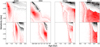 |
Fig. B.1. Comparison between the joint probability distribution of age and metallicity of the inner (black) and outer (red) zones in the reference case (upper panels) and with a top-hat SFH with a star formation timescale of 0.5 Gyr (lower panels) for the four galaxies. Contours are at 68% and 95% probability. |
All Tables
Median values of the marginalised posterior distribution of age and metallicity in the inner zone and their gradients.
All Figures
|
Fig. 1. H160 magnitudes vs effective radius of spectroscopic passive galaxies in the JKCS 041 field of view. Dashed lines indicate the locus of points with identical surface brightness within the effective radius in mag arcsec−2 (assuming the redshift of the cluster). The filled symbols indicate galaxies with constraints on metallicity and age gradients described in the text. The arrows indicate galaxies with an unknown effective radius. |
| In the text | |
|
Fig. 2. Example of the process to obtain the convolution kernel for a single visit of the galaxy ID355. Left panel: F160W image of ID355 (single visit). Upper right panel: light profile of ID355. Each pixel along the dispersion side is 0.121 arcseconds wide, corresponding to 46.5 Å. Lower right panel: convolution kernel of ID355. |
| In the text | |
|
Fig. 3. Rebinning and convolution effects. In this example, we used a synthetic spectrum with solar metallicity and an age of 1 Gyr. The black line indicates the original redshifted spectrum, and the red line represents the rebinned and convolved spectrum. The vertical blue lines indicate the absorption lines we considered. |
| In the text | |
|
Fig. 4. F160W S/N of the inner and outer zones. The filled symbols indicate the galaxies described in the text. S/Ns are given for a single imaging pixel (0.06 × 0.06 arcsec2), but they were calculated as the average S/N over larger areas (∼10 for the inner zone, and ∼400 for the outer zone). |
| In the text | |
|
Fig. 5. Extracted spectra and the corresponding best-fit templates in the inner zone of galaxy ID355. Upper left panel: coadded spectrum of the inner zone of ID355 (line with errors) with the best-fit model in arbitrary units. Other panels: single-visit observed spectrum of the inner zone of ID355 with the best-fit model and the corresponding F160W images with the related extraction. |
| In the text | |
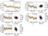 |
Fig. 6. Same as Fig. 5 for the outer zone of ID355. |
| In the text | |
|
Fig. 7. Combined age and metallicity distributions obtained for ID355. Lower left panel: joint probability distribution of age and metallicity of the inner (black) and outer (red) zones of ID355. Contours are at 68% and 95% probability. Upper left panel: marginalised probability for the age. Lower right panel: marginalised probability for the metallicity. Median and 16% and 84% intervals are indicated by solid and dashed lines, respectively. |
| In the text | |
|
Fig. 8. Age (left panel) and metallicity (right panel) median values in the inner and outer zones of the sample. Solid lines show the 1σ errors. The vertical dashed line indicates solar metallicity. |
| In the text | |
|
Fig. 9. Age (left panel) and metallicity (right panel) gradients of the sample. Solid lines show the 1σ errors. |
| In the text | |
|
Fig. 10. Sensitivity analysis for the metallicity gradients. The reference analysis (black) adopts BC03 models, the MILES stellar library, a Chabrier IMF, and zf = 6. The result we obtained when we adopted a different zf = 11 is reported in violet, a different metallicity prior (uniform) in red, a different age prior (logaritmically uniform) in cyan, an extended star formation timescale (0.5 Gyr) in grey, a different stellar library (STELIB) in light blue, and a different model (Maraston) in brown. The blue, yellow, and green symbols are gradients derived by adopting a different IMF (−1.5 slope, Salpeter, and −3.5 slope, respectively). These slopes are systematically flatter because the range of metallicities considered in this comparison is smaller. |
| In the text | |
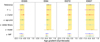 |
Fig. 11. Sensitivity analysis for the age gradients, colour-coded as in Fig. 10. |
| In the text | |
|
Fig. 12. Comparison between results for the local Universe (Mehlert et al. 2003) and our stellar age and metallicity parameters in the inner zone and their gradients. The arrow in the upper left panel indicates the lookback time between z = 0 and z = 1.8. The vertical dashed line indicates solar metallicity. |
| In the text | |
|
Fig. 13. Scale relations for cluster galaxies. Panel a: H160 magnitudes as a function of the ages of the quiescent galaxies of JKCS 041. Panel b: surface brightness within the effective radius as a function of the ages of the quiescent galaxies of JKCS 041. Panel c: surface brightness within the effective radius as a function of the mass of the quiescent galaxies of JKCS 041. Data are taken from Andreon et al. (2009). |
| In the text | |
|
Fig. A.1. Extracted spectra and the corresponding best-fit templates in the inner zone of galaxy ID272. Upper left panel: Coadded spectrum of the inner zone of ID272 (line with errors) with the best-fit model in arbitrary units. Other panels: Single-visit observed spectrum of the inner zone of ID272 with the best-fit model and the corresponding F160W images with the related extraction. |
| In the text | |
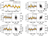 |
Fig. A.2. Same as Fig. A.1 for the outer zone of ID272. |
| In the text | |
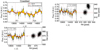 |
Fig. A.3. Same as Fig. A.1 for the inner zone of ID657. |
| In the text | |
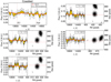 |
Fig. A.4. Same as Fig. A.1 for the outer zone of ID657. |
| In the text | |
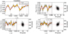 |
Fig. A.5. Same as Fig. A.1 for the inner zone of ID64. |
| In the text | |
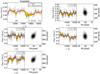 |
Fig. A.6. Same as Fig. A.1 for the outer zone of ID64. |
| In the text | |
|
Fig. A.7. Combined age and metallicity distributions obtained for ID272. Lower left panel: Joint probability distribution of age and metallicity of the inner (black) and outer (red) zones of ID272. Contours are at 68% and 95% probability. Upper left panel: Marginalised probability for age. Lower right panel: Marginalised probability for metallicity. Median and 16% and 84% intervals are indicated by solid and dashed lines, respectively. |
| In the text | |
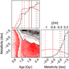 |
Fig. A.8. Same as Fig. A.7 for ID657. |
| In the text | |
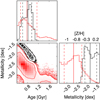 |
Fig. A.9. Same as Fig. A.7 for ID64. |
| In the text | |
|
Fig. A.10. Comparison between the marginalised probability distribution of age in the case AV = 0 (solid lines) and 0 < AV < 0.7 (dashed lines) of the dust attenuation in the inner (black) and outer (red) zones for the four galaxies. |
| In the text | |
|
Fig. A.11. Same as Fig. A.10 for metallicity. |
| In the text | |
|
Fig. B.1. Comparison between the joint probability distribution of age and metallicity of the inner (black) and outer (red) zones in the reference case (upper panels) and with a top-hat SFH with a star formation timescale of 0.5 Gyr (lower panels) for the four galaxies. Contours are at 68% and 95% probability. |
| In the text | |
Current usage metrics show cumulative count of Article Views (full-text article views including HTML views, PDF and ePub downloads, according to the available data) and Abstracts Views on Vision4Press platform.
Data correspond to usage on the plateform after 2015. The current usage metrics is available 48-96 hours after online publication and is updated daily on week days.
Initial download of the metrics may take a while.