| Issue |
A&A
Volume 660, April 2022
|
|
|---|---|---|
| Article Number | A121 | |
| Number of page(s) | 10 | |
| Section | Cosmology (including clusters of galaxies) | |
| DOI | https://doi.org/10.1051/0004-6361/202142296 | |
| Published online | 25 April 2022 | |
Missing large-angle correlations versus even-odd point-parity imbalance in the cosmic microwave background
1
Instituto de Física Corpuscular (IFIC) and Departamento de Física Teórica, Centro Mixto Universitat de València-CSIC, Dr. Moliner 50, 46100 Burjassot, Spain
e-mail: This email address is being protected from spambots. You need JavaScript enabled to view it.
2
Department of Physics, The Applied Math Program, and Department of Astronomy, The University of Arizona, Tucson, AZ 85721, USA
e-mail: This email address is being protected from spambots. You need JavaScript enabled to view it.
3
Instituto de Astrofísica de Canarias, 38205 La Laguna, Tenerife, Spain
e-mail: This email address is being protected from spambots. You need JavaScript enabled to view it.
4
Departamento de Astrofisica, Universidad de La Laguna, 38206 La Laguna, Tenerife, Spain
5
Departamento de Matemática da Universidade de Aveiro and Centre for Research and Development in Mathematics and Applications (CIDMA), Campus de Santiago, 3810-183 Aveiro, Portugal
Received:
24
September
2021
Accepted:
13
February
2022
Abstract
Context. The existence of a maximum correlation angle (θmax ≳ 60°) in the two-point angular temperature correlations of cosmic microwave background (CMB) radiation, measured by WMAP and Planck, stands in sharp contrast to the prediction of standard inflationary cosmology, in which the correlations should extend across the full sky (i.e., 180°). The introduction of a hard lower cutoff (kmin) in the primordial power spectrum, however, leads naturally to the existence of θmax. Among other cosmological anomalies detected in these data, an apparent dominance of odd-over-even parity multipoles has been seen in the angular power spectrum of the CMB. This feature, however, may simply be due to observational contamination in certain regions of the sky.
Aims. In attempting to provide a more detailed assessment of whether this odd-over-even asymmetry is intrinsic to the CMB, we therefore proceed in this paper, first, to examine whether this odd-even parity imbalance also manifests itself in the angular correlation function and, second, to examine in detail the interplay between the presence of θmax and this observed anomaly.
Methods. We employed several parity statistics and recalculated the angular correlation function for different values of the cutoff kmin in order to optimize the fit to the different Planck 2018 data.
Results. We find a phenomenological connection between these features in the data, concluding that both must be considered together in order to optimize the theoretical fit to the Planck 2018 data.
Conclusions. This outcome is independent of whether the parity imbalance is intrinsic to the CMB, but if it is, the odd-over-even asymmetry would clearly point to the emergence of new physics.
Key words: cosmological parameters / cosmic background radiation / cosmology: observations / cosmology: theory / inflation / large-scale structure of Universe
John Woodruff Simpson Fellow.
© ESO 2022
1. Introduction
As is well known, observations of the temperature fluctuations in the cosmic microwave background (CMB) radiation show that our Universe is quite uniform on scales much larger than the apparent (or Hubble) horizon (Melia 2018) at the time of decoupling. According to standard cosmology, this so-called horizon problem can be overcome by assuming an inflationary phase lasting a tiny fraction of a second almost immediately after the Big Bang (Starobinsky 1979; Kazanas 1980; Guth 1981; Linde 1982). Meanwhile, quantum fluctuations in the underlying inflaton field ϕ (Mukhanov 2005) would have grown and (somehow) classicalized to produce density perturbations that were also stretched enormously by the accelerated expansion, eventually forming the seeds of today’s large-scale structure, including galaxies and clusters (Peebles 1980). Inflation has also been invoked to explain why the Universe today appears to be spatially flat, if the initial spatial curvature was indeed set arbitrarily (but see Melia 2014). If this initial condition were truly indeterminate, the Universe would have required an astonishing degree of fine-tuning at the time of the Big Bang to evolve into what we see today without the effects of inflation.
The most popular inflation models tend to adopt the slow-roll condition, positing that the inflaton potential V(ϕ) changed very slowly during the phase of exponentiated expansion. For these scenarios, it is convenient to measure the inflation time as a function of the number of e-folds, Ne, in the expansion factor a(t). The duration of inflation would then be roughly equal to  , where Hϕ ≡ ȧ/a was the Hubble parameter at that time. In principle, the horizon and flatness problems might both be solved by requiring an inflation corresponding to Ne ≳ 60, one of the more notable successes of the inflation paradigm.
As we show below, however, the existence of a maximum correlation angle (θmax ≳ 60°) observed in the CMB by all three major satellite missions, COBE (Hinshaw et al. 1996), WMAP (Bennett et al. 2003), and Planck (Planck Collaboration VI 2018), implies a smaller number of e-folds (Ne ≈ 55), contrasting with most inflationary scenarios (Melia & López-Corredoira 2018; Liu & Melia 2020; Melia 2021). Moreover, this discrepancy does not stand in isolation. Many other puzzles and anomalies contributing to an increasing level of tension with standard cosmology (ΛCDM) have emerged in recent years as the accuracy of the observations has improved (see, e.g., the recent review by Perivolaropoulos & Skara 2021). For example, Schwarz et al. (2016) included in their list of CMB anomalies an apparent alignment of the lowest multipole moments with each other and with the motion and geometry of the Solar System, a hemispherical power asymmetry, and an unexpectedly large cold spot in the southern hemisphere. Di Valentino et al. (2021) argued against general concordance by demonstrating that a combined analysis of the CMB angular power spectrum obtained by Planck and the luminosity distance inferred simultaneously from type Ia supernovae (SNe) excludes a flat universe and a cosmological constant at the 99% confidence level. A broader view of the general tension between the predictions of ΛCDM and the observations may be found in López-Corredoira (2017). Whether some of these anomalies have a common origin becomes of paramount importance to the fundamental basis of our cosmological modeling.
In this paper we focus on two of the more recent discrepancies. The first is the lack of large-angle correlations seen in the CMB data, which seems to suggest that the primordial power spectrum, 𝒫(k), had a hard cutoff at a kmin distinctly different from zero. This explanation for the angular-correlation anomaly has recently been shown to also account self-consistently for the missing power at low ℓs in the angular power spectrum (Melia 2021). This feature in 𝒫(k) indicates the time at which inflation could have started (Liu & Melia 2020), hence setting an upper limit to the possible number of e-folds by the time it ended. It is kmin that now appears to create an inconsistency between the number of e-folds required to solve the horizon problem and that corresponding to the measured fluctuation spectrum (Melia & López-Corredoira 2018). The second is an apparent preference of the CMB data for an odd point-parity, first inferred from the analysis of the angular power spectrum (see, e.g., Kim et al. 2012; Schwarz et al. 2016). We seek to confirm whether this odd-even imbalance is also present in the measured angular correlation function, and if it is, we attempt to find a phenomenological connection between these two recently identified features in the CMB fluctuation distribution.
We note, however, that an interpretation of the odd-even imbalance as being intrinsic to the CMB anisotropies is not universally accepted. For example, Creswell & Naselsky (2021b) suggested that this asymmetry may be due to a contamination from a few regions of the sky. We return to this viable possibility toward the end of our discussion in Sect. 4. The work we carry out in this paper can therefore provide a more quantitative assessment of the idea that the an odd-even imbalance may originate within the CMB anisotropies for a more detailed comparison with the alternative scenario in which it is primarily due to some observational contamination. In doing so, we attempt to answer the questions whether (i) either one or the other of these characteristics is sufficient to account for the observed angular correlation function, or if are both required; and (ii) if the latter is true, whether the reoptimized value of kmin is different from that reported earlier (Melia & López-Corredoira 2018; Melia 2021) and might mitigate the current level of tension between the latest Planck release and the predictions of standard inflationary cosmology.
In this paper, we do not, however, include the potentially useful information concerning the polarization of the CMB radiation available from Planck for several practical reasons. The E-mode polarization arising from the Thomson scattering of photons by free electrons is dominated by optically thin plasma on small spatial scales. Therefore, these polarization effects cannot extend over large angular scales. In addition, the subtraction of foreground contamination is more difficult to carry out for polarized CMB light based on the current Planck data because of the required complex multicomponent fitting. Future missions such as Litebird (Errard et al. 2016), PICO (Hanany et al. 2019) and COrE (The COrE Collaboration 2011) will achieve more precise measurements at much higher sensitivity than is currently available with Planck, and should be able to answer the question of whether the large-angle anomalies seen in the temperature fluctuations are confirmed by the polarization maps.
2. Angular correlations in the CMB
One of the main goals of analyzing the angular correlation function of the CMB is to extract information regarding the different stages of the evolution of the Universe. Based on very general grounds, small (large) angles between CMB photon trajectories can be associated with small (large) length scales in the source plane (the opposite of using energy scales). Furthermore, it offers us the possibility of analyzing an important assumption in ΛCDM, that is, that the fluctuations are Gaussian and statistically homogeneous and isotropic. As previously noted, the angular correlation function of the CMB is already known to exhibit several statistical anomalies. In this section, we focus on the lack of large-angle correlations, but we first recall features in the CMB that are of special interest to this study.
It is customary to distinguish primary anisotropies arising prior to decoupling, from secondary anisotropies developed as the CMB photons propagate from the last scattering surface to the observer. We do not distinguish between recombination, last scattering surface, or freeze-out times, but approximate all of them as equal to a cosmic time td ≈ 3.8 × 10⁵ years (z ≃ 1100). For angles greater than a few degrees, the primary contributor to the former is the Sachs–Wolfe (SW) effect (Sachs & Wolfe 1967), representing fluctuations in the metric leading to temperature anisotropies via perturbations of the gravitational potential at the time of decoupling. There are two Sachs–Wolfe influences: the above-mentioned, nonintegrated Sachs–Wolfe effect, and the integrated Sachs–Wolfe effect (ISW). The latter is sometimes also further subdivided into an early ISW (taking place just after decoupling; for convenience, this is often just included in the SW), and a late ISW, arising while the CMB photons propagated through the expanding medium. The ISW contributes non-negligibly to the CMB anisotropies only if the universal expansion is at least partially driven by something other than purely nonrelativistic matter. In the standard model, dark energy – possibly in the form of a cosmological constant – started influencing the expansion at z ∼ 0.5, corresponding to a cosmic time ∼10 Gyr. The ISW has the effect of mainly raising the Sachs plateau at low multipoles. However, the detection of this ISW due to dark energy is not fully confirmed yet. The putative detections may simply be noise with underestimated error bars (López-Corredoira et al. 2010; Dong et al. 2021).
A way to address the angular dependence and anisotropies of the CMB is through its primary power spectrum, originally defined by the Fourier transform of the primordial fluctuation spectrum, usually parameterized as
![Mathematical equation: $$ \begin{aligned} \mathcal{P} (k)=A\ \biggl [\frac{k}{k_0}\biggr ]^{n_{\rm s}-1}, \end{aligned} $$](/articles/aa/full_html/2022/04/aa42296-21/aa42296-21-eq2.gif) (1)
(1)
where ns is the scalar spectral index. The spectrum would be perfectly scale free (with ns = 1) if the Hubble parameter Hϕ were strictly constant during inflation. In typical slow-roll inflationary models, however, this is only approximately true, and Hϕ evolves slowly, which produces a slight deviation of the spectral index from one. The observations show that in fact ns = 0.9649 ± 0.0042 (Planck Collaboration VI 2018), adding some observational support for a slow-roll potential, V(ϕ).
2.1. Two-point angular correlation function
The anisotropies in the CMB are very small, of about one part in 105, but they carry a wealth of information pertaining to the possible influence of V(ϕ) and the subsequent evolution of the Universe after reheating. A very powerful probe of these fluctuations is the two-point angular correlation function, defined as the ensemble product of the temperature differences with respect to the average temperature, from two directions in the sky defined by unitary vectors n1 and n2,
 (2)
(2)
The angle θ ∈ [0, π] is defined by the scalar product n1 ⋅ n2.
One typically expands C(θ) in terms of Legendre polynomials (assuming azimuthal symmetry)
 (3)
(3)
where the Cℓ coefficients encode the information with cosmological significance from the sky. The sum starts at ℓ = 2 and ends at a given ℓmax, dictated by the resolution of the data. The first two terms are excluded because (i) the monopole (ℓ = 0) is simply the average temperature over the whole sky and plays no role in the correlations, other than a global scale shift; and (ii) the dipole (ℓ = 1) is greatly affected by Earth’s motion, creating an anisotropy that dominates the intrinsic cosmological dipole signal.
2.2. Maximum angle in two-point angular correlations
Large-angle correlations in the CMB provide information about the earliest stages of the primitive Universe, well before recombination and the subsequent formation of cosmic structure. In this context, it may be useful to point out an interesting analogy with the angular correlations among the final-state particles in heavy-ion or proton-proton collisions at the Large Hadron Collider, and the early formation of nonconventional matter, such as a quark-gluon plasma or hidden valley particles (Sanchis-Lozano et al. 2020). In Fig. 1a we plot the observed angular correlation function (black dots) measured by Planck (Planck Collaboration VI 2018), compared with fitted (blue and red) curves to be discussed below. Above ≃60°, the correlations drop to near zero, except for a downward tail at ∼180°, which we also examine in more detail below. This shape of C(θ), particularly its suppression at large angles, was unexpected in standard cosmology, given that inflation was supposed to begin early enough (with kmin → 0) to provide the required number of e-folds to solve the horizon and flatness problems, thereby providing coverage across the full sky (see, e.g., Melia 2014).
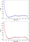 |
Fig. 1. Two-point correlation function C(θ) (solid curves) optimized to fit the Planck 2018 data (black points) (Planck Collaboration VI 2018). (a) Top panel: umin = 4.5 and odd-even parity balance of multipoles (blue curve). (b) Bottom panel: umin = 4.5 and odd-even parity dominance (red curve). See main text. |
It is worth mentioning at this point that these expectations on the value of kmin and correlations at all angles are primarily based on the correctness of the standard model. Large-angle correlations are not necessarily expected in all cosmological models, however. For example, in the alternative cosmology known as the Rh = ct universe, which does not have an inflationary epoch, the expansion factor is linear in time and the maximum angle corresponds to the size of the apparent horizon (Melia 2018) at decoupling,
 (4)
(4)
where td and t0 denote the decoupling and present cosmic times, respectively. The Rh = ct universe is an FLRW cosmology in which the equation of state is constrained by the zero active mass condition in general relativity, that is, ρ + 3p = 0. The Raychaudhuri equation clearly shows that ä = 0 in that case, which leads to a Universe expanding at a constant rate (Melia 2013a). This Universe has no horizon problem, and spatial flatness is ensured because the total energy density is zero. It therefore has no need for inflation. In such a universe, the Hubble parameter is always exactly equal to the inverse of the age of the Universe, and the Hubble radius satisfies Rh = ct at all times, hence the eponymous origin of its name. Setting td = 3.8 × 10⁵ years and t0 = 13.8 Gyr, we obtain θmax ∼ 40°. Thus, if inflation were to fail to adequately explain the existence of such a maximum correlation angle, it might be considered evidence supporting a noninflationary model, such as Rh = ct.
We generalize the expression in Eq. (4) by writing it in terms of the maximum fluctuation size λmax(td) at decoupling time td and the proper distance Rd ≡ a(td)rd (with rd the comoving distance) from us to the last scattering surface,
![Mathematical equation: $$ \begin{aligned} \theta _{\rm max}= 2 \tan ^{-1} \biggl [ \frac{\lambda _{\rm max}}{R_{\rm d}} \biggr ]. \end{aligned} $$](/articles/aa/full_html/2022/04/aa42296-21/aa42296-21-eq6.gif) (5)
(5)
Because we study the formation of primordial physical quantities, the apparent horizon (equal to the Hubble radius in this case) should set the basic length scale at stake (Melia 2013b, 2020b). In particular, the maximum fluctuation size can be estimated as λmax = α2πRh, where α ≲ 1 denotes a coefficient dependent on the cosmological model. For instance, α = 1 for de Sitter space and α ≃ 0.5 for ΛCDM (Melia 2013b, 2018). This scale changes as the expansion factor a(t) grows, starting with the assumed slow-roll inflation, followed by radiation and then matter-dominated evolution, before reaching decoupling, where the CMB radiation was released. Nevertheless, knowledge of Rh at decoupling is sufficient to estimate λmax associated with the largest fluctuation we can see in the CMB anisotropies today.
On the other hand, to compute the proper distance Rd between us and the last scattering surface, we must know the expansion history from decoupling to today. An excellent approximation for a(t) during this time may be written
 (6)
(6)
where  , with ΩΛ and H0 denoting the normalized dark matter density and Hubble constant today, respectively, and t the cosmic time since the Big Bang (see Appendix A).
In Fig. 2 we show the maximum correlation angle obtained in our study under different assumptions concerning the inflationary epoch. Figure 2a shows a 3D rendition of the maximum correlation angle as a function of cosmic time and the number of e-folds (Ne). The correlation angle remains confined to just a few degrees for any number of e-folds Ne ≲ 40. For Ne ≥ 62, on the other hand, the curve quickly reaches 180° along the whole cosmic time until now. For the sake of clarity, the maximum correlation angle evolution with cosmic time is shown in Fig. 2b for different Ne values, corresponding to vertical cuts in the 3D plot (Fig. 2a) (see Appendix A for the mathematical details).
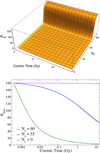 |
Fig. 2. Maximum correlation angle due to inflation. Top panel (a): 3D plot of the maximum correlation angle as a function of cosmic time and the number of e-folds. Bottom panel (b): maximum correlation angle evolution with cosmic time for different Ne values, corresponding to vertical sections in the 3D plot. We highlight that the plateau for Ne is smaller than about 50, implying a large inhomogeneity of the CMB along cosmic time. |
The late-time ISW effect yielding additional secondary anisotropies should tend to broaden the angular correlations as lower-ℓ multipoles are enhanced (due to a raising of the Sachs-plateau). Therefore, the number of e-folds required to comply with the observed maximum value of θmax should decrease even further once the ISW is taken into account. The Planck 2018 data therefore suggest that Ne ≲ 55, creating even greater tension with the conventional slow-roll inflationary scenario. Liu & Melia (2020) provided more details concerning the difficulties faced by the slow-roll paradigm to simultaneously solve the horizon problem and missing correlations at large angles.
Addressing these constraints from the latest CMB data would require a more complicated inflationary process than is usually conjectured. As we show below, this conclusion goes in the same direction as the need for a cutoff in the power spectrum in order to correctly reproduce the whole angular correlation function of the CMB.
2.3. Low cutoff in the CMB power spectrum
ΛCDM predicts an angular correlation curve that crosses the zero-axis twice and extends over the whole 180° range of poloidal angles (see, e.g., Fig. 1 in Melia 2014). This result is manifestly inconsistent with observational evidence, which shows a maximum correlation angle of ≥60°, as already discussed in the previous section.
In order to mitigate this tension, Melia & López-Corredoira (2018) introduced a cutoff to the primordial power spectrum, representing a lower limit to the integral
 (7)
(7)
where the normalization constant N and the minimum mode wavenumber kmin are optimized using a global fit to the whole observed angular correlation function. Although this procedure represents a phenomenological introduction of the cutoff kmin, this truncation has some theoretical justification in that it represents the first quantum fluctuation to either (i) have crossed the Hubble horizon once inflation started, or (ii) have emerged out of the Planck domain if inflation never happened (see Melia 2019; Liu & Melia 2020). The need for a kmin may also be related to the infrared regularization of the inflaton field commutator, although in standard cosmology, it should then likely be much smaller than its value (i.e., ≃3 × 10⁻⁴ Mpc−1, corresponding to umin = 4.34) optimized using the Planck 2018 data (Liu & Melia 2020).
In the computation of the Cℓ coefficients, only the SW effect is taken into account, ignoring other effects such as the baryon acoustic oscillations (BAO), whose influence extends primarily over smaller angles (θ ≲ 5°) and hence only the very large-ℓ multipoles (certainly > 100). Changing the integration variable from k to u ≡ krd in Eq. (7) and setting ns = 1 for simplicity, we obtain
 (8)
(8)
We point out that only those Cℓ coefficients with ℓ ≲ 20 are actually affected by the existence of the cutoff umin in the above integral.
In a previous computation of these coefficients using the Planck 2103 dataset, Melia & López-Corredoira (2018) found that the best fit to the angular correlation function is obtained with umin = 4.34 ± 0.50, which translates into a minimum wavenumber kmin = 4.34/r(td) (see also the similar limit placed on kmin by an analogous study of the angular power spectrum itself; Melia 2021). In the present paper, we repeated this analysis using the more recent Planck 2018 dataset, obtaining umin = 4.5 ± 0.5, and kmin = 4.5/r(td), which is compatible with the previous results from Planck 2013. We provide more details about the statistical analysis yielding this result below.
Very importantly, an almost zero correlation plateau above the maximum angle (θmax ≈ 60°) can be obtained by setting a lower cutoff to the integration variable u, corresponding to a lower cutoff in the power spectrum. Mathematically, this result can be understood as a delicate balance between even and odd multipole contributions to C(θ). We return to this crucial point in the next section.
3. Odd versus even point-parity in the CMB
Among the other anomalies observed in the CMB, an odd-even parity violation may indicate a nontrivial topology of the Universe, unexpected physics at the pre- or inflationary epochs, or some unsolved systematic errors in the data reduction. In the following, we focus on the apparent odd-dominance of the CMB fluctuations, that is, the fact that the weight of odd multipoles in either the power spectrum or the two-point angular correlation function is larger than the corresponding weight of the even multipoles. This imbalance is commonly referred to as a point-parity asymmetry of the CMB, and we address two statistics below that are widely employed to analyze it.
3.1. Odd-even parity statistics
We employ the parity statistic (Panda et al. 2021)
 (9)
(9)
where
 (10)
(10)
with the projectors defined as  and
and  . Assuming that ℓ(ℓ + 1)Cℓ is approximately constant at low ℓ, P± can clearly be considered as a measurement of the degree of parity asymmetry: below unity, it implies odd-parity dominance, and vice versa. Any deviation of this statistic from unity points to an odd-even parity imbalance.
A second statistic useful for checking a point-parity imbalance may be defined as the average ratio of the power in adjacent odd and even multipoles up to a given ℓ value (Aluri & Jain 2012; Panda et al. 2021),
 (11)
(11)
where  is the maximum odd multipole up to which the statistic is computed, and Dℓ ≡ ℓ(ℓ + 1)Cℓ/π. In contrast to P(ℓmax), the new statistic,
  , ensures that there are always the same number of odd and even powers along the whole considered multipole range, so no sawtooth oscillations are present. As for P(ℓmax), this statistic is also expected to fluctuate about the value of one at low ℓs.
In case of Gaussian fluctuations, the angular power spectrum and the angular correlation function contain the same information concerning the angular distribution of temperature in the CMB. Nevertheless, although the angular power spectrum covers all of the ℓ dependence, it emphasizes large-ℓ values, such that most of the information at θ ≳ 10° is squeezed into a very narrow interval, making it difficult to pick out any disagreement between theory and observation for the low multipoles. Conversely, the angular correlation function covers the fluctuation distribution more evenly over all angles, thereby making it relatively easier to study the large-angular region, corresponding to lower multipoles. Ultimately, both approaches should be mutually consistent as well as complementary for the extraction of useful information.
With this goal in mind, we require the statistic  (shown in red) to match (up to a given accuracy) the data (shown in black) in Fig. 3a. We do this by heuristically tuning the weights
 (12)
(12)
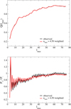 |
Fig. 3. Statistics used to describe the point-parity asymmetry of the CMB. (a) Top panel: |


to optimize the fit. Then, using the above ratios, we fit the two-point angular correlation function keeping two parameters free, namely, the normalization, N, and the cutoff kmin (i.e., umin). As noted earlier, the latter was already constrained to the interval umin ∈ (4.34 ± 0.50) in Melia & López-Corredoira (2018) using the old Planck 2013 data and without any consideration of a possible odd-even parity imbalance. We have carried out this analysis again for the latest Planck 2018 data at small, middle, and now large angles, incorporating the odd-parity dominance.
To incorporate these weights into the angular correlation function, we modified Eq. (3) to read
 (13)
(13)
with
 (14)
(14)
where ℓeven denotes even values of ℓ within the selected interval. The weights wℓ for the coefficients Cℓ, introduced ad hoc to model the odd-even imbalance, should not be confused with the window factors. Obviously, by requiring q(ℓeven)≡1 ∀ ℓeven, we obtain wℓeven = wℓeven + 1 = 1/2, thereby restoring the odd-even parity balance.
In Fig. 3a we show the function Q(ℓmax) for the Planck 2018 data (black) with the fit (red) corresponding to the set of parameters that provides the minimum reduced  for the angular two-point correlations, keeping the cutoff we introduced to improve the fit (see Table 1). The matching of the observed and theoretical values achieved by tuning the ratios q(ℓ) (and their respective weighting factors, wℓ) that modify the Cℓ coefficients is excellent. In addition, the set of weights optimized to find this match for Q(ℓmax) also produces an excellent fit in the P(ℓmax) plot, corresponding to a reduced
  near unity, as seen in Fig. 3b and Table 1.
 values for different fits to the two-point correlation function C(θ) and the parity statistic P(ℓmax), inferred from the Planck data. PB: parity balance; OD: odd dominance.
Figure 1b shows the plot of C(θ) over the whole range of angles with umin = 4.5, although this time, it incorporates the odd-dominance via the coefficients Cℓ, modified as explained above. The fit now also matches the downward tail at large angles. To understand what is happening, consider the separate plots in Fig. 4a that show the odd and even multipole contributions to C(θ). Each (odd and even) contribution behaves quite distinctly due to the intrinsic parity properties of the Legendre polynomials about θ = 90°. Consequently, once summed to produce the full C(θ), these two contributions produce constructive interference at small angles (i.e., θ < 90°) and destructive interference at large angles (θ > 90°).
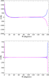 |
Fig. 4. Contributions from the even (blue) and odd (magenta) multipoles to the two-point angular correlation function C(θ) in Eq. (13) for (a) ℓ ∈ [2, 401] (top panel) and (b) ℓ ∈ [40, 401] (bottom panel). The delicate balance between odd and even polynomials is clear even at high ℓ for large angles. Selecting a different weighting of each contribution has a strong influence on C(θ) at θ ≃ 180°. |
One of our most important conclusions from this work is that in order to produce the optimum fit of the Planck 2018 data with the lowest  in Fig. 1b, we must include in our theoretical C(θ) both the cutoff umin in Eq. (8) and an odd-parity dominance via the weighting factors in Eq. (13). Otherwise, our fit to the observed data points for either the angular correlation function or the parity statistics worsens considerably, yielding a
  much larger than one. Using both the cutoff (kmin ≠ 0) and an odd-even parity imbalance simultaneously produces the best fit for C(θ), Q(ℓmax) and P(ℓmax) (see Table 1), however.
As noted earlier, we find from our study an optimized cutoff umin ≃ 4.5 ± 0.5, in which the mean value and σ = 0.5 error were obtained using a Monte Carlo analysis to sample the variation of C(θ) within the measurement errors. Since the C(θ) points are highly correlated, we circumvented this problem using a Monte Carlo procedure as described in Melia & López-Corredoira (2018). Starting from 100 mock CMB catalogs, we computed the two-point correlation function Ci(θ), (i = 1, 100) in each case. From these, we obtained ΔCi(θ) = Ci(θ)−C0(θ), where C0(θ) is the angular correlation function in standard cosmology. Then we calculated umin, i for C(θ) = CPlanck(θ)+ΔCi(θ) for each realization i. Next, from the resulting roughly Gaussian distribution of umin, i, we determined its average value and rms, yielding umin ≃ 4.5 ± 0.5, whose corresponding  distribution from the C(θ) fits varies smoothly around its minimum at 4.5. This umin range is slightly larger than but compatible with the interval obtained from the Planck 2013 dataset: umin = 4.34 ± 0.50.
A quantitative comparison of the various fits we have explored is provided in Table 1, which lists the  values for different choices of parameters, including the odd-even parity relative weights. A remark is in order: the improvement of the C(θ) fit, once umin = 4.5 is fixed, is somewhat modest when passing from parity balance to parity breaking. This is easy to understand because the main effect of imposing odd-dominance takes place at large angles, where the observational uncertainties are quite large and its impact on the total
  is thus relatively small. On the other hand, the agreement between the theoretical prediction and the parity statistic P(ℓmax) improves dramatically, as expected, given the observed odd-dominance, as seen in Fig. 3a.
We stress that the main benefit of using a kmin ≠ 0 together with parity breaking is not so much the improvement of the fit to the two-point correlations (with a focus on the tail at large angles) at the cost of increasing the number of degrees of freedom, but the fact that this approach can simultaneously resolve several apparently disconnected anomalies in the CMB. The end result is an excellent fit of C(θ) at small, medium, and large angles (reproducing the existence of a θmax ≳ 60°) with a p-value ≃0.95, and the implementation of an odd-parity dominance seen also in the angular power spectrum. This outcome constitutes the principal result of our analysis in this paper.
3.2. Relevance of the angular correlations at θ ≃ 180°
Large-angle correlations are commonly associated with low multipoles, typically ℓ ∈ [2, 20]. We have already established that the introduction of a cutoff kmin mainly affects multipoles with ℓ ≲ 20, and significantly alters the shape of the C(θ) curve at θ ≳ 60°. In contrast, the net contribution of multipoles with ℓ ≳ 20 practically cancels out, producing a plateau of zero correlation if nonuniform weights wℓ are excluded.
Nevertheless, the tail of C(θ) at θ ∼ 180° is influenced by the higher-order polynomials, even ℓ ≳ 20. To demonstrate this effect, we have split the angular correlation function into two pieces:
 (15)
(15)
The first piece, C(θ ; ℓ ≤ ℓ0), corresponds to the Cℓ coefficients that are significantly affected by umin in the integral of Eq. (8) and the different odd-even weighting factors used to produce Fig. 3a. The second summation runs from ℓ0 + 1 up to ℓup = 401 (ideally, infinity).
In contrast to conventional wisdom, the contribution of high-ℓ multipoles, C(θ ; ℓ ≥ ℓ0 + 1), can certainly influence C(θ) even at angles θ ∼ 180°. To see this, we separately plot in Fig. 4b the contributions of even and odd multipoles for ℓ0 > 40. Due to the oscillatory behavior of the Legendre polynomials, both contributions add to always produce a positive correlation at smaller angles, while a delicate balance exists at θ ∼ 180° that yields zero correlation when the parity symmetry is exact. A slight imbalance between odd and even high-ℓ multipoles, however, has a small (but observable) influence on the shape of the tail. We thus conclude that the value of C(θ ≃ 180° ) contains very interesting information concerning a possible odd-even parity imbalance even for high-ℓ multipoles.
4. Discussion
In spite of the high degree of isotropy in the CMB, certain anomalies have been found that create some tension with standard inflationary cosmology. The lack of long-range angular correlations beyond a maximum angle (θmax ≳ 60°) is difficult to reconcile with the basic inflationary paradigm, which is founded on the principle of a slow-roll potential producing an accelerated expansion of over 60 e-folds. This maximum correlation angle instead allows only about 55 e-folds, well below the number required to solve the temperature horizon problem. Moreover, as shown in Melia & López-Corredoira (2018), the feature (i.e., kmin) that maps into such a maximum correlation angle also produces a zero-correlation plateau in the two-point angular correlation function at all larger angles.
Meanwhile, it has been known for some time that the angular power spectrum of the CMB favours a weighting of odd multipoles over even (see, e.g., Kim et al. 2012). This anomaly could mean a breakdown of the odd-even parity expected in the cosmological principle, so its study carries great interest. In this paper, we therefore sought to determine whether these two features, that is, kmin and an odd-even parity imbalance, are related, and/or whether both are required to produce the best fit to the Planck 2018 data.
We have incorporated a possible odd-even parity imbalance in our analysis by introducing nonuniform weighting factors that modify the Cℓ coefficients in accordance with the parity statistic Q(ℓmax). The outcome of this analysis has resulted in an excellent fit to the two-point correlation function, including the tail associated with the odd-parity dominance at θ ∼ 180°. We have stressed that this angular region is influenced not only by the expected low-ℓ multipoles, but also to some degree by the high multipoles when the odd-even parity is broken.
At this stage, we can only speculate about a possible physical origin of kmin and/or an odd-even parity imbalance. Certainly, in the context of slow-roll inflation, the cutoff signals the time at which inflation could have started. This is the principal reason why a nonzero value of this truncation to the primordial power spectrum is so restrictive for the ability of inflation to solve the temperature horizon problem while simultaneously producing the distribution of anisotropies seen in the CMB. A natural question that arises in this context is whether the presence of a cutoff, kmin, should also impact the angular power spectrum itself. The answer appears to be yes, and it does so in a very intriguing way. It appears that the same value of umin required to optimize the fit to the angular correlation data also completely accounts for the ‘missing’ power seen in the low-multipole components (Melia 2021). The fact that the same feature in 𝒫(k), that is, a umin = 4.5 ± 0.5 (as we have found in this paper) can account for both empirically derived anomalies adds weight to its possible reality.
We here demonstrated that both kmin and an odd-even parity imbalance are required to optimize the fit to the Planck 2018 data, however. So what could be the origin of this parity violation? There is no known mechanism that can produce such an imbalance due to inflation on its own. Prior to classicalization, all of the quantum fluctuations seeded in the early Universe and expanded during inflation were spherically symmetric (Melia 2021). Suggestions have therefore tended to focus on possible nonstandard beginnings or trans-Planckian issues. For example, topological models involving multiconnected universes have been invoked to account for the anomalous cold spot, or the aforementioned missing power at low multipoles (Efstathiou 2003; Land & Magueijo 2006). Although these models can lower the power of the small-ℓ multipoles, they apparently cannot create an asymmetry, however.
At face value, an odd-even parity imbalance might be viewed as a possible trans-Planckian effect (Brandenberger & Martin 2013), given that this is the first instance following the Big Bang when features measurable today would have emerged into the semi-classical Universe (Melia 2020a). This topic touches on a broader issue related to the self-consistency of basic inflationary theory because the quantum fluctuations in the inflaton field would have been seeded in the so-called Bunch–Davies vacuum (Bunch & Davies 1978), well below the Planck scale. It is unclear, however, how or why quantum mechanics as we know it and general relativity could be used meaningfully to describe the evolution of these fluctuations on scales smaller than their Compton wavelength (see, e.g., Melia 2020a). In other words, an odd-even parity imbalance may turn out to be a signature of trans-Planckian physics once a viable theory of quantum gravity is devised, but there is no evidence of this right now. Any oscillatory and sharp features in 𝒫(k) tend to become completely smeared out by the time the CMB power spectrum is produced (Bennett et al. 2011). Other possibilities may also include bouncing cosmologies (Agullo et al. 2021).
If confirmed to be of cosmological origin, an odd-parity dominance would violate the Cosmological Principle. Together with the missing large-angle correlations, these two features could be an indication that new physics is required to modify the standard model accordingly, perhaps even leading to some exciting new discoveries about the origin and evolution of the Universe.
Regardless of its origin, however, the reality of an odd-over-even parity imbalance is becoming more firmly established in the analysis of the Planck data, making speculation such as this interesting to consider. Nevertheless, the existence of this asymmetry is by no means a certain indication that it originates from the CMB itself. As we indicated in the introduction, it may simply be due to an observational artifact. Recently, Creswell & Naselsky (2021b) discussed a link between the parity asymmetry and the low-ℓ peak anomaly, established in the presence of highly asymmetric regions in the sky, due to some foreground contamination in four regions near the Galactic plane ([ℓ,b]=[212° ,21° ], [32° ,21° ], [332° ,8° ], and [152° ,8° ]). This asymmetric distribution increases the odd-multipole power, while the deficit of symmetric regions leads to a corresponding deficit of even-multipole peaks. Therefore, the odd-even parity imbalance in the CMB could be explained, to a large statistical significance, as a consequence of an anomalous density of antipodal peaks in the sky once the dipole contribution from the motion of the Solar System is removed, without resorting to actual cosmological effects.
Having said that, we can safely conclude that our study in this paper establishes the compatibility of an infrared cutoff kmin in the power spectrum with an odd-over-even parity imbalance, regardless of its origin, either cosmological or due to contamination, or an incorrect foreground subtraction. Our analysis has shown that both kmin and the parity asymmetry are necessary in order to provide a best fit to the angular correlation function of the CMB.
5. Conclusion
This brief survey of possible causes of an odd-even parity imbalance is by no means exhaustive, but it is fair to conclude that a resolution of its origin will probably rely on new theoretical ideas. This stands in contrast to the meaning of kmin, which can indeed in some way be attributed to the inflaton potential, V(ϕ). At least theoretically, there would be no obvious connection between this cutoff and the odd-even parity imbalance. Nevertheless, the observational evidence suggests that both are necessary to optimize the fit to the Planck 2018 data, as hinted also for the WMAP observations by the earlier work reported in Kim et al. (2012), although the WMAP measurements had a lower precision than the Planck 2018 observations, and these authors did not analyze in depth the two-point angular correlation function over its whole angular range, as we have done here for Planck.
Our main conclusion is that neither the odd-even imbalance nor the cutoff kmin = 4.5/rd on their own and separately are sufficient to minimize the  of the C(θ) fit to the Planck 2018 data. Both are required, and while a nonzero kmin may be attributed to an as yet undiscovered inflaton potential, the odd-even imbalance would appear to signal entirely new physics, if it is not simply due to contamination.
Acknowledgments
This work has been partially supported by Agencia Estatal de Investigación del Ministerio de Ciencia e Innovación under grant PID2020-113334GB-I00/AEI/10.13039/501100011033, by Generalitat Valenciana under grant PROMETEO/2019/113 (EXPEDITE), by the Center for Research and Development in Mathematics and Applications (CIDMA) through the Portuguese Foundation for Science and Technology (FCT – Fundação para a Ciência e a Tecnologia), references UIDB/04106/2020 and UIDP/04106/2020, by national funds (OE), through FCT, I.P., in the scope of the framework contract foreseen in the numbers 4, 5 and 6 of the article 23, of the Decree-Law 57/2016, of August 29, changed by Law 57/2017, of July 19 and by the projects PTDC/FIS-OUT/28407/2017, CERN/FIS-PAR/0027/2019 and PTDC/FIS-AST/3041/2020. This work has further been supported by the European Union’s Horizon 2020 research and innovation (RISE) programme H2020-MSCA-RISE-2017 Grant No. FunFiCO-777740 and by FCT through Project No. UIDB/00099/2020.
References
- Abramowitz, M., & Stegun, I. A. 1970, Handbook of Mathematical Functions: with Formulas, Graphs, and Mathematical Tables (New York: Dover Books on Mathematics) [Google Scholar]
- Agullo, I., Kranas, D., & Sreenath, V. 2021, Class. Quant. Grav., 38, 065010 [NASA ADS] [CrossRef] [Google Scholar]
- Aluri, P. K., & Jain, P. 2012, MNRAS, 419, 3378 [NASA ADS] [CrossRef] [Google Scholar]
- Bennett, C. L., Hill, R. S., Hinshaw, G., et al. 2003, ApJS, 148, 97 [Google Scholar]
- Bennett, C. L., Hill, R. S., Hinshaw, G., et al. 2011, ApJ, 192, 17 [NASA ADS] [Google Scholar]
- Brandenberger, R. H., & Martin, J. 2013, Class. Quant. Grav., 30, 113001 [NASA ADS] [CrossRef] [Google Scholar]
- Bunch, T. S., & Davies, P. C. W. 1978, Proc. R. Soc. A, 360, 117 [NASA ADS] [Google Scholar]
- Creswell, J., & Naselsky, P. 2021a, J. Cosmol. Astropart. Phys., 2021, 103 [CrossRef] [Google Scholar]
- Creswell, J., & Naselsky, P. 2021b, ArXiv e-prints [arXiv:2105.08658] [Google Scholar]
- Di Valentino, E., Melchiorri, A., & Silk, J. 2021, ApJ, 908, L9 [NASA ADS] [CrossRef] [Google Scholar]
- Dong, F., Yu, Y., Zhang, J., Yang, X., & Zhang, P. 2021, MNRAS, 500, 3838 [Google Scholar]
- Efstathiou, G. 2003, MNRAS, 346, L26 [NASA ADS] [CrossRef] [Google Scholar]
- Errard, J., Feeney, S. M., Peiris, H. V., & Jaffe, A. H. 2016, J. Cosmol. Astropart. Phys., 2016, 052 [CrossRef] [Google Scholar]
- Guth, A. H. 1981, Phys. Rev. D, 23, 347 [Google Scholar]
- Hanany, S., Alvarez, M., Artis, E., et al. 2019, ArXiv e-prints [arXiv:1902.10541] [Google Scholar]
- Hinshaw, G., Branday, A. J., Bennett, C. L., et al. 1996, ApJ, 464, L25 [Google Scholar]
- Kazanas, D. 1980, ApJ, 241, L59 [Google Scholar]
- Kim, J., Naselsky, P., & Hansen, M. 2012, Adv. Astron., 2012, 960509 [CrossRef] [Google Scholar]
- Land, K., & Magueijo, J. 2006, MNRAS, 367, 1714 [NASA ADS] [CrossRef] [Google Scholar]
- Linde, A. D. 1982, Phys. Lett. B, 108, 389 [Google Scholar]
- Liu, J., & Melia, F. 2020, Proc. R. Soc. A, 476, 20200364 [NASA ADS] [CrossRef] [Google Scholar]
- López-Corredoira, M. 2017, Found. Phys., 47, 711 [CrossRef] [Google Scholar]
- López-Corredoira, M., Sylos Labini, F., & Betancort-Rijo, J. 2010, A&A, 513, A3 [NASA ADS] [CrossRef] [EDP Sciences] [Google Scholar]
- Melia, F. 2013a, A&A, 553, A76 [NASA ADS] [CrossRef] [EDP Sciences] [Google Scholar]
- Melia, F. 2013b, Class. Quant. Grav., 30, 155007 [NASA ADS] [CrossRef] [Google Scholar]
- Melia, F. 2014, A&A, 561, A80 [NASA ADS] [CrossRef] [EDP Sciences] [Google Scholar]
- Melia, F. 2018, Am. J. Phys., 86, 585 [NASA ADS] [CrossRef] [Google Scholar]
- Melia, F. 2019, Eur. Phys. J. C, 79, 455 [NASA ADS] [CrossRef] [Google Scholar]
- Melia, F. 2020a, Astron. Nachr., 341, 812 [NASA ADS] [CrossRef] [Google Scholar]
- Melia, F. 2020b, The Cosmic Spacetime (Oxford: Taylor& Francis) [CrossRef] [Google Scholar]
- Melia, F. 2021, Phys. Lett. B, 818, 136632 [Google Scholar]
- Melia, F. 2022, Astron. Nachr., 343 [CrossRef] [Google Scholar]
- Melia, F., & López-Corredoira, M. 2018, A&A, 610, A87 [NASA ADS] [CrossRef] [EDP Sciences] [Google Scholar]
- Melia, F., Ma, Q., Wei, J.-J., & Yu, B. 2021, A&A, 655, A70 [NASA ADS] [CrossRef] [EDP Sciences] [Google Scholar]
- Mukhanov, V. F. 2005, Physical Foundations of Cosmology (Cambridge: Cambridge University Press) [CrossRef] [Google Scholar]
- Panda, S., Aluri, P. K., Samal, P. K., & Rath, P. K. 2021, Astropart. Phys., 125, 102582 [erratum: Astropart. Phys., 130, 102582] [NASA ADS] [CrossRef] [Google Scholar]
- Peebles, P. J. E. 1980, The Large-Scale Structure of the Universe (Princeton: Princeton University Press) [Google Scholar]
- Perivolaropoulos, L., & Skara, F. 2021, ArXiv e-prints [arXiv:2105.05208] [Google Scholar]
- Planck Collaboration VI 2018, A&A, 641, A6 [Google Scholar]
- Sachs, R. K., & Wolfe, A. M. 1967, ApJ, 147, 73 [NASA ADS] [CrossRef] [Google Scholar]
- Sanchis-Lozano, M. A., Sarkisyan-Grinbaum, E. K., Domenech-Garret, J. L., & Sanchis-Gual, N. 2020, Phys. Rev. D, 102, 035013 [NASA ADS] [CrossRef] [Google Scholar]
- Starobinsky, A. A. 1979, J. Exp. Theor. Phys. Lett., 30, 682 [NASA ADS] [Google Scholar]
- Schwarz, D. J., Copi, C. J., Huterer, D., & Starkman, G. D. 2016, Class. Quant. Grav., 33, 184001 [NASA ADS] [CrossRef] [Google Scholar]
- The COrE Collaboration (Armitage-Caplan, C., et al.) 2011, ArXiv e-prints [arXiv:1102.2181] [Google Scholar]
Appendix A: Expansion factor following decoupling
The comoving distance to the last scattering surface may be written
 (A.1)
(A.1)
The scale factor a(t) determined from Friedmann’s equations for an isotropic and homogeneous Universe made of matter (dust) and dark energy reads
![Mathematical equation: $$ \begin{aligned} \biggl (\frac{\dot{a}}{a}\biggr )^2&=H_0^2\ \biggl [\frac{\Omega _m}{a(t)^3}+ \Omega _{\Lambda }\biggr ]\nonumber \\&\rightarrow a(t) \sim \biggl (\sinh \biggl [\frac{3}{2}\sqrt{\Omega _{\Lambda }} H_0t\biggr ]\biggr )^{2/3}\;, \end{aligned} $$](/articles/aa/full_html/2022/04/aa42296-21/aa42296-21-eq36.gif) (A.2)
(A.2)
where ΩΛ ≃ 0.7 and H0 denote the normalized dark matter density and Hubble parameter today, respectively. To simplify the notation, we define  , noting that in fact
  .
.
The proper (or physical) distance is given by
 (A.3)
(A.3)
so that
![Mathematical equation: $$ \begin{aligned} R_d=\ \sinh ^{2/3}{[\tilde{H}t_{d}]}\int _{t_d}^{t}\ \frac{dt^{\prime }}{\sinh ^{2/3}[\tilde{H}t^{\prime }]}\;. \end{aligned} $$](/articles/aa/full_html/2022/04/aa42296-21/aa42296-21-eq40.gif) (A.4)
(A.4)
Changing to the variable ![Mathematical equation: $ x=\sinh[\tilde{H}t] $](/articles/aa/full_html/2022/04/aa42296-21/aa42296-21-eq41.gif) , we obtain for the indefinite integral
, we obtain for the indefinite integral
![Mathematical equation: $$ \begin{aligned} \frac{1}{\tilde{H}}\ \int \ \frac{dx}{x^{2/3}(1+x^2)^{1/2}}=\frac{3\sinh ^{1/3}{x}}{\tilde{H}}\ _2F_1[1/2,1/6;7/6;-x^2]\;. \end{aligned} $$](/articles/aa/full_html/2022/04/aa42296-21/aa42296-21-eq42.gif) (A.5)
(A.5)
Next, invoking the basic property of the hypergeometric series (Abramowitz & Stegun 1970),
![Mathematical equation: $$ \begin{aligned} _2F_1[a,b;c;z]&= (1-z)^{-a}\ _2F_1[a,b-c;c;z/(z-1)]\ \rightarrow \nonumber \\ _2F_1[1/2,1/6;7/6;-x^2]&= \nonumber \\&\frac{1}{(1+x^2)^{1/2}}\ _2F_1[1/2,1;7/6;x^2/(1+x^2)]\;, \end{aligned} $$](/articles/aa/full_html/2022/04/aa42296-21/aa42296-21-eq43.gif) (A.6)
(A.6)
and reverting back to the original variable, we find the proper distance required to determine the maximum angle in Equation (5) to be
![Mathematical equation: $$ \begin{aligned} R_d&= \frac{3\sinh ^{2/3}[\tilde{H}t_{d}]}{\tilde{H}}\times \biggl (\frac{\sinh [\tilde{H}t]^{1/3}}{\cosh [\tilde{H}t]}\times \nonumber \\&\quad \quad _2F_1\biggl [1/2,1/6;7/6;\tanh ^2 [\tilde{H}t]\biggr ]- (t \rightarrow t_d)\biggr ), \end{aligned} $$](/articles/aa/full_html/2022/04/aa42296-21/aa42296-21-eq44.gif) (A.7)
(A.7)
where t here denotes the cosmic time of observation since the Big Bang. If the observation is today, then t = t0 is to be identified with the present age of the universe.
Appendix B: Error due to the finite cutoff ℓup
In this appendix, we estimate the accuracy of the Legendre expansion of C(π) over ℓup polynomials instead of infinity. For simplicity, we assume that the relation Cℓ = 2ℓ(ℓ+1) is satisfied for all ℓ; we therefore obtain 4πC(π) = 1/4, as defined in Equation (3) for all ℓ from 2 to ∞.
Thus, we may write
 (B.1)
(B.1)
This equation allows us to estimate the relative error made by neglecting polynomials of order higher than ℓup. In this work we set ℓup = 401, so that the relative error is about 0.5%. Other effects such as BAO at large ℓ have been neglected throughout this analysis because they have very little or no influence on the large angles we are focused on in this paper.
All Tables
values for different fits to the two-point correlation function C(θ) and the parity statistic P(ℓmax), inferred from the Planck data. PB: parity balance; OD: odd dominance.
All Figures
|
Fig. 1. Two-point correlation function C(θ) (solid curves) optimized to fit the Planck 2018 data (black points) (Planck Collaboration VI 2018). (a) Top panel: umin = 4.5 and odd-even parity balance of multipoles (blue curve). (b) Bottom panel: umin = 4.5 and odd-even parity dominance (red curve). See main text. |
| In the text | |
|
Fig. 2. Maximum correlation angle due to inflation. Top panel (a): 3D plot of the maximum correlation angle as a function of cosmic time and the number of e-folds. Bottom panel (b): maximum correlation angle evolution with cosmic time for different Ne values, corresponding to vertical sections in the 3D plot. We highlight that the plateau for Ne is smaller than about 50, implying a large inhomogeneity of the CMB along cosmic time. |
| In the text | |
|
Fig. 3. Statistics used to describe the point-parity asymmetry of the CMB. (a) Top panel: |
| In the text | |
|
Fig. 4. Contributions from the even (blue) and odd (magenta) multipoles to the two-point angular correlation function C(θ) in Eq. (13) for (a) ℓ ∈ [2, 401] (top panel) and (b) ℓ ∈ [40, 401] (bottom panel). The delicate balance between odd and even polynomials is clear even at high ℓ for large angles. Selecting a different weighting of each contribution has a strong influence on C(θ) at θ ≃ 180°. |
| In the text | |
Current usage metrics show cumulative count of Article Views (full-text article views including HTML views, PDF and ePub downloads, according to the available data) and Abstracts Views on Vision4Press platform.
Data correspond to usage on the plateform after 2015. The current usage metrics is available 48-96 hours after online publication and is updated daily on week days.
Initial download of the metrics may take a while.