Do the majority of stars form as gravitationally unbound?

František Dinnbier; Pavel Kroupa; Richard I. Anderson

doi:10.1051/0004-6361/202142082

Home

All issues

Volume 660 (April 2022)

A&A, 660 (2022) A61

Full HTML

Free Access

Issue		A&A Volume 660, April 2022


Article Number		A61
Number of page(s)		14
Section		Galactic structure, stellar clusters and populations
DOI		https://doi.org/10.1051/0004-6361/202142082
Published online		13 April 2022

A&A 660, A61 (2022)

Do the majority of stars form as gravitationally unbound?

František Dinnbier¹, Pavel Kroupa¹^,2 and Richard I. Anderson³

¹ Astronomical Institute, Faculty of Mathematics and Physics, Charles University, V Holešovičkách 2, 180 00 Praha 8, Czech Republic
e-mail: dinnbier@sirrah.troja.mff.cuni.cz
² Helmholtz-Institut für Strahlen- und Kernphysik, University of Bonn, Nussallee 14-16, 53115 Bonn, Germany
e-mail: pavel@astro.uni-bonn.de
³ Institute of Physics, Laboratory of Astrophysics, École Polytechnique Fédérale de Lausanne (EPFL), Observatoire de Sauverny, 1290 Versoix, Switzerland
e-mail: richard.anderson@epfl.ch

Received: 24 August 2021
Accepted: 6 January 2022

Abstract

Context. Some of the youngest stars (age ≲ 10 Myr) are clustered, while many others are observed scattered throughout star forming regions or in complete isolation. It has been intensively debated whether such scattered or isolated stars originate in star clusters or whether they form in truly isolated conditions. Exploring these scenarios could help set constraints on the conditions in which massive stars are formed.

Aims. We adopted the assumption that all stars form in gravitationally bound star clusters embedded in molecular cloud cores (Γ-1 model), which expel their natal gas early after their formation. Then we compared the proportion (fraction) of stars found in clusters with observational data.

Methods. The star clusters are modelled by the code NBODY6, which includes binary stars, stellar and circumbinary evolution, gas expulsion, and the external gravitational field of their host galaxy.

Results. We find that small changes in the assumptions in the current theoretical model estimating the fraction, Γ, of stars forming in embedded clusters have a large influence on the results, and we present a counterexample as an illustration. This calls into question theoretical arguments about Γ in embedded clusters and it suggests that there is no firm theoretical ground for low Γ in galaxies with lower star formation rates (SFRs). Instead, the assumption that all stars form in embedded clusters is in agreement with observational data for the youngest stars (age ≲ 10 Myr). In the Γ-1 scenario, the observed fraction of the youngest stars in clusters increases with the SFR only weakly; the increase is caused by the presence of more massive clusters in galaxies with higher SFRs, which release fewer stars to the field in proportion to their mass. The Γ-1 model yields a higher fraction of stars in clusters for older stars (ages between 10 Myr and 300 Myr) than what is observed. This discrepancy can be caused by initially less compact clusters or a slightly lower star-formation efficiency than originally assumed in the Γ-1 model, or by interactions of the post-gas-expulsion revirialised open clusters with molecular clouds.

Key words: galaxies: star formation / galaxies: stellar content / galaxies: star clusters: general

© ESO 2022

1. Introduction

Star formation takes place in the densest parts of molecular clouds. The youngest stars are usually found to be concentrated in embedded star clusters (Lada et al. 1991; Lada & Lada 2003; Megeath et al. 2016) or more dispersed throughout OB associations (Blaauw 1964). This opens two broad scenarios describing the plausible conditions for star formation.

In the first scenario, all stars form in gravitationally bound embedded clusters (e.g. Lada et al. 1984; Kroupa 1995a; Lada & Lada 2003; Porras et al. 2003; Kroupa et al. 2001; Banerjee & Kroupa 2017; González-Samaniego & Vazquez-Semadeni 2020), which form throughout a molecular cloud that, as a whole, might not be necessarily gravitationally bound but merely a condensation within the interstellar medium. The clusters expand and lose a substantial fraction of their stars as the result of the expulsion of the non-star-forming gas. The cores of some of these clusters survive the violent gas expulsion event (Lada et al. 1984; Boily & Kroupa 2003) and they are observed as gas-free open star clusters, while the escaping stars are receding out of clusters and are observed as unbound OB associations. After gas expulsion, the surviving cluster still evaporates and ejects stars, albeit at a slower rate than during gas expulsion. Dynamical ejections are particularly important for the most massive stars in the cluster, where the process is able to kick several tens of percent of OB stars from the cluster (Fujii & Portegies Zwart 2011; Oh et al. 2015; Oh & Kroupa 2016; Wang et al. 2019).

In the second scenario, stars form throughout the molecular cloud in hierarchical structures following the density field created by interstellar turbulence (e.g. Preibisch & Zinnecker 1999; Elmegreen 2000; Clark et al. 2005; Elmegreen et al. 2006). While some star formation occurs in initially bound clusters, a substantial proportion of star formation occurs in initially non-gravitationally bound groups. Thus, unlike in the first scenario, OB associations are gravitationally unbound from their formation.

In this context, it is useful to define the fraction of star formation Γ = CFR/SFR occurring in initially gravitationally bound embedded clusters. The CFR is the star formation rate within all bound clusters in the galaxy and the SFR is the total star formation rate of the galaxy.

The two scenarios have deep implications not only for the formation of bound star clusters, but also for massive star formation, which still lacks a full understanding (Zinnecker & Yorke 2007). In the first scenario, massive stars are clustered, and they compete for the available gas with each other (Bonnell et al. 1997, 2001), losing their specific angular momentum in the process, which naturally leads to their primordial mass segregation. In clusters, more massive stars can be also produced by mergers that are still in the pre-main-sequence stage (Bonnell et al. 1998). In contrast, the second scenario is based on massive star formation in isolation, for which there is not much observational evidence (Selier et al. 2011).

In the Galaxy, observations suggest that the majority (Γ = 0.5 to 1.0) of star formation occurs in embedded clusters (e.g. Carpenter et al. 1995; Carpenter 2000; Lada & Lada 2003; Porras et al. 2003; Bressert et al. 2010; Winston et al. 2020). An independent piece of evidence for Γ close to 1 comes from the observed lower binary fraction of field stars in contrast to the binary fraction in star forming regions, which can be explained as the result of dynamical processing within clusters (Kroupa 1995a,b; Marks & Kroupa 2011). When focusing on O stars, only 20% to 50% of them are located in the field (i.e. outside clusters or OB associations) (Mason et al. 1998), but many of the field O stars are unambiguously identified as runaway stars originating from bound systems (e.g. Blaauw 1964; Stone 1991; Tetzlaff et al. 2011; Gvaramadze et al. 2012), further decreasing the upper limit of truly isolated massive star formation.

In contrast, some observations of external galaxies point to a substantially lower values of Γ on the order of 0.1 (e.g. Goddard et al. 2010; Adamo et al. 2011; Johnson et al. 2016). Kruijssen (2012) suggests a semi-analytic model, according to which Γ increases with the star formation rate of the galaxy per unit area, Σ_SFR. However, Chandar et al. (2017) later found substantially larger values of Γ in galaxies with low Σ_SFR, and also no clear dependence of Γ on the Σ_SFR. These authors suggested that the dependency previously reported was caused by an age biased sample. Likewise, Fensch et al. (2019) reported large values for Γ in tidal dwarf galaxies located around the galaxy NGC 5291 that differ by ≈3σ from the estimate by Kruijssen (2012). Stephens et al. (2017) selected a sample of well-isolated massive young stellar objects in the Large Magellanic Cloud (LMC), previously thought to be massive stars formed in isolation, and found that each of them is surrounded by a star cluster of ≳100 stars, indicating that the vast majority (≳95%) of massive stars form in clusters, rather than in isolation. Thus, it is possible that the vast majority (if not all) massive stars found currently in isolation in external galaxies are, in reality, runaway stars or they are surrounded by a small star cluster consisting of lower-mass stars, which is not resolvable within the given survey.

In the present paper, we assume that all stars form in gravitationally bound embedded clusters (Γ = 1), which evolve as a result of their internal dynamics, gas expulsion, stellar evolution from a realistic initial stellar mass function (IMF), and the tidal field of their host galaxy. We study the proportion (fraction) of stars to be found within the clusters as a function of the cluster age, mass, and orbital radius within the galaxy, and we synthesise these results for a population of star clusters for a galaxy of a given global star formation rate in the framework of the integrated galactic initial mass function (IGIMF). Then we provide a comparison to observational data. Our assumption of Γ = 1 is in contrast to the theoretical value of ≈0.1, as expected for a Milky Way-like galaxy based on the theoretical model from Kruijssen (2012), which provides Γ as a function of the properties of the galaxy and favours isolated massive star formation in galaxies with lower star formation rates. We question some of the assumptions used in the theoretical model and we use a simple example to illustrate its main limitations.

2. Current model for Γ and its limitations

2.1. Overview of the model

Kruijssen (2012, hereafter K12) presented the first (and the only known to us) theoretical framework to infer Γ from the properties of the interstellar medium (ISM) of the particular galaxy. The model assumes that the probability density function dp/dx of the ISM mass density is log-normal and that star formation proceeds at a constant rate per free-fall time, so the denser gas produces stars more rapidly. The variable x denotes the normalised local density contrast, x = ρ/ρ_ISM, where ρ_ISM is the midplane density. Star formation is terminated either by gas exhaustion, by supernova feedback, or it still continues up to the age of interest. If star formation terminates by gas exhaustion, the final star formation efficiency (SFE ≡ stellar mass/(stellar plus gaseous mass)) is set to 0.5, which is motivated by the reduction of the stellar mass by protostellar outflows. If star formation is terminated by feedback from newly formed stars, the termination time is calculated by balancing the thermal pressure due to feedback with the turbulent pressure of the ISM.

The fraction of stars, γ, which form in gravitationally bound clusters is estimated to be linearly proportional to the SFE, namely, γ = 2 SFE (the factor of 2 is to reach γ = 1 for the maximum allowed SFE of 0.5). The clusters are subjected to tidal fields of passing interstellar clouds, which dissolve all clusters that had formed at a normalised density below x_cce on a timescale shorter than the specified age limit, which is chosen to be 10 Myr; clusters formed in gas above this density are assumed to be intact. Then, the fraction of stars which form in gravitationally bound clusters is calculated as:

$\begin{matrix} Γ = \frac{\int_{x_{cce}}^{\infty} γ (x) SFE (x) x (d p / d x) d x}{\int_{- \infty}^{\infty} SFE (x) x (d p / d x) d x} \cdot \end{matrix}$ $\begin{aligned} \Gamma = \frac{\int _{x_{\rm cce}}^{\infty } \gamma (x) \mathrm{SFE}(x) x (\mathrm{d} p/\mathrm{d} x) \mathrm{d} x}{\int _{-\infty }^{\infty } \mathrm{SFE}(x) x (\mathrm{d} p/\mathrm{d} x) \mathrm{d} x}\cdot \end{aligned}$ (1)

Since all the dependent variables under the integral sign, as well as x_cce, depend implicitly on the galactic parameters: Σ_g (mean gas surface density), Ω (angular frequency), and Q (Toomre parameter), Γ can be expressed as a function of these three galactic parameters. Further simplification is obtained by expressing the star formation rate, Σ_SFR, of the galaxy by Σ_g according to the Schmidt star formation law (Schmidt 1959; Kennicutt 1998). Taking typical values for the two other parameters (Ω and Q), K12 arrived at a formula for Γ as a function of Σ_SFR only. Because of this property, we refer to this model as the Γ − Σ_SFR model hereafter in this work.

2.2. Limitations of the model

The Γ − Σ_SFR model provides a valuable theoretical formulation for understanding the functional dependence of physical quantities. However, its derivation requires several simplifications or assumptions that require further consideration because they significantly affect model predictions. In particular:

What is probably the most significant simplification is the absence of the threshold for star formation of ≈120 M_⊙ pc⁻² (Lada et al. 2009, 2010; Heiderman et al. 2010), which suggests that star formation in the Galaxy is absent at gas densities below n(H₂)≈10⁴ cm⁻³ (≈300 M_⊙ pc⁻³). For the normalised density contrast, this means that star formation occurs only at x_lim ≳ 10⁴ (for a Milky Way-like galaxy), while the Γ − Σ_SFR model provides a much lower threshold of x_cce ≈ 10² for bound cluster formation and survival (Sect. 2.7.3 in K12). The model even considers scattered star formation at gas densities below x = 10² (cf. their Fig. 1), that is, at densities n(H₂)≲10² cm⁻³. The low star formation threshold results in many stars forming as gravitationally unbound, leading to low values of Γ.

The Γ − Σ_SFR model assumes (Sect. 2.5.2 in K12) that star formation proceeds at a constant rate until it is quenched by supernovae (occurring, at the earliest, 3 Myr after massive star formation started) or alternatively by radiation pressure. This neglects the influence of important early forms of stellar feedback, such as the photoionising radiation and stellar winds, which have a strong impact on the surrounding gas, substantially dispersing the natal cloud before the first supernova occurs (e.g. Rogers & Pittard 2013; Gavagnin et al. 2017; Haid et al. 2018; Dinnbier & Walch 2020). Neglecting early stellar feedback likely overestimates the value of SFE(x).

The functional form of the probability density function of self-gravitating star forming gas, which is a power-law function of a slope close to −2 (e.g. Kritsuk et al. 2011; Schneider et al. 2013; Lombardi et al. 2015; Chen et al. 2018) is very different from the log-normal distribution of non-self gravitating turbulent ISM (Vazquez-Semadeni 1994; Padoan et al. 1997; Kritsuk et al. 2011), as assumed in the Γ − Σ_SFR model.

As the collapse of the star forming cloud proceeds, its free-fall timescale decreases because density increases. Conversely, the Γ − Σ_SFR model assumes a constant SFR over time (Eq. (22) in K12).

To derive the density threshold x_cce (Sect. 2.7 in K12), it is assumed that the ISM velocity dispersion, σ_g, is constant regardless of the distance between the clumps. This is a reasonable approximation for the relative velocity between two molecular clouds. However, for the scale-free ISM within a given cloud, σ_g depends on distance, l, between the target cluster and the clump according to the Larson relations (e.g. Larson 1981; Heyer et al. 2009).

The Γ − Σ_SFR model assumes that all molecular clouds are of the same mass (Eq. (35) in K12).

The Γ − Σ_SFR model does not consider star cluster dynamics, which can eject a substantial fraction of young massive stars from clusters even during the first several Myr of the cluster’s existence (Perets & Šubr 2012; Oh et al. 2015; Wang et al. 2019), thus underestimating Γ.

Expulsion of the non-star forming gas is not considered here. Instead, it is assumed that most of the gas is consumed by star formation, which is not reproduced by many of the more recent star formation simulations (e.g. Colín et al. 2013; Gavagnin et al. 2017; González-Samaniego & Vazquez-Semadeni 2020).

In order to illustrate the strong dependence of the Γ − Σ_SFR model on the assumptions, we consider a very simple model for star formation that agrees with most observational facts, yet leads to completely different results than the Γ − Σ_SFR model. We stress that we use this as an illustration only and we do not intend to claim that star formation occurs according to this toy model. Rather, we argue that a radically different approach is needed to tackle the highly non-linear process of clustered star formation from a theoretical perspective. Considering that all stars form only at a density of x > x_lim and that star formation occurs in gravitationally bound clusters if x > x_cce, and in unbound associations if x < x_cce. It means that γ(x) = 1 for x > x_cce and 0 otherwise. We further assume that SFE(x) = 1/3 regardless of x (e.g. Geyer & Burkert 2001; Kroupa et al. 2001; Megeath et al. 2016; Banerjee & Kroupa 2017; Geen et al. 2018). From Eq. (1), these assumptions lead to Γ = 1 for galaxies with x_cce < x_lim, and Γ decreasing with x_cce for x_cce > x_lim, with x_cce = x_lim at log₁₀(ρ_ISM [g cm⁻³]) ≈ −21.8 (taking aside the weaker dependence on Ω and Q, we note that x_cce can be used as a proxy for Σ_SFR). This model stands in a stark contrast to the Γ − Σ_SFR model, where Γ ≈ 0.1 for galaxies with low x_cce of ≈ 10², which increases with x_cce towards ≈ 0.7.

By choosing different functional forms for γ(x) and SFE(x), neither of which are well constrained, it is easy to find an almost arbitrary dependence of Γ on x_cce and, therefore, on Σ_SFR. The extreme sensitivity on initial assumptions¹ is caused by recursively substituting equations for one another, several of which are non-linear or contain terms of uncertain importance. This behaviour is typical for chaotic systems, which cannot be understood by linearising or simplifying relevant equations. Thus, redoing the analysis for the Γ − Σ_SFR model in the same way will not yield more reliable results even if the aforementioned issues are resolved.

The above toy model illustrates that even minor changes in the assumptions of the Γ − Σ_SFR model lead to drastically different outcomes, thus challenging the previously suggested theoretical result stating that in a Milky Way-like galaxy, most stars form in gravitationally unbound entities.

In the following, we have therefore adopted the opposite approach, namely, based on the assumption that all stars form in gravitationally bound embedded clusters (i.e. Γ = 1), we investigate the currently observed fraction of bound stars by dynamical N-body simulations. The assumption of Γ = 1 is motivated by observational surveys of pre-main sequence stars in molecular clouds (e.g. Lada et al. 1991; Megeath et al. 2016; Joncour et al. 2018), the distribution functions of binary stars in the Galactic field in comparison to star forming regions (e.g. Reipurth & Zinnecker 1993; Leinert et al. 1993; Kroupa 1995b), and the general argument that a star forming molecular cloud core is observed to always contain significantly more gas than the weight of a single late-type star (Alves et al. 2007; Goodwin et al. 2008). We refer to the present model as the Γ-1 model to distinguish it from the Γ − Σ_SFR model.

Further assumptions of the Γ-1 model are that the clusters are initially compact (half-mass radii r_h of ≲1 pc for clusters of mass M_ecl ≲ 10⁴ M_⊙). The initial cluster mass function is a power-law (Eq. (4)), whose slope and upper mass limit follows from the galactic star formation rate, as obtained from IGIMF theory (Kroupa & Weidner 2003). The clusters form with SFE = 1/3, and they expel their non-star-forming gas on the timescale of r_h/10 km s⁻¹ ≈ 0.05 Myr at the cluster age of 0.6 Myr.

The particular values of the parameters in the Γ-1 model might be adjusted in the future when more accurate observational data become available. This iteration could provide another constraint on the birth properties of star clusters.

3. Model description and numerical method

3.1. Model description

The main results of this article are based on the models presented in Sect. 3.1.1 and correspond to the most probable initial conditions for embedded star clusters (standard models). To assess the dependence on the particular choice of initial assumptions, we compute additional models to investigate the influence of the initial cluster radius, the SFE, and primordial mass segregation (Sect. 3.1.2).

3.1.1. Standard models

Observed open clusters are well described by the Plummer model (e.g. Röser et al. 2011; Röser & Schilbach 2019) and star-forming molecular cloud filaments have Plummer-like cross-sections (e.g. André et al. 2014), which motivates us to use this description as initial conditions for present models. The Plummer model is described by its stellar mass, M_ecl, and Plummer parameter, a_ecl. The Plummer parameter is related to the cluster mass by the mass-radius relation of Marks & Kroupa (2012), where

$\begin{matrix} \frac{a_{ecl}}{pc} = 0.077 {(\frac{M_{ecl}}{M_{⊙}})}^{1 / 8} . \end{matrix}$ $\begin{aligned} \frac{a_{\rm ecl}}{\mathrm{pc}} = 0.077 \left(\frac{M_{\rm ecl}}{M_\odot }\right)^{1/8}. \end{aligned}$ (2)

The stellar masses of the clusters in our model grid are 50 M_⊙, 100 M_⊙, ...6400 M_⊙, which approximately covers the mass range of observed star clusters in the Galaxy and the galaxy M 31. To obtain better statistics, we simulate the 50 M_⊙ clusters 256 times with different random seeds, 100 M_⊙ clusters 128 times etc., so the 6400 M_⊙ clusters are simulated twice.

Stellar masses are sampled from the Kroupa (2001) model of the initial mass function (IMF) in the given mass range (0.08 M_⊙, m_max). To allow only the more massive clusters to form massive stars, we adopted the m_max − M_ecl relation from (Weidner et al. 2010; see also Elmegreen 1983, 2000 for earlier works on the same topic). Initial conditions for the clusters are generated by the software package MCLUSTER, which is described in Küpper et al. (2011). Initially, all stars are in binaries. Stars with masses below 3 M_⊙ have a distribution of orbital periods according to Kroupa (1995b), while more massive stars have a distribution of orbital periods based on Sana et al. (2012), which generally results in more compact systems.

The expulsion of the gas which was not consumed by the forming stars has a profound impact on cluster dynamics (e.g. Tutukov 1978; Lada et al. 1984; Goodwin 1997; Kroupa et al. 2001; Geyer & Burkert 2001; Banerjee & Kroupa 2013, 2017). We approximate the gaseous component by a Plummer potential with a_ecl identical to that of the stellar component, and of mass 2 M_ecl, so we assume the SFE to be 33%. When the embedded phase ends at a time of t_d = 0.6 Myr, the mass of the gaseous component is reduced exponentially on the time scale τ_M = 1.3 a_ecl/10 km s⁻¹ ≈ 0.04 Myr; it is the same approximation as used by Kroupa et al. (2001).

To study stellar escape from star clusters realistically, it is necessary to include the tidal forces due to the host galaxy. Accordingly, we adopt the galactic potential of Allen & Santillan (1991), which consists of the disc, halo, and the central part of the galaxy. The modelled clusters orbit the galaxy on circular trajectories of radii R_g = 4 kpc, R_g = 8 kpc and R_g = 12 kpc. All these models are calculated for stars of Solar metallicity (Z = 0.014). In addition, we calculate clusters with the subsolar metallicities of Z = 0.006 and Z = 0.002 orbiting at R_g = 8 kpc.

3.1.2. Models for exploring the sensitivity on initial conditions

We study the influence of the particular functional form between the Plummer parameter and cluster mass, that is, a_ecl = a_ecl(M_ecl). In these models, we assume that

$\begin{matrix} \frac{a_{ecl}}{pc} = 0.034 {(\frac{M_{ecl}}{M_{⊙}})}^{1 / 3}, \end{matrix}$ $\begin{aligned} \frac{a_{\rm ecl}}{\mathrm{pc}} = 0.034 \left(\frac{M_{\rm ecl}}{M_\odot } \right)^{1/3}, \end{aligned}$ (3)

which presents a stronger mass dependence than in the standard models (Eq. (2)). The normalisation of Eq. (3) is chosen so that the least massive clusters (M_ecl = 50 M_⊙) have the same half-mass radius (r_h = 0.163 pc) as clusters of the same mass in standard models. The most massive clusters in our models (M_ecl = 6400 M_⊙) have a half-mass radius of 0.79 pc according to Eq. (3), while it is 0.30 pc in standard models. The form of Eq. (3) means that embedded clusters have the same density regardless of their mass. In discussion, we refer to these models as the ‘A’ models, while standard models are referred to the ‘S’ models.

Another quantity of interest is the SFE, which we decrease to 0.25. Otherwise, the clusters are identical as in the standard models. In discussion, we refer to these models as the ‘F’ models. The ‘A’ and ‘F’ models are calculated for the same library of clusters as the standard models with R_g = 8 kpc and Z = 0.014, but we realised all clusters of mass ≤400 M_⊙ only 32 times.

We also study the influence of primordial mass segregation (Sect. 5.1). These models are generated according to the recipe of Šubr et al. (2008), with mass segregation index S = 0.5. This results in highly mass segregated clusters; for example, the half-mass radius of M stars is 0.4 pc, while the half-mass radius of B stars is 0.1 pc. Otherwise, the models are identical to the standard models. The role of primordial mass segregation is studied only in M_ecl = 400 M_⊙ clusters orbiting at R_g = 8 kpc and with Z = 0.014. Similarly to the standard models, we simulated each 400 M_⊙ cluster 32 times with different random seeds. These models are labelled “M” models.

3.2. Numerical method

The clusters are integrated by the code NBODY6, which uses a fourth order Hermite predictor-corrector (Makino 1991) and quantised time-steps with the Ahmad-Cohen method (Ahmad & Cohen 1973; Makino & Aarseth 1992). Compact subsystems of two, three, and more stars are handled via regularising techniques (Kustaanheimo & Stiefel 1965; Aarseth & Zare 1974; Mikkola & Aarseth 1990). Metallicity-dependent stellar evolution is included (Tout et al. 1996; Hurley et al. 2000) as well as an approximation to circumbinary evolution including Roche mass transfer and common-envelope evolution (Hurley et al. 2002). A detailed description of the algorithms used in NBODY6 is provided in Aarseth (2003).

4. Results

For the purpose of this work, we define a star cluster as a group of at least ten centre-of-mass bodies that are gravitationally bound. The fraction f_IC of stars in clusters is the number of stars in clusters N_in divided by the sum of stars in clusters N_in and in the field N_out. We discuss f_IC in different contexts: f_IC(M_ecl), f_IC, pop, and f_IC(m) is the fraction of stars in clusters for clusters of mass M_ecl, for the whole population of star clusters that formed according to a given initial cluster mass function and for stars of stellar mass, m, formed by a whole population of star clusters, respectively. The time averaged fraction of stars in age interval Δt formed by the whole cluster population is denoted ${\bar{f}}_{IC, pop} (Δ t)$ $\overline{f}_{\mathrm{IC,pop}} (\Delta t)$ , and the likely observed fraction of these stars in clusters is denoted ${\bar{f}}_{IC, pop}^{obs} (Δ t)$ $\overline{f}^{\mathrm{obs}}_{\mathrm{IC,pop}} (\Delta t)$ .

We assume two idealised scenarios for the star formation history. In the first one, all star clusters are formed in a single starburst of a short (≲10 Myr) duration with no star formation to follow (Sects. 4.2 and 4.3). In the second, star formation proceeds continuously with a constant star formation rate (SFR; Sect. 4.4). A comparison with observational data and discussion of the most likely value of Γ is discussed in Sect. 4.5.

4.1. Dependence on cluster mass

The fraction f_IC(M_ecl) of stars in clusters for clusters of different mass, M_ecl, as a function of cluster age, t, is shown in Fig. 1. These clusters orbit the galaxy at the radius R_g = 8 kpc, and have a metallicity of Z = 0.014. This plot includes stars of all spectral types. The rapid decrease of f_IC(M_ecl) during the first ≈15 Myr is caused by the reaction of the cluster to gas expulsion. After that, the decrease of f_IC(M_ecl) slows down, where more massive clusters retain more stars at a given time. By 300 Myr, all the clusters with an initial mass of M_ecl ≲ 400 M_⊙ released more than 95% of their stars to the field, while clusters with M_ecl = 6400 M_⊙ released only 40% of their stars into the field. An estimate of the fraction of stars in clusters, which is likely to be observed, is shown in the left panel of Fig. A.1.

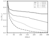Fig. 1.

Fraction of all stars that are present in their birth clusters at a given age, t, for clusters of initial mass M_ecl = 100 M_⊙ (dash-dotted line), M_ecl = 400 M_⊙ (dotted line), M_ecl = 1600 M_⊙ (dashed line), and M_ecl = 6400 M_⊙ (solid line).

The decrease of f_IC(M_ecl) with decreasing M_ecl is expected since lower-mass clusters are impacted more by gas expulsion (Baumgardt & Kroupa 2007) and have a shorter median two-body relaxation time-scale that leads to more rapid evaporation and cluster dissolution (Baumgardt & Makino 2003; Lamers et al. 2005).

4.2. Galaxy wide fraction of stars in clusters in a single starburst

We assume that embedded clusters are distributed according to the embedded cluster mass function (ECMF):

$\begin{matrix} ξ_{ecl} (M_{ecl}) \equiv \frac{d N_{ecl}}{d M_{ecl}} \propto M_{ecl}^{- β}, \end{matrix}$ $\begin{aligned} \xi _{\rm ecl} (M_{\rm ecl}) \equiv \frac{\mathrm{d} N_{\rm ecl}}{\mathrm{d} M_{\rm ecl}} \propto M_{\rm ecl}^{-\beta }, \end{aligned}$ (4)

where dN_ecl is the number of clusters in the mass bin (M_ecl, M_ecl + dM_ecl) and the index β is a parameter obtained from observations. Let a cluster of mass M_ecl have a property q(M_ecl), which is normalised by the total number of stars (q can be e.g. f_IC). Then, the same property for a coeval population of star clusters with mass range (M_ecl, min, M_ecl, max) is given by

$\begin{matrix} q_{pop} = \frac{\int_{M_{ecl, \min}}^{M_{ecl, \max}} ξ_{ecl} (M_{ecl}) q (M_{ecl}) M_{ecl} d M_{ecl}}{\int_{M_{ecl, \min}}^{M_{ecl, \max}} ξ_{ecl} (M_{ecl}) M_{ecl} d M_{ecl}} \cdot \end{matrix}$ $\begin{aligned} q_{\rm pop} = \frac{\int _{M_{\rm ecl, min}}^{M_{\rm ecl, max}} \xi _{\rm ecl} (M_{\rm ecl}) q(M_{\rm ecl}) M_{\rm ecl} \mathrm{d} M_{\rm ecl}}{\int _{M_{\rm ecl, min}}^{M_{\rm ecl, max}} \xi _{\rm ecl} (M_{\rm ecl}) M_{\rm ecl} \mathrm{d} M_{\rm ecl}}\cdot \end{aligned}$ (5)

We note that the integrals are mass weighted because the contribution of each mass bin dM_ecl is proportional to the total number of stars which formed within the mass bin, and thus in turn to the cluster mass M_ecl. In the following text, we refer to a quantity calculated by Eq. (5) as galaxy-wide. In the Galaxy and nearby galaxies, β ≈ 2 (van den Bergh & Lafontaine 1984; Whitmore et al. 1999; Larsen 2002; Lada & Lada 2003; Bik et al. 2003; de la Fuente Marcos & de la Fuente Marcos 2004; Gieles et al. 2006) and the cluster mass range covers approximately an interval of (30 M_⊙, 10⁴ M_⊙) (Johnson et al. 2017).

For an ECMF with these parameters, we obtain the time dependence of the galaxy wide fraction f_IC, pop of stars in clusters as shown in Fig. 2. We assume that all the clusters were formed in a single starburst, namely, that they are coeval. The plot is constructed for clusters orbiting at different galactocentric radii R_g and with different metallicities for R_g = 8 kpc. For all models, f_IC, pop drops significantly during the first 50 Myr of cluster evolution. This drop is dominated by the early gas expulsion, with the galactic tidal field being of secondary importance. At a given time, the value of f_IC, pop increases with increasing R_g as the tidal field of the galaxy becomes less important. In particular, at 200 Myr and for R_g = 4 kpc, 8 kpc and 12 kpc, f_IC, pop = 0.16, 0.25, and 0.32, respectively. The models with subsolar metallicities of Z = 0.002 and Z = 0.006 are shown by the dotted and dashed lines in Fig. 2, respectively. They indicate that f_IC, pop is practically independent of the metallicity of the clusters.

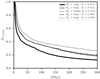Fig. 2.

Fraction of all stars located in their parent cluster for the galaxy-wide ECMF of Eq. (4) and for a single starburst. Clusters orbit the galaxy at R_g = 4 kpc, R_g = 8 kpc, and R_g = 12 kpc (different thickness of solid lines). These clusters have the Solar metallicity of Z = 0.014. Models of Z = 0.006 and Z = 0.002 for R_g = 8 kpc are shown by the dashed and dotted lines.

Figure 3 shows the time dependence of the galaxy-wide fraction f_IC, pop(m) of stars in clusters for stars of different masses, m, (or equivalently different spectral types). The figure demonstrates that the clusters mass segregate because the probability to find more massive stars (with the exception of O stars) in clusters at a given time is greater than the probability of finding lower-mass stars. The mass segregation is dynamical because these models are free of primordial mass segregation. At a given time, the fraction f_IC, pop(m) monotonically increases with stellar mass apart from the O stars because many O stars are ejected in close three- and multiple-body interactions producing runaway stars (e.g. Fujii & Portegies Zwart 2011; Tanikawa et al. 2012; Perets & Šubr 2012; Oh & Kroupa 2016). At the age of 200 Myr, only 19% of M stars are located in clusters, while 32% of late B stars are located in clusters.

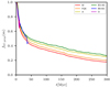Fig. 3.

Time dependence of the fraction of M (red line), F-K (orange), A (yellow), late B (green), early B (blue), and O (magenta) stars located in clusters for clusters with R_g = 8 kpc and Z = 0.014. The clusters are assumed to form with the ECMF of Eq. (4) with β = 2, M_ecl, min = 30 M_⊙, and M_ecl, max = 10⁴ M_⊙. At a given time, f_IC, pop(m) increases with stellar mass (apart from O stars), which is the result of dynamically induced mass segregation. The O stars are slightly depleted in clusters because of their dynamical ejections.

4.3. Fraction of stars in clusters in the context of the IGIMF in a single starburst

We explore the behaviour of f_IC, pop in the IGIMF framework, proposed by Kroupa & Weidner (2003) and further developed and refined by Weidner et al. (2013), Yan et al. (2017) and Jeřábková et al. (2018). According to IGIMF theory, the upper mass limit for star clusters, M_ecl, max, increases and β decreases with increasing SFR, so environments with larger SFR tend to form more massive clusters and these clusters are more abundant relative to the lower mass clusters. The SFR is taken from the whole galaxy. Thus, the IGIMF theory allows for the calculation of a galaxy-wide stellar population assuming all stars form in embedded star clusters. It successfully couples the molecular cloud-core scale to galaxy-wide properties such as the star formation rate.

We studied galaxies with SFRs of 0.01 M_⊙ yr⁻¹, 0.1 M_⊙ yr⁻¹, 1 M_⊙ yr⁻¹, 10 M_⊙ yr⁻¹, and 100 M_⊙ yr⁻¹. For each of these galaxies, we determined the mass of the most massive cluster according to Eq. (6) of (Weidner et al. 2004; see also Randriamanakoto et al. 2013), which is expressed as:

$\begin{matrix} M_{ecl, \max} = 8.5 \times 10^{4} M_{⊙} {(SFR / (M_{⊙} {yr}^{- 1}))}^{0.75} . \end{matrix}$ $\begin{aligned} M_{\rm ecl,max} = 8.5 \times 10^4\,M_{\odot } (\mathrm{SFR}/(M_{\odot }\,\mathrm{yr}^{-1}))^{0.75}. \end{aligned}$ (6)

Since galaxies with SFR ≳ 0.1 M_⊙ yr⁻¹ form clusters more massive than we can simulate easily (a 100 M_⊙ yr⁻¹ galaxy has M_ecl, max = 2.7 × 10⁶ M_⊙ according to Eq. (6), which is beyond the capability of even the most dedicated current software; Wang et al. 2015, 2020), we extrapolate²f_IC(M_ecl) from the five most massive clusters in our simulations towards higher mass at any time, t. The least massive clusters dissolve early, so we did not calculate extra models for M_ecl < 50 M_⊙, but extrapolate the values of f_IC(M_ecl) from the five least massive clusters in our simulations towards lower cluster masses.

The galaxy-wide fraction of stars in clusters as calculated by Eq. (5) is shown in Fig. 4. We assume that all the clusters were formed at the same time. In order to be consistent with the IGIMF framework, we set the ranges of the ECMF to be M_ecl, min = 5 M_⊙ and M_ecl, max according to Eq. (6), which is different from the cluster population considered in Sect. 4.2. Here, we take β and the SFR as independent variables to explore the admitted uncertainty in f_IC, pop; although in the strict sense of the IGIMF theory, β is a function of the SFR. According to the IGIMF theory, β ranges from 2.2 to 1.8 (Weidner et al. 2004; Jeřábková et al. 2018) in the considered range of SFR = 0.01 M_⊙ yr⁻¹ to SFR = 100 M_⊙ yr⁻¹. This is well within the extreme values for β of 1.5 and 2.4 considered in this work.

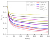Fig. 4.

Time dependence of the galaxy-wide f_IC, pop for galaxies with SFRs of 0.01 M_⊙ yr⁻¹, 0.1 M_⊙ yr⁻¹, 1 M_⊙ yr⁻¹, 10 M_⊙ yr⁻¹, and 100 M_⊙ yr⁻¹ (indicated by line colour) according to the IGIMF theory. The clusters have a metallicity of Z = 0.014 and orbit the galaxy at R_g = 8 kpc. The cluster mass range spans from 5 M_⊙ to M_ecl, max(SFR), which is given by Eq. (6). For each value of the SFR, we consider β = 1.5 (dashed lines), β = 2 (solid lines), and β = 2.4 (dotted lines).

For any β, at a given time, f_IC, pop increases with increasing SFR because of the increase of M_ecl, max. Particularly, for β = 2 at t = 200 Myr, f_IC, pop = 0.15, 0.35, and 0.48 for SFR of 0.01 M_⊙ yr⁻¹, 1 M_⊙ yr⁻¹, and 100 M_⊙ yr⁻¹, respectively. The ECMF of a shallower slope of β = 1.5 (dashed lines in Fig. 4) produces more massive clusters relative to the lower mass ones, these clusters dissolve at a slower rate, which results in an increase of f_IC, pop at a given time. In contrast, ECMFs of a steeper slope (β = 2.4; dotted lines) form more low mass clusters, which are easily disrupted, which results in a lower value of f_IC, pop. The likely observed fraction of stars in clusters within a galaxy of SFR = 1 M_⊙ yr⁻¹ (Milky Way-like SFR) in IGIMF theory (but with β taken as a free parameter) is shown in the right panel of Fig. A.1.

4.4. Fraction of stars in clusters for a galaxy with a constant rate of star formation

In the previous two sections, Sects. 4.2 and 4.3, we studied f_IC, pop for star clusters that all formed in a single starburst. Here, we consider the opposite scenario, that is, where star formation proceeds continuously, with the SFR constant over time. The particular value of the SFR is not important as long as it allows us to fully sample the upper limit of the ECMF because of the normalisation to the total number of stars formed. The results are relevant to stars younger than 300 Myr only because of the duration of our simulations. Such a star formation history produces a time-independent fraction ${\bar{f}}_{IC, pop} (t < 300 Myr)$ $\overline{f}_{\mathrm{IC,pop}} (t < 300\,\mathrm{Myr})$ of stars in clusters (listed in Table 1).

Table 1.

The fraction of stars in clusters ${\bar{f}}_{IC, pop} (t < 300 Myr)$ $\overline{f}_{\mathrm{IC,pop}} (t < 300\,\mathrm{Myr})$ for a time-independent SFR for stars younger than 300 Myr.

The first three lines of the table feature star clusters with (M_ecl, min, M_ecl, max) = (30 M_⊙, 10⁴ M_⊙) and β = 2. In these models, we use the same cluster mass range at all the galactocentric radii R_g to study the influence of the tidal field strength. For these clusters, ${\bar{f}}_{IC, pop} (t < 300 Myr)$ $\overline{f}_{\mathrm{IC,pop}} (t < 300\,\mathrm{Myr})$ increases with increasing R_g from 0.26 for R_g = 4 kpc to 0.41 for R_g = 12 kpc.

There is evidence that the mass of the most massive cluster decreases with the local gas column density (Pflamm-Altenburg & Kroupa 2008). In disc galaxies, the dependence can be approximated as ∝exp(−3R_g/2R_d), where R_d is the disc scale-length. Taking this dependence into account (with R_d = 4 kpc), we obtain ${\bar{f}}_{IC, pop} (t < 300 Myr)$ $\overline{f}_{\mathrm{IC,pop}} (t < 300\,\mathrm{Myr})$ decreasing with R_g from 0.36 for R_g = 4 kpc to 0.29 for R_g = 12 kpc (second group of models in Table 1). Thus, the decreasing M_ecl, max with R_g shows the opposite trend from the decreasing tidal field strength (as discussed in the previous paragraph) and, in addition, it has more impact on ${\bar{f}}_{IC, pop}$ $\overline{f}_{\mathrm{IC,pop}}$ than the tidal field.

The third group of records in Table 1 lists the time-averaged fractions of stars in clusters for stars in six different mass bins for clusters with R_g = 8 kpc and M_ecl, max = 10⁴ M_⊙. The value of ${\bar{f}}_{IC, pop} (m, t < 300 Myr)$ $\overline{f}_{\mathrm{IC,pop}}(m, t < 300\,\mathrm{Myr})$ increases monotonically with stellar mass from 0.32 for M stars to 0.41 for late B (B3-A0) stars. Stars that are even more massive have substantially higher ${\bar{f}}_{IC, pop} (m, t < 300 Myr,$ $\overline{f}_{\mathrm{IC,pop}}(m, t < 300\,\mathrm{Myr},$ reaching 0.83 for O and early B stars) not only as the result of dynamical mass segregation, but also because they are present only in the youngest clusters, which have had not enough time to dissolve.

The last 15 lines of Table 1 represent the results with the cluster mass limits (M_ecl, min, M_ecl, max) set according to IGIMF theory (Sect. 4.3). The table shows the same trend as we encountered in Sect. 4.3: ${\bar{f}}_{IC, pop} (t < 300 Myr)$ $\overline{f}_{\mathrm{IC,pop}} (t < 300\,\mathrm{Myr})$ increases with increasing SFR and decreasing β. For models with a top-heavy ECMF (β = 1.5), ${\bar{f}}_{IC, pop} (t < 300 Myr)$ $\overline{f}_{\mathrm{IC,pop}} (t < 300\,\mathrm{Myr})$ strongly depends on the SFR: ${\bar{f}}_{IC, pop} (t < 300 Myr)$ $\overline{f}_{\mathrm{IC,pop}} (t < 300\,\mathrm{Myr})$ increases by more than a factor of 2 from ${\bar{f}}_{IC, pop} (t < 300 Myr) = 0.39$ $\overline{f}_{\mathrm{IC,pop}} (t < 300\,\mathrm{Myr}) = 0.39$ for SFR = 0.01 M_⊙ yr⁻¹ to ${\bar{f}}_{IC, pop} (t < 300 Myr) = 0.84$ $\overline{f}_{\mathrm{IC,pop}} (t < 300\,\mathrm{Myr}) = 0.84$ for SFR = 100 M_⊙ yr⁻¹. On the other hand, models with a top-light ECMF (β = 2.4) have ${\bar{f}}_{IC, pop} (t < 300 Myr)$ $\overline{f}_{\mathrm{IC,pop}} (t < 300\,\mathrm{Myr})$ almost independent of SFR because such a steep β ensures that there are very few massive star clusters, which would contribute to a higher ${\bar{f}}_{IC, pop} (t < 300 Myr)$ $\overline{f}_{\mathrm{IC,pop}} (t < 300\,\mathrm{Myr})$ .

The model of β = 2 and SFR = 1 M_⊙ yr⁻¹ is close to the Galaxy in the IGIMF framework, which includes the cluster population of the whole Galaxy. This model provides ${\bar{f}}_{IC, pop} (t < 300 Myr) = 0.42$ $\overline{f}_{\mathrm{IC,pop}} (t < 300\,\mathrm{Myr}) = 0.42$ . Since the mass of the most massive cluster decreases with the local gas column density (Pflamm-Altenburg & Kroupa 2008), the majority of the most massive star clusters in the Galaxy are located near the Galactic centre or tips of the bar (Portegies Zwart et al. 2010), and the environment in the vicinity of the Sun hosts clusters with masses only up to M_ecl, max ≈ 4000 M_⊙. This cluster mass limit provides ${\bar{f}}_{IC, pop} (t < 300 Myr) = 0.26$ $\overline{f}_{\mathrm{IC,pop}} (t < 300\,\mathrm{Myr}) = 0.26$ , which is by ≈40% lower than what we obtain for the Galaxy as a whole.

4.5. Comparison to observations and to the current theoretical model

The observations of Chandar et al. (2017) present results for eight galaxies. We focus particularly on Small and Large Magellanic Clouds, because they differ most from the Γ − Σ_SFR model (the two data points with the lowest Σ_SFR in Fig. 5) at their youngest age. These data points utilise the cluster catalogue of Hunter et al. (2003), which is based on visual inspection of cluster candidates from previous catalogues. Hunter et al. (2003) take a candidate object as a cluster if it is distinguishable from the background galaxy within a circle of radius 23″ (5.5 pc at the distance of 50 kpc) and resolved at least to several stars. This makes our simulations difficult to be directly compared with observations because we cannot automatically identify star clusters in our simulations based on exactly defined criteria.

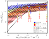Fig. 5.

Likely detected fraction of stars in clusters of age t < 10 Myr (blue area and blue lines), 10 Myr < t < 100 Myr (yellow area and yellow lines), and 100 Myr < t < 300 Myr (red area and red lines) as a function of Σ_SFR. Apart from indicating age by colour, age is also shown by a hatch style. The coloured area is bordered by two extreme models: the lower one has β = 2.2 and r_search = 2 pc, the upper one has β = 1.8 and r_search = 5 pc. The models for β = 2.0 and r_search = 2 pc and 5 pc are shown by the dashed lines. The plot shows how ${\bar{f}}_{IC, pop}^{obs}$ $\overline{f}^{\mathrm{obs}}_{\mathrm{IC,pop}}$ increases with the Σ_SFR, and how it decreases with the cluster age. The observational data from Chandar et al. (2017), which are aimed consistently at galaxies both with low SFR and high SFR, are shown by empty squares with their errorbars. Our results are obtained at almost the same time intervals as the observational data (indicated by the colours). The semi-analytic estimate provided by the Γ − Σ_SFR model is shown by the black solid line. We note its disagreement with the observational data for the clusters of any age interval.

To provide an order of magnitude estimate, we place a circle of radius r_search at the cluster density centre, and count the number of stars located within the projected circle. If at least ten stars of spectral type A and earlier are found, we consider the cluster to be detected, and we count the stars within radius r_search as the cluster population, while the rest of the stars count to the field population. Otherwise, we do not consider the cluster as having been detected and, thus, we count all stars in it as the field population. To estimate the sensitivity of this method, we use two radii: 2 pc and 5 pc, the latter one being close to the radius ≈5.5 pc adopted by Hunter et al. (2003).

Figure 5 compares the fraction of stars detected by the method described above in our simulations (hatched areas and dashed lines) with the observational data from Chandar et al. (2017), shown as empty squares with error bars. The SFR is related to the Σ_SFR on the assumption that each galaxy has a star formation area of 100 kpc²; this order of magnitude estimate is compatible with the galaxies studied by Chandar et al. (2017, cf. their Table 1). We evaluate ${\bar{f}}_{IC, pop}^{obs}$ $\overline{f}^{\mathrm{obs}}_{\mathrm{IC,pop}}$ at the same time intervals as the observational data except the oldest age interval, which we take from 100 Myr to 300 Myr, while the observations take it from 100 Myr to 400 Myr. The hatched areas cover the range of β ∈ (1.8, 2.2) and r_search between 2 and 5 pc, while the dashed lines show the value of ${\bar{f}}_{IC, pop}^{obs}$ $\overline{f}^{\mathrm{obs}}_{\mathrm{IC,pop}}$ for β = 2 and r_search = 2 pc and 5 pc. The youngest clusters (blue symbols and lines; age < 10 Myr) have ${\bar{f}}_{IC, pop}^{obs}$ $\overline{f}^{\mathrm{obs}}_{\mathrm{IC,pop}}$ comparable to observations, while older clusters have ${\bar{f}}_{IC, pop}^{obs}$ $\overline{f}^{\mathrm{obs}}_{\mathrm{IC,pop}}$ higher than in observations. Thus, the rough approximation to ‘synthetic observations’ is in agreement with the original hypothesis that all stars originate in gravitationally bound embedded clusters. Gas expulsion not only unbinds many stars from the clusters, but also decreases their density so that many of the youngest clusters cannot be detected, an idea originally proposed by Lüghausen et al. (2012). The overestimation of ${\bar{f}}_{IC, pop}$ $\overline{f}_{\mathrm{IC,pop}}$ in older clusters can be caused by neglecting the interaction of clusters with molecular clouds in our models, which probably plays an important role in cluster dissolution (Terlevich 1987; Lamers & Gieles 2006; Chandar et al. 2010; Jerabkova et al. 2021).

Only the youngest objects can be compared with the Γ − Σ_SFR theory because the theory does not consider any process that releases stars after the clusters emerge from their natal clouds, which occurs at the age of several Myr. This constraints the comparison to the youngest objects (10 Myr; blue lines and squares in Fig. 5), which are the least impacted by dynamical evolution. Thus, $Γ \approx {\bar{f}}_{IC, pop} (t < 10 Myr)$ $\Gamma \approx \overline{f}_{\mathrm{IC,pop}} (t < 10\,\mathrm{Myr})$ . For low SFRs, Γ-1 models predict substantially larger values of ${\bar{f}}_{IC, pop}^{obs} (t < 10 Myr)$ $\overline{f}^{\mathrm{obs}}_{\mathrm{IC,pop}}(t < 10\,\mathrm{Myr})$ in contrast to the Γ − Σ_SFR model: for Σ_SFR = 10⁻⁴ M_⊙ yr⁻¹ kpc⁻², the admitted values of ${\bar{f}}_{IC, pop}^{obs} (t < 10 Myr)$ $\overline{f}^{\mathrm{obs}}_{\mathrm{IC,pop}}(t < 10\,\mathrm{Myr})$ in Γ-1 models range from 0.07 to 0.45, while the Γ − Σ_SFR model predicts Γ = 0.0015³. For high SFRs, the Γ-1 model predicts lower ${\bar{f}}_{IC, pop}^{obs} (t < 10 Myr)$ $\overline{f}^{\mathrm{obs}}_{\mathrm{IC,pop}}(t < 10\,\mathrm{Myr})$ in contrast to the Γ − Σ_SFR model.

In the Γ − Σ_SFR model as well as in the Γ-1 model, Γ increases with Σ_SFR. However, the reason for this behaviour is very different in this case. In the Γ − Σ_SFR model, it is the combined effect of the increasing SFE(x) and γ(x) with x, where high values of x are reached as the ISM probability distribution function widens with increasing ρ_ISM (via the ISM Mach number). In contrast, in the Γ-1 model, the increase is due to the expansion and partial dissolution of clusters as the result of gas expulsion, which has a lesser impact on more massive clusters, which according to the IGIMF theory form only in galaxies with a sufficiently high Σ_SFR. Another difference is the much weaker dependence of Γ on Σ_SFR, which was noted by Chandar et al. (2017) and is reproduced in the Γ-1 model.

5. Discussion

5.1. Influence of the initial conditions of star clusters

To calculate the present models, we adopted a set of specific initial conditions, which are described in Sect. 3.1.1. However, both observational and theoretical evidence indicates that the initial conditions for star cluster formation are not fully understood. For example, the value of the SFE, initial cluster radii, the time-scale of gas expulsion, and the degree of primordial mass segregation are subject to ongoing research (e.g. Er et al. 2013; Kuhn et al. 2014; Banerjee & Kroupa 2015; Megeath et al. 2016; Spera & Capuzzo-Dolcetta 2017; Domínguez et al. 2017; Pfalzner 2019; Kuhn et al. 2019; Dib & Henning 2019; Pang et al. 2020). Some of the cluster initial conditions are interrelated: for example, embedded star clusters cannot form with sub-parsec scales and SFE close to 100% because they would not be able to expand to their observed sizes (Banerjee & Kroupa 2017).

5.1.1. Initial cluster radius and the SFE

To study the possible influence of the initial cluster radius and the SFE, we perform additional models with clusters of slightly larger radii (by at most a factor of 3; ‘A’ models) and clusters of a slightly lower SFE of 0.25 (‘F’ models; see Sect. 3.1.2 for the model descriptions). The time dependence of f_IC(M_ecl) for clusters of four different masses is shown in Fig. 6. In comparison to the standard models (“S” models), both ‘A’ and ‘F’ models release stars to the field earlier, and have a faster cluster dissolution. Also, the most massive clusters in our sample (6400 M_⊙) have lost most of their stars already by 30 Myr in the ‘A’ and ‘F’ models, while the clusters are relatively unaffected in the standard models even at 300 Myr.

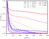Fig. 6.

Fraction of stars located in clusters of an initial mass M_ecl for ‘A’ models (blue lines) and ‘F’ models (magenta lines). For comparison, standard models are shown by red lines. The ‘A’ and ‘F’ models result in substantially lower fraction of stars in clusters of all considered masses at t ≳ 20 Myr.

For a Milky Way-like galaxy with a constant SFR and star formation parameters β = 2 and SFR = 1 M_⊙ yr⁻¹, ‘A’ and ‘F’ models have only ${\bar{f}}_{IC, pop} (t < 300 Myr) = 0.11$ $\overline{f}_{\mathrm{IC,pop}} (t < 300\,\mathrm{Myr}) = 0.11$ and 0.06, respectively, while it is 0.42 in standard models. The difference in f_IC, pop between the models is small in the youngest clusters, but it becomes more pronounced over time. Model ‘A’ has the interesting property of f_IC, pop(M_ecl) being almost independent of the cluster mass by ≈150 Myr for the cluster mass range spanning more than one order of magnitude from ≈400 M_⊙ to ≈6400 M_⊙. This property is not seen in models ‘F’ and ‘S’, which have a smaller cluster radii. This behaviour is in line with the observations indicating that the dissolution rate of star clusters is independent of their initial mass (e.g. Lada & Lada 2003; Fall et al. 2005; Whitmore et al. 2007), but such an explanation is only hypothetical for now given the model uncertainties and the uncertain role of molecular clouds in cluster dissolution.

The physical reason for the faster release of stars from clusters in the ‘A’ models is due to gas expulsion occurring more impulsively, namely, the ratio between the gas expulsion time-scale and the cluster crossing time, τ_M/t_cross, being smaller. Since $τ_{M} / t_{cross} \propto \sqrt{M_{ecl} / a_{ecl}}$ $\tau_{\mathrm{M}}/t_{\mathrm{cross}} \propto \sqrt{M_{\mathrm{ecl}}/a_{\mathrm{ecl}}}$ and $a_{ecl} \propto M_{ecl}^{1 / 3}$ $a_{\mathrm{ecl}} \propto M_{\mathrm{ecl}}^{1/3}$ , the difference between the ‘A’ and ‘S’ models increases with increasing cluster mass. The impact of gas expulsion increases strongly when τ_M/t_cross becomes smaller than unity (Baumgardt & Kroupa 2007), which is the case of all clusters in the ‘A’ models. The most massive clusters (M_ecl = 6400 M_⊙) have τ_M/t_cross = 1 for ‘S’ models, while it is 0.63 for ‘A’ models. Because of the monotonic increase of the ratio τ_M/t_cross with M_ecl (as $M_{ecl}^{1 / 3}$ $M_{\mathrm{ecl}}^{1/3}$ for ‘A’ models), clusters with M_ecl < 6400 M_⊙ have τ_M/t_cross < 0.63, resulting in their rapid dissolution. The reason for the faster release of stars from clusters in ‘F’ models is due to their lower SFE (Baumgardt & Kroupa 2007).

Figure 7 shows the fraction of stars which is likely to be observed in clusters for the ‘S’, ‘A’, and ‘F’ models assuming IGIMF theory and β = 2. For the youngest clusters (t ≲ 10 Myr; blue lines), the difference between the models varies less than by a factor of three; it decreases from ${\bar{f}}_{IC, pop}^{obs} (t < 10 Myr) \approx 0.35$ $\overline{f}_{\mathrm{IC,pop}}^{\mathrm{obs}} (t < 10\,\mathrm{Myr}) \approx 0.35$ for S models to ${\bar{f}}_{IC, pop}^{obs} (t < 10 Myr) \approx 0.13$ $\overline{f}_{\mathrm{IC,pop}}^{\mathrm{obs}} (t < 10\,\mathrm{Myr}) \approx 0.13$ for ‘F’ models (for Milky Way-like Σ_SFR of ≈1 M_⊙ yr⁻¹). Similar to the ‘S’ models, both ‘A’ and ‘F’ models reasonably agree with the observations, and they show a much weaker dependence on Σ_SFR than predicted by the Γ − Σ_SFR theory.

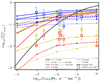Fig. 7.

Fraction of stars which is likely to be observed in clusters of age t < 10 Myr (blue lines), 10 Myr < t < 100 Myr (yellow lines), and 100 Myr < t < 300 Myr (red lines) as a function of Σ_SFR. The plot shows results for the ‘S’, ‘A’, and ‘F’ models for the ECMF of slope β = 2 by solid, dashed, and dotted lines, respectively. The lines are shown for r_search = 2 pc (smaller dots) and r_search = 5 pc (larger dots) for each model. The prediction of the Γ − Σ_SFR model and the observational data from Chandar et al. (2017) are shown by the black line and by squares, respectively.

For older clusters (age ≳ 10 Myr; yellow and red lines in Fig. 7), the ‘A’ and ‘F’ models result in significantly lower observed fractions of stars in clusters than in the standard model. This brings ‘A’ and ‘F’ models closer to the observations of Chandar et al. (2017) also at later times; the modelled values of ${\bar{f}}_{IC, pop}^{obs} (10 Myr < t < 100 Myr)$ $\overline{f}_{\mathrm{IC,pop}}^{\mathrm{obs}} (10\,\mathrm{Myr} < t < 100\,\mathrm{Myr})$ and ${\bar{f}}_{IC, pop}^{obs} (t < 300 Myr)$ $\overline{f}_{\mathrm{IC,pop}}^{\mathrm{obs}} (t < 300\,\mathrm{Myr})$ are even lower than the observations. The ‘F’ models have a too low a fraction of stars in clusters. This indicates that the observational data could be well reproduced also for clusters older than 10 Myr and as old as at least 300 Myr by either steepening the relationship between the cluster mass and its radius, or by lowering the SFE (although the latter possibility requires the SFE to be somewhere between 0.25 and 0.33) without considering any additional cluster dissolving mechanism such as interactions with molecular clouds. This is a remarkable property that characterises ‘A’ and ‘F’ models because standard models necessitate an additional cluster dissolving mechanism to explain the observations for t ≳ 10 Myr (Sect. 4.5). Given the large sensitivity of the fraction of stars in clusters on the SFE and possibly τ_M, it is probable that the observations for clusters up to the age of at least 300 Myr can be explained by more combinations of the cluster parameters (a_ecl, SFE and τ_M) than those considered in this work.

The impact of gas expulsion on a cluster is a strong function of the ratio τ_M/t_cross (Lada et al. 1984; Baumgardt & Kroupa 2007). For all the clusters studied in this work, gas expulsion is impulsive (τ_M/t_cross ≲ 1). Assuming τ_M = 10 km s⁻¹ independent of M_ecl, gas expulsion becomes adiabatic (τ_M/t_cross ≫ 1) if M_ecl ≫ 10⁴ M_⊙. Adiabatic gas expulsion unbinds a substantially lower fraction of stars than impulsive gas expulsion (e.g. Lada et al. 1984). Since we extrapolate results from clusters with impulsive gas expulsion towards the more massive ones with adiabatic gas expulsion, f_IC(M_ecl) is underestimated for M_ecl ≳ 10⁴ M_⊙. We estimate that this effect is of secondary importance (at least for the clusters in the youngest age bin) because f_IC(M_ecl = 6400 M_⊙)≳0.8 (Fig. 1). Even if f_IC(M_ecl) were 1 for M_ecl ≳ 10⁴ M_⊙, ${\bar{f}}_{IC, pop} (t < 10 Myr)$ $\overline{f}_{\mathrm{IC,pop}} (t < 10\,\mathrm{Myr})$ cannot differ by more than a factor of 1/0.8 = 1.25 from the present models.

The models with SFE = 0.25 present a lower estimate on the SFE because they underestimate the fractions of stars in clusters after 10 Myr (Fig. 7). In the other extreme, we consider the expected fraction of stars in clusters in the absence of gas expulsion (i.e. SFE = 1). In this case, the clusters would be unaffected, so they would resemble their state at t = 0, at which time ${\bar{f}}_{IC, pop}^{obs} (0) = 0.61$ $\overline{f}_{\mathrm{IC,pop}}^{\mathrm{obs}} (0) = 0.61$ for a Milky Way-like galaxy (Σ_g = 1 M_⊙ pc⁻² and β = 2). The present simulations predict ${\bar{f}}_{IC, pop}^{obs} (t < 10 Myr) \approx 0.35$ $\overline{f}_{\mathrm{IC,pop}}^{\mathrm{obs}} (t < 10\,\mathrm{Myr}) \approx 0.35$ . Thus, the uncertainty in gas expulsion parameters can increase the value of ${\bar{f}}_{IC, pop}^{obs} (t < 10 Myr)$ $\overline{f}_{\mathrm{IC,pop}}^{\mathrm{obs}} (t < 10\,\mathrm{Myr})$ by at most a factor of 1.8.

5.1.2. Primordial mass segregation

To study the possible influence of the initial conditions on the fraction of stars to be found in clusters, we perform additional models with a high degree of primordial mass segregation (models ‘M’), which are detailed in Sect. 3.1.2. These models present likely the extreme cases of stellar concentrations within the clusters, having a very compact core of massive stars, while the standard (‘S’ models) are of a more uniform density. Figure 8 compares the time dependence of f_IC(m) for a cluster of mass 400 M_⊙ between the ‘S’ and ‘M’ models.

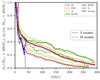Fig. 8.

Time dependence of f_IC(m) for clusters of mass 400 M_⊙ starting with initial conditions for models ‘S’ (solid lines) and ‘M’ (dashed lines). The values of f_IC(m) for different stellar spectral types is shown by line colours. The fraction of all stars in clusters f_IC(M_ecl = 400 M_⊙) is shown by the black lines. The clusters orbit the galaxy at R_g = 8 kpc and they have metallicity of Z = 0.014.

Generally, all the models have f_IC(m) increasing with m at a given time, which reflects mass segregation, which is established dynamically in the ‘S’ models. The primordially mass-segregated ‘M’ clusters lose stars more quickly and dissolve earlier than their non-mass segregated ‘S’ counterparts. Assuming that we observe clusters of mass 400 M_⊙, which formed in a galaxy with a constant SFR over an extended time interval (longer than 300 Myr), the fraction of stars found in these clusters is ${\bar{f}}_{IC} (t < 300 Myr) = 0.26$ $\overline{f}_{\mathrm{IC}}(t < 300\,\mathrm{Myr}) = 0.26$ for the ‘S’ models and ${\bar{f}}_{IC} (t < 300 Myr) = 0.17$ $\overline{f}_{\mathrm{IC}}(t < 300\,\mathrm{Myr}) = 0.17$ for the ‘M’ models. These values are for all stars in gravitationally bound objects, many of which are comprised from only tens of stars, and are not likely to be observed. The same estimate of the fraction of observable stars in clusters (as detailed in Sect. 4.5) yields, for ‘S’ models: ${\bar{f}}_{IC}^{obs} (t < 10 Myr) = 0.34$ $\overline{f}_{\mathrm{IC}}^{\mathrm{obs}} (t < 10\,\mathrm{Myr}) = 0.34$ and ${\bar{f}}_{IC}^{obs} (t < 10 Myr) = 0.49$ $\overline{f}_{\mathrm{IC}}^{\mathrm{obs}} (t < 10\,\mathrm{Myr}) = 0.49$ for r_search = 2 pc and 5 pc, respectively. The ‘M’ models have slightly lower fractions of the youngest stars in clusters, ${\bar{f}}_{IC}^{obs} (t < 10 Myr) = 0.31$ $\overline{f}_{\mathrm{IC}}^{\mathrm{obs}} (t < 10\,\mathrm{Myr}) = 0.31$ and ${\bar{f}}_{IC}^{obs} (t < 10 Myr) = 0.48$ $\overline{f}_{\mathrm{IC}}^{\mathrm{obs}} (t < 10\,\mathrm{Myr}) = 0.48$ for r_search = 2 pc and 5 pc, respectively. Thus, primordial mass segregation decreases ${\bar{f}}_{IC}$ $\overline{f}_{\mathrm{IC}}$ in a population of clusters, but its observed manifestation in the youngest age group is modest.

We expect that the difference of ${\bar{f}}_{IC}^{obs} (t < 10 Myr)$ $\overline{f}_{\mathrm{IC}}^{\mathrm{obs}} (t < 10\,\mathrm{Myr})$ between the ‘M’ and ‘S’ models decreases for clusters more massive than 400 M_⊙ because more massive clusters tend to retain more of their stars, and the difference increases for clusters of mass below 400 M_⊙ for the opposite reason⁴. In total, we expect that for a population of primordially mass segregated clusters with β = 2, ${\bar{f}}_{IC}^{obs} (t < 10 Myr)$ $\overline{f}_{\mathrm{IC}}^{\mathrm{obs}} (t < 10\,\mathrm{Myr})$ is slightly lower (approximately up to a factor of 1.2) than for the non-mass segregated clusters.

5.2. Influence of the form of the ECMF

The admitted variation of the slope β, which ranges from 1.8 to 2.2 in most galaxies (e.g. Whitmore et al. 1999; Lada & Lada 2003; Chandar et al. 2010), results in the ‘observed’ variation of the fraction of stars in the youngest clusters to vary in the range of ${\bar{f}}_{IC}^{obs} (t < 10 Myr) = 0.18$ $\overline{f}_{\mathrm{IC}}^{\mathrm{obs}} (t < 10\,\mathrm{Myr}) = 0.18$ to 0.55 (for a Milky Way-like galaxy with Σ_g = 1 M_⊙ pc⁻²). It differs by a factor of 2 from the standard value for β = 2. This uncertainty is of a comparable magnitude as the uncertainty in the initial cluster conditions.

Another important parameter of the ECMF is the cluster lower mass limit M_ecl, min. Chandar et al. (2017) use M_ecl, min = 100 M_⊙, while the formation of clusters of mass significantly lower than that is known (e.g. Kroupa & Bouvier 2003; Kirk & Myers 2011; Joncour et al. 2018; Plunkett et al. 2018). Decreasing the lower mass cluster limit results in a higher value of Γ. For example, for the LMC, Chandar et al. (2017) obtained Γ = 0.27, while it would be Γ = 0.41 for M_ecl, min = 5 M_⊙. Taking into account a lower mass limit, M_ecl, min, would bring their observations towards a better agreement with our models.

5.3. Comparison to observations

An important step in determining the value of Γ is to identify all clusters above a given mass limit M_ecl, lim (typically M_ecl, lim > M_ecl, min; Goddard et al. 2010; Chandar et al. 2017). Then, the total cluster population is obtained by extrapolating the number of clusters towards M_ecl lower than M_lim assuming an ECMF slope β. Even clusters with mass above M_ecl, lim suffer from incompleteness mainly due to extinction, where some clusters are obscured by molecular clouds and crowding in the most active star forming regions. These observational limitations tend to underestimate Γ. Taking this aspect into account could improve the agreement between our model and observations in galaxies with higher SFRs, as seen in Fig. 5.

6. Conclusions

We investigated whether the majority of stars form in gravitationally bound or unbound systems using N-body simulations. As a starting hypothesis, we assumed that Γ = 1, that is, that all stars form in gravitationally bound embedded clusters. This hypothesis is consistent with and motivated by observational data of young star forming regions. The clusters experience a gravitational potential drop as the result of early gas expulsion, which impacts low-mass clusters more strongly than higher-mass clusters. Additional stars escape their initial host clusters due to ejection, evaporation, and the tidal field of the host galaxy.

The time evolution of the fraction of stars in clusters for all clusters originating in a single coeval star burst is shown in Fig. 4. For example, in a Milky Way-like galaxy (SFR ≈ 1 M_⊙ yr⁻¹) with the ECMF slope β = 2, our simulations predict that 35% of stars remain gravitationally bound to their initial host clusters at the age of 200 Myr. More massive stars are more likely to be present in clusters (83% of O-type stars) than lower-mass stars (32% of M-type stars younger than 300 Myr; Table 1).

The galactic tidal field disrupts clusters more easily at smaller galactocentric distances R_g; assuming the same upper cluster mass limit throughout the galaxy, the fraction of stars in clusters increases by a factor of 1.6 between R_g = 4 kpc and R_g = 12 kpc for β = 2 (Table 1). However, in a more realistic scenario where the upper cluster mass limit decreases with increasing R_g, the fraction of stars in clusters decreases by a factor of 1.2 from R_g = 4 kpc to R_g = 12 kpc – thus more than compensating for the impact of the tidal field. The influence of cluster metallicity is negligible. If clusters form as primordially mass-segregated, the fraction of stars in clusters is slightly lower, but likely not more than by a factor of 1.2.

We compared our simulations to the observations. This comparison is deemed approximate because of the systematic differences in detecting star clusters and their member stars observationally versus within our simulations. For the youngest stars (t < 10 Myr), our models are in agreement with most of the observational data of Chandar et al. (2017) (Fig. 5). Thus, the observations are in agreement with the hypothesis that all stars form in gravitationally bound embedded clusters. We further find a rather weak dependence of the fraction ${\bar{f}}_{IC, pop}^{obs} (t < 10 Myr)$ $\overline{f}_{\mathrm{IC, pop}}^{\mathrm{obs}}(t < 10\,\mathrm{Myr})$ of the observed youngest stars in clusters on Σ_SFR, which is contrast to the strong dependence posited by the Γ − Σ_SFR model (Kruijssen 2012). These results show only weak sensitivity on the particular choice of parameters for our model such as the initial cluster radius or the SFE. The physical reason for the dependence of ${\bar{f}}_{IC, pop}^{obs}$ $\overline{f}_{\mathrm{IC, pop}}^{\mathrm{obs}}$ on Σ_SFR is different from the dependence in the Γ − Σ_SFR model: in our model, it is due to the lesser impact of gas expulsion on more massive clusters, which takes place predominantly in galaxies with higher Σ_SFR; whereas it is due to star formation at higher gas densities, higher SFEs, and a higher fraction of stars forming in bound clusters in the Γ − Σ_SFR model.

At later times (ages between 10 to 100 Myr and 100 to 300 Myr; Fig. 5), our standard models have too large values of ${\bar{f}}_{IC, pop}^{obs}$ $\overline{f}_{\mathrm{IC, pop}}^{\mathrm{obs}}$ as compared to observations. A similar result was previously found by Lamers et al. (2005), who did not include early gas expulsion. Thus, early gas expulsion does not reconcile this discrepancy, and other mechanisms (e.g. encounters with giant molecular clouds) are needed to reduce the number of clusters and bring them closer to the observed values. A case in point are the nearby Hyades star cluster, which may be in the process of being disrupted (Jerabkova et al. 2021).

We propose an alternative explanation to this picture. The difference between N-body models and observations could be reconciled by adjusting some parameters of our models (Sect. 5.1.1), the most attractive of which is the SFE and the relationship between the cluster half-mass radius and cluster mass. In this case, the gas expulsion, cluster dynamics, and galactic potential alone bring the results closer to the observations (at least for clusters younger than 300 Myr) without the necessity of employing additional cluster dissolution mechanisms.

We contrast the dynamical paradigm where all stars form in embedded clusters with the theoretical Γ − Σ_SFR framework that derives the functional form of Γ(Σ_SFR) by combining the observed and modelled properties of the ISM and star-forming regions. We identify several questionable points in the Γ − Σ_SFR theory, particularly the substitution of several equations into one another, some of which are non-linear or contain uncertain or poorly constrained terms. Additionally, the Γ − Σ_SFR framework neglects early stellar feedback, Larson’s relations, the time-dependent star formation rate during cluster formation, stellar dynamics, and the density threshold for star formation. Using a toy model, we show (in Sect. 2.2) that even small changes to the equations (that are consistent with observations) assumed by the Γ − Σ_SFR model result in very different functional forms of Γ as a function of Σ_SFR. This leads us to challenge the key prediction of the Γ − Σ_SFR model: that most stars form as non-gravitationally bound with regard to embedded star clusters in Milky Way-like galaxies. Instead, we suggest that cluster dynamics, early gas expulsion, and the influence of realistic galactic environments (potential and giant molecular clouds) provide an explanation for the fraction of stars observed in star clusters under the hypothesis that all stars originate from gravitationally bound systems.

¹

The sensitivity to the choice of the particular functional forms was mentioned by Kruijssen (2012, their Appendix D), although its influence on results was not investigated or discussed in detail.

²

From the requirement that the extrapolation function tends to 1 for M_ecl → ∞ and to 0 for M_ecl → 0, we adopt the extrapolation function in the form of

$\begin{matrix} y ({log}_{10} (M_{ecl})) = \frac{1}{π} {\frac{π}{2} + arctan (a ({log}_{10} (M_{ecl})) - b)}, \end{matrix}$ $\begin{aligned} y(\log _{10}(M_{\rm ecl})) = \frac{1}{\pi } \left\{ \frac{\pi }{2} + \arctan (a({\log }_{10}(M_{\rm ecl})) - b)\right\} , \end{aligned}$ (7)

where a and b are the unknowns.

³

We note that we compare the ‘observed’ fraction of stars in clusters in the Γ-1 model (i.e. ${\bar{f}}_{IC, pop}^{obs} (t < 10 Myr)$ $\overline{f}^{\mathrm{obs}}_{\mathrm{IC,pop}}(t < 10\,\mathrm{Myr})$ ) with the physical fraction (i.e. Γ) of the Γ − Σ_SFR model. However, the observed fraction of stars in clusters is always lower than the physical fraction (i.e., ${\bar{f}}_{IC, pop}^{obs} (t < 10 Myr) < {\bar{f}}_{IC, pop} (t < 10 Myr)$ $\overline{f}^{\mathrm{obs}}_{\mathrm{IC,pop}}(t < 10\,\mathrm{Myr}) < \overline{f}_{\mathrm{IC,pop}}(t < 10\,\mathrm{Myr})$ ) because of incompleteness, which makes the difference with the Γ − Σ_SFR model even more pronounced.

⁴

We chose for the cluster mass to be 400 M_⊙ because it lies approximately in between the interval (log₁₀(M_ecl, min), log₁₀(M_ecl, max)), i.e. the total number of stars contained in clusters forming within mass interval (M_ecl, min, 400 M_⊙) and (400 M_⊙, M_ecl, max) is comparable (assuming β ≈ 2).

Acknowledgments

We would like to thank an anonymous referee for useful comments, which significantly improved the paper. We thank Sverre Aarseth for continuously developing the code NBODY6 as well as for his numerous pieces of advice. F.D. acknowledges the European Southern Observatory in Garching where part of this work was completed under the Scientific Visitors Programme. P.K. acknowledges support from the Grant Agency of the Czech Republic under grant number 20-21855S. R.I.A. acknowledges funding provided by an SNSF Eccellenza Professorial Fellowship (Grant No. PCEFP2_194638) and funding from the European Research Council (ERC) under the European Union’s Horizon 2020 research and innovation programme (Grant Agreement No. 947660). We appreciate the support of the ESO IT team, which was vital for performing the presented numerical models. This research made use of Matplotlib Python Package (Hunter 2007).

References

Aarseth, S. J. 2003, Gravitational N-Body Simulations (Cambridge: Cambridge University Press) [Google Scholar]
Aarseth, S. J., & Zare, K. 1974, Celest. Mech., 10, 185 [NASA ADS] [CrossRef] [Google Scholar]
Adamo, A., Östlin, G., & Zackrisson, E. 2011, MNRAS, 417, 1904 [NASA ADS] [CrossRef] [Google Scholar]
Ahmad, A., & Cohen, L. 1973, J. Comput. Phys., 12, 389 [Google Scholar]
Allen, C., & Santillan, A. 1991, Rev. Mex. Astron. Astrofis., 22, 255 [NASA ADS] [Google Scholar]
Alves, J., Lombardi, M., & Lada, C. J. 2007, A&A, 462, L17 [NASA ADS] [CrossRef] [EDP Sciences] [Google Scholar]
André, P., Di Francesco, J., Ward-Thompson, D., et al. 2014, in Protostars and Planets VI, eds. H. Beuther, R. S. Klessen, C. P. Dullemond, & T. Henning, 27 [Google Scholar]
Banerjee, S., & Kroupa, P. 2013, ApJ, 764, 29 [CrossRef] [Google Scholar]
Banerjee, S., & Kroupa, P. 2015, MNRAS, 447, 728 [NASA ADS] [CrossRef] [Google Scholar]
Banerjee, S., & Kroupa, P. 2017, A&A, 597, A28 [NASA ADS] [CrossRef] [EDP Sciences] [Google Scholar]
Baumgardt, H., & Kroupa, P. 2007, MNRAS, 380, 1589 [NASA ADS] [CrossRef] [Google Scholar]
Baumgardt, H., & Makino, J. 2003, MNRAS, 340, 227 [NASA ADS] [CrossRef] [Google Scholar]
Bik, A., Lamers, H. J. G. L. M., Bastian, N., Panagia, N., & Romaniello, M. 2003, A&A, 397, 473 [CrossRef] [EDP Sciences] [Google Scholar]
Blaauw, A. 1964, ARA&A, 2, 213 [Google Scholar]
Boily, C. M., & Kroupa, P. 2003, MNRAS, 338, 673 [NASA ADS] [CrossRef] [Google Scholar]
Bonnell, I. A., Bate, M. R., Clarke, C. J., & Pringle, J. E. 1997, MNRAS, 285, 201 [NASA ADS] [CrossRef] [Google Scholar]
Bonnell, I. A., Bate, M. R., & Zinnecker, H. 1998, MNRAS, 298, 93 [Google Scholar]
Bonnell, I. A., Bate, M. R., Clarke, C. J., & Pringle, J. E. 2001, MNRAS, 323, 785 [Google Scholar]
Bressert, E., Bastian, N., Gutermuth, R., et al. 2010, MNRAS, 409, L54 [NASA ADS] [Google Scholar]
Carpenter, J. M. 2000, AJ, 120, 3139 [Google Scholar]
Carpenter, J. M., Snell, R. L., & Schloerb, F. P. 1995, ApJ, 450, 201 [NASA ADS] [CrossRef] [Google Scholar]
Chandar, R., Fall, S. M., & Whitmore, B. C. 2010, ApJ, 711, 1263 [Google Scholar]
Chandar, R., Fall, S. M., Whitmore, B. C., & Mulia, A. J. 2017, ApJ, 849, 128 [NASA ADS] [CrossRef] [Google Scholar]
Chen, H. H.-H., Burkhart, B., Goodman, A., & Collins, D. C. 2018, ApJ, 859, 162 [NASA ADS] [CrossRef] [Google Scholar]
Clark, P. C., Bonnell, I. A., Zinnecker, H., & Bate, M. R. 2005, MNRAS, 359, 809 [NASA ADS] [CrossRef] [Google Scholar]
Colín, P., Vázquez-Semadeni, E., & Gómez, G. C. 2013, MNRAS, 435, 1701 [CrossRef] [Google Scholar]
de la Fuente Marcos, R., & de la Fuente Marcos, C. 2004, New Astron., 9, 475 [NASA ADS] [CrossRef] [Google Scholar]
Dib, S., & Henning, T. 2019, A&A, 629, A135 [NASA ADS] [CrossRef] [EDP Sciences] [Google Scholar]
Dinnbier, F., & Walch, S. 2020, MNRAS, 499, 748 [Google Scholar]
Domínguez, R., Fellhauer, M., Blaña, M., Farias, J. P., & Dabringhausen, J. 2017, MNRAS, 472, 465 [CrossRef] [Google Scholar]
Elmegreen, B. G. 1983, MNRAS, 203, 1011 [NASA ADS] [CrossRef] [Google Scholar]
Elmegreen, B. G. 2000, ApJ, 539, 342 [NASA ADS] [CrossRef] [Google Scholar]
Elmegreen, B. G., Elmegreen, D. M., Chandar, R., Whitmore, B., & Regan, M. 2006, ApJ, 644, 879 [NASA ADS] [CrossRef] [Google Scholar]
Er, X.-Y., Jiang, Z.-B., & Fu, Y.-N. 2013, Res. Astron. Astrophys., 13, 277 [CrossRef] [Google Scholar]
Fall, S. M., Chandar, R., & Whitmore, B. C. 2005, ApJ, 631, L133 [NASA ADS] [CrossRef] [Google Scholar]
Fensch, J., Duc, P.-A., Boquien, M., et al. 2019, A&A, 628, A60 [NASA ADS] [CrossRef] [EDP Sciences] [Google Scholar]
Fujii, M. S., & Portegies Zwart, S. 2011, Science, 334, 1380 [Google Scholar]
Gavagnin, E., Bleuler, A., Rosdahl, J., & Teyssier, R. 2017, MNRAS, 472, 4155 [NASA ADS] [CrossRef] [Google Scholar]
Geen, S., Watson, S. K., Rosdahl, J., et al. 2018, MNRAS, 481, 2548 [CrossRef] [Google Scholar]
Geyer, M. P., & Burkert, A. 2001, MNRAS, 323, 988 [NASA ADS] [CrossRef] [Google Scholar]
Gieles, M., Larsen, S. S., Bastian, N., & Stein, I. T. 2006, A&A, 450, 129 [NASA ADS] [CrossRef] [EDP Sciences] [Google Scholar]
Goddard, Q. E., Bastian, N., & Kennicutt, R. C. 2010, MNRAS, 405, 857 [NASA ADS] [Google Scholar]
González-Samaniego, A., & Vazquez-Semadeni, E. 2020, MNRAS, 499, 668 [CrossRef] [Google Scholar]
Goodwin, S. P. 1997, MNRAS, 284, 785 [Google Scholar]
Goodwin, S. P., Nutter, D., Kroupa, P., Ward-Thompson, D., & Whitworth, A. P. 2008, A&A, 477, 823 [NASA ADS] [CrossRef] [EDP Sciences] [Google Scholar]
Gvaramadze, V. V., Weidner, C., Kroupa, P., & Pflamm-Altenburg, J. 2012, MNRAS, 424, 3037 [NASA ADS] [CrossRef] [Google Scholar]
Haid, S., Walch, S., Seifried, D., et al. 2018, MNRAS, 478, 4799 [Google Scholar]
Heiderman, A., Evans, N. J., II, Allen, L. E., Huard, T., & Heyer, M. 2010, ApJ, 723, 1019 [Google Scholar]
Heyer, M., Krawczyk, C., Duval, J., & Jackson, J. M. 2009, ApJ, 699, 1092 [Google Scholar]
Hunter, J. D. 2007, Comput. Sci. Eng., 9, 90 [NASA ADS] [CrossRef] [Google Scholar]
Hunter, D. A., Elmegreen, B. G., Dupuy, T. J., & Mortonson, M. 2003, AJ, 126, 1836 [NASA ADS] [CrossRef] [Google Scholar]
Hurley, J. R., Pols, O. R., & Tout, C. A. 2000, MNRAS, 315, 543 [Google Scholar]
Hurley, J. R., Tout, C. A., & Pols, O. R. 2002, MNRAS, 329, 897 [Google Scholar]
Jerabkova, T., Boffin, H. M. J., Beccari, G., et al. 2021, A&A, 647, A137 [NASA ADS] [CrossRef] [EDP Sciences] [Google Scholar]
Jeřábková, T., Hasani Zonoozi, A., Kroupa, P., et al. 2018, A&A, 620, A39 [Google Scholar]
Johnson, L. C., Seth, A. C., Dalcanton, J. J., et al. 2016, ApJ, 827, 33 [NASA ADS] [CrossRef] [Google Scholar]
Johnson, L. C., Seth, A. C., Dalcanton, J. J., et al. 2017, ApJ, 839, 78 [NASA ADS] [CrossRef] [Google Scholar]
Joncour, I., Duchêne, G., Moraux, E., & Motte, F. 2018, A&A, 620, A27 [NASA ADS] [CrossRef] [EDP Sciences] [Google Scholar]
Kennicutt, R. C., Jr. 1998, ApJ, 498, 541 [Google Scholar]
Kirk, H., & Myers, P. C. 2011, ApJ, 727, 64 [Google Scholar]
Kritsuk, A. G., Norman, M. L., & Wagner, R. 2011, ApJ, 727, L20 [NASA ADS] [CrossRef] [Google Scholar]
Kroupa, P. 1995a, MNRAS, 277, 1507 [NASA ADS] [Google Scholar]
Kroupa, P. 1995b, MNRAS, 277, 1491 [Google Scholar]
Kroupa, P. 2001, MNRAS, 322, 231 [NASA ADS] [CrossRef] [Google Scholar]
Kroupa, P., & Bouvier, J. 2003, MNRAS, 346, 343 [NASA ADS] [CrossRef] [Google Scholar]
Kroupa, P., & Weidner, C. 2003, ApJ, 598, 1076 [NASA ADS] [CrossRef] [Google Scholar]
Kroupa, P., Aarseth, S., & Hurley, J. 2001, MNRAS, 321, 699 [NASA ADS] [CrossRef] [Google Scholar]
Kruijssen, J. M. D. 2012, MNRAS, 426, 3008 [Google Scholar]
Kuhn, M. A., Feigelson, E. D., Getman, K. V., et al. 2014, ApJ, 787, 107 [Google Scholar]
Kuhn, M. A., Hillenbrand, L. A., Sills, A., Feigelson, E. D., & Getman, K. V. 2019, ApJ, 870, 32 [CrossRef] [Google Scholar]
Küpper, A. H. W., Maschberger, T., Kroupa, P., & Baumgardt, H. 2011, MNRAS, 417, 2300 [Google Scholar]
Kustaanheimo, P., & Stiefel, E. 1965, Reine Angew. Math., 218, 204 [Google Scholar]
Lada, C. J., & Lada, E. A. 2003, ARA&A, 41, 57 [Google Scholar]
Lada, C. J., Margulis, M., & Dearborn, D. 1984, ApJ, 285, 141 [NASA ADS] [CrossRef] [Google Scholar]
Lada, E. A., Depoy, D. L., Evans, N. J., II, & Gatley, I. 1991, ApJ, 371, 171 [NASA ADS] [CrossRef] [Google Scholar]
Lada, C. J., Lombardi, M., & Alves, J. F. 2009, ApJ, 703, 52 [NASA ADS] [CrossRef] [Google Scholar]
Lada, C. J., Lombardi, M., & Alves, J. F. 2010, ApJ, 724, 687 [Google Scholar]
Lamers, H. J. G. L. M., & Gieles, M. 2006, A&A, 455, L17 [NASA ADS] [CrossRef] [EDP Sciences] [Google Scholar]
Lamers, H. J. G. L. M., Gieles, M., Bastian, N., et al. 2005, A&A, 441, 117 [NASA ADS] [CrossRef] [EDP Sciences] [Google Scholar]
Larsen, S. S. 2002, AJ, 124, 1393 [NASA ADS] [CrossRef] [Google Scholar]
Larson, R. B. 1981, MNRAS, 194, 809 [Google Scholar]
Leinert, C., Zinnecker, H., Weitzel, N., et al. 1993, A&A, 278, 129 [NASA ADS] [Google Scholar]
Lombardi, M., Alves, J., & Lada, C. J. 2015, A&A, 576, L1 [NASA ADS] [CrossRef] [EDP Sciences] [Google Scholar]
Lüghausen, F., Parmentier, G., Pflamm-Altenburg, J., & Kroupa, P. 2012, MNRAS, 423, 1985 [CrossRef] [Google Scholar]
Makino, J. 1991, ApJ, 369, 200 [Google Scholar]
Makino, J., & Aarseth, S. J. 1992, PASJ, 44, 141 [NASA ADS] [Google Scholar]
Marks, M., & Kroupa, P. 2011, MNRAS, 417, 1702 [NASA ADS] [CrossRef] [Google Scholar]
Marks, M., & Kroupa, P. 2012, A&A, 543, A8 [NASA ADS] [CrossRef] [EDP Sciences] [Google Scholar]
Mason, B. D., Gies, D. R., Hartkopf, W. I., et al. 1998, AJ, 115, 821 [NASA ADS] [CrossRef] [Google Scholar]
Megeath, S. T., Gutermuth, R., Muzerolle, J., et al. 2016, AJ, 151, 5 [Google Scholar]
Mikkola, S., & Aarseth, S. J. 1990, Celest. Mech. Dyn. Astron., 47, 375 [CrossRef] [Google Scholar]
Oh, S., & Kroupa, P. 2016, A&A, 590, A107 [NASA ADS] [CrossRef] [EDP Sciences] [Google Scholar]
Oh, S., Kroupa, P., & Pflamm-Altenburg, J. 2015, ApJ, 805, 92 [Google Scholar]
Padoan, P., Nordlund, A., & Jones, B. J. T. 1997, MNRAS, 288, 145 [NASA ADS] [CrossRef] [Google Scholar]
Pang, X., Li, Y., Tang, S.-Y., Pasquato, M., & Kouwenhoven, M. B. N. 2020, ApJ, 900, L4 [NASA ADS] [CrossRef] [Google Scholar]
Perets, H. B., & Šubr, L. 2012, ApJ, 751, 133 [Google Scholar]
Pfalzner, S. 2019, Proc. IAU Symp., 14, 208 [NASA ADS] [CrossRef] [Google Scholar]
Pflamm-Altenburg, J., & Kroupa, P. 2008, Nature, 455, 641 [Google Scholar]
Plunkett, A. L., Fernández-López, M., Arce, H. G., et al. 2018, A&A, 615, A9 [NASA ADS] [CrossRef] [EDP Sciences] [Google Scholar]
Porras, A., Christopher, M., Allen, L., et al. 2003, AJ, 126, 1916 [NASA ADS] [CrossRef] [Google Scholar]
Portegies Zwart, S. F., McMillan, S. L. W., & Gieles, M. 2010, ARA&A, 48, 431 [NASA ADS] [CrossRef] [Google Scholar]
Preibisch, T., & Zinnecker, H. 1999, AJ, 117, 2381 [NASA ADS] [CrossRef] [Google Scholar]
Randriamanakoto, Z., Escala, A., Väisänen, P., et al. 2013, ApJ, 775, L38 [NASA ADS] [CrossRef] [Google Scholar]
Reipurth, B., & Zinnecker, H. 1993, A&A, 278, 81 [NASA ADS] [Google Scholar]
Rogers, H., & Pittard, J. M. 2013, MNRAS, 431, 1337 [CrossRef] [Google Scholar]
Röser, S., & Schilbach, E. 2019, A&A, 627, A4 [NASA ADS] [CrossRef] [EDP Sciences] [Google Scholar]
Röser, S., Schilbach, E., Piskunov, A. E., Kharchenko, N. V., & Scholz, R. D. 2011, A&A, 531, A92 [NASA ADS] [CrossRef] [EDP Sciences] [Google Scholar]
Sana, H., de Mink, S. E., de Koter, A., et al. 2012, Science, 337, 444 [Google Scholar]
Schmidt, M. 1959, ApJ, 129, 243 [NASA ADS] [CrossRef] [Google Scholar]
Schneider, N., André, P., Könyves, V., et al. 2013, ApJ, 766, L17 [NASA ADS] [CrossRef] [Google Scholar]
Selier, R., Heydari-Malayeri, M., & Gouliermis, D. A. 2011, A&A, 529, A40 [NASA ADS] [CrossRef] [EDP Sciences] [Google Scholar]
Spera, M., & Capuzzo-Dolcetta, R. 2017, Ap&SS, 362, 233 [NASA ADS] [CrossRef] [Google Scholar]
Stephens, I. W., Gouliermis, D., Looney, L. W., et al. 2017, ApJ, 834, 94 [Google Scholar]
Stone, R. C. 1991, AJ, 102, 333 [NASA ADS] [CrossRef] [Google Scholar]
Tanikawa, A., Hut, P., & Makino, J. 2012, New Astron., 17, 272 [NASA ADS] [CrossRef] [Google Scholar]
Terlevich, E. 1987, MNRAS, 224, 193 [NASA ADS] [CrossRef] [Google Scholar]
Tetzlaff, N., Neuhäuser, R., & Hohle, M. M. 2011, MNRAS, 410, 190 [Google Scholar]
Tout, C. A., Pols, O. R., Eggleton, P. P., & Han, Z. 1996, MNRAS, 281, 257 [Google Scholar]
Tutukov, A. V. 1978, A&A, 70, 57 [NASA ADS] [Google Scholar]
van den Bergh, S., & Lafontaine, A. 1984, AJ, 89, 1822 [NASA ADS] [CrossRef] [Google Scholar]
Vazquez-Semadeni, E. 1994, ApJ, 423, 681 [Google Scholar]
Šubr, L., Kroupa, P., & Baumgardt, H. 2008, MNRAS, 385, 1673 [CrossRef] [Google Scholar]
Wang, L., Spurzem, R., Aarseth, S., et al. 2015, MNRAS, 450, 4070 [NASA ADS] [CrossRef] [Google Scholar]
Wang, L., Kroupa, P., & Jerabkova, T. 2019, MNRAS, 484, 1843 [NASA ADS] [CrossRef] [Google Scholar]
Wang, L., Iwasawa, M., Nitadori, K., & Makino, J. 2020, MNRAS, 497, 536 [NASA ADS] [CrossRef] [Google Scholar]
Weidner, C., Kroupa, P., & Larsen, S. S. 2004, MNRAS, 350, 1503 [CrossRef] [Google Scholar]
Weidner, C., Kroupa, P., & Bonnell, I. A. D. 2010, MNRAS, 401, 275 [NASA ADS] [CrossRef] [Google Scholar]
Weidner, C., Kroupa, P., & Pflamm-Altenburg, J. 2013, MNRAS, 434, 84 [NASA ADS] [CrossRef] [Google Scholar]
Whitmore, B. C., Zhang, Q., Leitherer, C., et al. 1999, AJ, 118, 1551 [CrossRef] [Google Scholar]
Whitmore, B. C., Chandar, R., & Fall, S. M. 2007, AJ, 133, 1067 [NASA ADS] [CrossRef] [Google Scholar]
Winston, E., Hora, J. L., & Tolls, V. 2020, AJ, 160, 68 [NASA ADS] [CrossRef] [Google Scholar]
Yan, Z., Jerabkova, T., & Kroupa, P. 2017, A&A, 607, A126 [NASA ADS] [CrossRef] [EDP Sciences] [Google Scholar]
Zinnecker, H., & Yorke, H. W. 2007, ARA&A, 45, 481 [Google Scholar]

Appendix A: Estimates of some observed quantities

Figures 1 and 4 show the time dependence of the physical fraction of stars located within gravitationally bound clusters. However, many of these clusters contain only a small number of late-type stars and are not likely to be observed. The fraction of stars to be observed according to the criteria in Sect. 4.5 is plotted in Figure A.1.

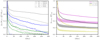Fig. A.1.

Left panel shows the time dependence of the physical fraction of stars in clusters (gray lines; the same as Figure 1) and the estimated observed fraction of stars in clusters when using r_search = 5 pc (blue lines) and r_search = 2 pc (green lines). The cluster mass is indicated by the line style. The right panel shows the time dependence of the physical fraction of stars in clusters (solid lines) and the estimated observed fraction of stars in clusters assuming r_search between 2 to 5 pc (filled areas). This panel is for the ECMF of Eq. (4) with β = 1.5 (magenta), β = 2 (black), and β = 2.4 (yellow).

All Tables

Table 1.

The fraction of stars in clusters ${\bar{f}}_{IC, pop} (t < 300 Myr)$ $\overline{f}_{\mathrm{IC,pop}} (t < 300\,\mathrm{Myr})$ for a time-independent SFR for stars younger than 300 Myr.

In the text

All Figures

	Fig. 1. Fraction of all stars that are present in their birth clusters at a given age, t, for clusters of initial mass M_ecl = 100 M_⊙ (dash-dotted line), M_ecl = 400 M_⊙ (dotted line), M_ecl = 1600 M_⊙ (dashed line), and M_ecl = 6400 M_⊙ (solid line).
In the text

	Fig. 2. Fraction of all stars located in their parent cluster for the galaxy-wide ECMF of Eq. (4) and for a single starburst. Clusters orbit the galaxy at R_g = 4 kpc, R_g = 8 kpc, and R_g = 12 kpc (different thickness of solid lines). These clusters have the Solar metallicity of Z = 0.014. Models of Z = 0.006 and Z = 0.002 for R_g = 8 kpc are shown by the dashed and dotted lines.
In the text

Fig. 3.

Time dependence of the fraction of M (red line), F-K (orange), A (yellow), late B (green), early B (blue), and O (magenta) stars located in clusters for clusters with R_g = 8 kpc and Z = 0.014. The clusters are assumed to form with the ECMF of Eq. (4) with β = 2, M_ecl, min = 30 M_⊙, and M_ecl, max = 10⁴ M_⊙. At a given time, f_IC, pop(m) increases with stellar mass (apart from O stars), which is the result of dynamically induced mass segregation. The O stars are slightly depleted in clusters because of their dynamical ejections.

In the text

Fig. 4.

Time dependence of the galaxy-wide f_IC, pop for galaxies with SFRs of 0.01 M_⊙ yr⁻¹, 0.1 M_⊙ yr⁻¹, 1 M_⊙ yr⁻¹, 10 M_⊙ yr⁻¹, and 100 M_⊙ yr⁻¹ (indicated by line colour) according to the IGIMF theory. The clusters have a metallicity of Z = 0.014 and orbit the galaxy at R_g = 8 kpc. The cluster mass range spans from 5 M_⊙ to M_ecl, max(SFR), which is given by Eq. (6). For each value of the SFR, we consider β = 1.5 (dashed lines), β = 2 (solid lines), and β = 2.4 (dotted lines).

In the text

Fig. 5.

Likely detected fraction of stars in clusters of age t < 10 Myr (blue area and blue lines), 10 Myr < t < 100 Myr (yellow area and yellow lines), and 100 Myr < t < 300 Myr (red area and red lines) as a function of Σ_SFR. Apart from indicating age by colour, age is also shown by a hatch style. The coloured area is bordered by two extreme models: the lower one has β = 2.2 and r_search = 2 pc, the upper one has β = 1.8 and r_search = 5 pc. The models for β = 2.0 and r_search = 2 pc and 5 pc are shown by the dashed lines. The plot shows how ${\bar{f}}_{IC, pop}^{obs}$ $\overline{f}^{\mathrm{obs}}_{\mathrm{IC,pop}}$ increases with the Σ_SFR, and how it decreases with the cluster age. The observational data from Chandar et al. (2017), which are aimed consistently at galaxies both with low SFR and high SFR, are shown by empty squares with their errorbars. Our results are obtained at almost the same time intervals as the observational data (indicated by the colours). The semi-analytic estimate provided by the Γ − Σ_SFR model is shown by the black solid line. We note its disagreement with the observational data for the clusters of any age interval.

In the text

	Fig. 6. Fraction of stars located in clusters of an initial mass M_ecl for ‘A’ models (blue lines) and ‘F’ models (magenta lines). For comparison, standard models are shown by red lines. The ‘A’ and ‘F’ models result in substantially lower fraction of stars in clusters of all considered masses at t ≳ 20 Myr.
In the text

Fig. 7.

Fraction of stars which is likely to be observed in clusters of age t < 10 Myr (blue lines), 10 Myr < t < 100 Myr (yellow lines), and 100 Myr < t < 300 Myr (red lines) as a function of Σ_SFR. The plot shows results for the ‘S’, ‘A’, and ‘F’ models for the ECMF of slope β = 2 by solid, dashed, and dotted lines, respectively. The lines are shown for r_search = 2 pc (smaller dots) and r_search = 5 pc (larger dots) for each model. The prediction of the Γ − Σ_SFR model and the observational data from Chandar et al. (2017) are shown by the black line and by squares, respectively.

In the text

Fig. 8.

Time dependence of f_IC(m) for clusters of mass 400 M_⊙ starting with initial conditions for models ‘S’ (solid lines) and ‘M’ (dashed lines). The values of f_IC(m) for different stellar spectral types is shown by line colours. The fraction of all stars in clusters f_IC(M_ecl = 400 M_⊙) is shown by the black lines. The clusters orbit the galaxy at R_g = 8 kpc and they have metallicity of Z = 0.014.

In the text

Fig. A.1.

Left panel shows the time dependence of the physical fraction of stars in clusters (gray lines; the same as Figure 1) and the estimated observed fraction of stars in clusters when using r_search = 5 pc (blue lines) and r_search = 2 pc (green lines). The cluster mass is indicated by the line style. The right panel shows the time dependence of the physical fraction of stars in clusters (solid lines) and the estimated observed fraction of stars in clusters assuming r_search between 2 to 5 pc (filled areas). This panel is for the ECMF of Eq. (4) with β = 1.5 (magenta), β = 2 (black), and β = 2.4 (yellow).

In the text

Current usage metrics show cumulative count of Article Views (full-text article views including HTML views, PDF and ePub downloads, according to the available data) and Abstracts Views on Vision4Press platform.

Data correspond to usage on the plateform after 2015. The current usage metrics is available 48-96 hours after online publication and is updated daily on week days.

Initial download of the metrics may take a while.

[1] Aarseth, S. J. 2003, Gravitational N-Body Simulations (Cambridge: Cambridge University Press) [Google Scholar]

[2] Aarseth, S. J., & Zare, K. 1974, Celest. Mech., 10, 185 [NASA ADS] [CrossRef] [Google Scholar]

[3] Adamo, A., Östlin, G., & Zackrisson, E. 2011, MNRAS, 417, 1904 [NASA ADS] [CrossRef] [Google Scholar]

[4] Ahmad, A., & Cohen, L. 1973, J. Comput. Phys., 12, 389 [Google Scholar]

[5] Allen, C., & Santillan, A. 1991, Rev. Mex. Astron. Astrofis., 22, 255 [NASA ADS] [Google Scholar]

[6] Alves, J., Lombardi, M., & Lada, C. J. 2007, A&A, 462, L17 [NASA ADS] [CrossRef] [EDP Sciences] [Google Scholar]

[7] André, P., Di Francesco, J., Ward-Thompson, D., et al. 2014, in Protostars and Planets VI, eds. H. Beuther, R. S. Klessen, C. P. Dullemond, & T. Henning, 27 [Google Scholar]

[8] Banerjee, S., & Kroupa, P. 2013, ApJ, 764, 29 [CrossRef] [Google Scholar]

[9] Banerjee, S., & Kroupa, P. 2015, MNRAS, 447, 728 [NASA ADS] [CrossRef] [Google Scholar]

[10] Banerjee, S., & Kroupa, P. 2017, A&A, 597, A28 [NASA ADS] [CrossRef] [EDP Sciences] [Google Scholar]

[11] Baumgardt, H., & Kroupa, P. 2007, MNRAS, 380, 1589 [NASA ADS] [CrossRef] [Google Scholar]

[12] Baumgardt, H., & Makino, J. 2003, MNRAS, 340, 227 [NASA ADS] [CrossRef] [Google Scholar]

[13] Bik, A., Lamers, H. J. G. L. M., Bastian, N., Panagia, N., & Romaniello, M. 2003, A&A, 397, 473 [CrossRef] [EDP Sciences] [Google Scholar]

[14] Blaauw, A. 1964, ARA&A, 2, 213 [Google Scholar]

[15] Boily, C. M., & Kroupa, P. 2003, MNRAS, 338, 673 [NASA ADS] [CrossRef] [Google Scholar]

[16] Bonnell, I. A., Bate, M. R., Clarke, C. J., & Pringle, J. E. 1997, MNRAS, 285, 201 [NASA ADS] [CrossRef] [Google Scholar]

[17] Bonnell, I. A., Bate, M. R., & Zinnecker, H. 1998, MNRAS, 298, 93 [Google Scholar]

[18] Bonnell, I. A., Bate, M. R., Clarke, C. J., & Pringle, J. E. 2001, MNRAS, 323, 785 [Google Scholar]

[19] Bressert, E., Bastian, N., Gutermuth, R., et al. 2010, MNRAS, 409, L54 [NASA ADS] [Google Scholar]

[20] Carpenter, J. M. 2000, AJ, 120, 3139 [Google Scholar]

[21] Carpenter, J. M., Snell, R. L., & Schloerb, F. P. 1995, ApJ, 450, 201 [NASA ADS] [CrossRef] [Google Scholar]

[22] Chandar, R., Fall, S. M., & Whitmore, B. C. 2010, ApJ, 711, 1263 [Google Scholar]

[23] Chandar, R., Fall, S. M., Whitmore, B. C., & Mulia, A. J. 2017, ApJ, 849, 128 [NASA ADS] [CrossRef] [Google Scholar]

[24] Chen, H. H.-H., Burkhart, B., Goodman, A., & Collins, D. C. 2018, ApJ, 859, 162 [NASA ADS] [CrossRef] [Google Scholar]

[25] Clark, P. C., Bonnell, I. A., Zinnecker, H., & Bate, M. R. 2005, MNRAS, 359, 809 [NASA ADS] [CrossRef] [Google Scholar]

[26] Colín, P., Vázquez-Semadeni, E., & Gómez, G. C. 2013, MNRAS, 435, 1701 [CrossRef] [Google Scholar]

[27] de la Fuente Marcos, R., & de la Fuente Marcos, C. 2004, New Astron., 9, 475 [NASA ADS] [CrossRef] [Google Scholar]

[28] Dib, S., & Henning, T. 2019, A&A, 629, A135 [NASA ADS] [CrossRef] [EDP Sciences] [Google Scholar]

[29] Dinnbier, F., & Walch, S. 2020, MNRAS, 499, 748 [Google Scholar]

[30] Domínguez, R., Fellhauer, M., Blaña, M., Farias, J. P., & Dabringhausen, J. 2017, MNRAS, 472, 465 [CrossRef] [Google Scholar]

[31] Elmegreen, B. G. 1983, MNRAS, 203, 1011 [NASA ADS] [CrossRef] [Google Scholar]

[32] Elmegreen, B. G. 2000, ApJ, 539, 342 [NASA ADS] [CrossRef] [Google Scholar]

[33] Elmegreen, B. G., Elmegreen, D. M., Chandar, R., Whitmore, B., & Regan, M. 2006, ApJ, 644, 879 [NASA ADS] [CrossRef] [Google Scholar]

[34] Er, X.-Y., Jiang, Z.-B., & Fu, Y.-N. 2013, Res. Astron. Astrophys., 13, 277 [CrossRef] [Google Scholar]

[35] Fall, S. M., Chandar, R., & Whitmore, B. C. 2005, ApJ, 631, L133 [NASA ADS] [CrossRef] [Google Scholar]

[36] Fensch, J., Duc, P.-A., Boquien, M., et al. 2019, A&A, 628, A60 [NASA ADS] [CrossRef] [EDP Sciences] [Google Scholar]

[37] Fujii, M. S., & Portegies Zwart, S. 2011, Science, 334, 1380 [Google Scholar]

[38] Gavagnin, E., Bleuler, A., Rosdahl, J., & Teyssier, R. 2017, MNRAS, 472, 4155 [NASA ADS] [CrossRef] [Google Scholar]

[39] Geen, S., Watson, S. K., Rosdahl, J., et al. 2018, MNRAS, 481, 2548 [CrossRef] [Google Scholar]

[40] Geyer, M. P., & Burkert, A. 2001, MNRAS, 323, 988 [NASA ADS] [CrossRef] [Google Scholar]

[41] Gieles, M., Larsen, S. S., Bastian, N., & Stein, I. T. 2006, A&A, 450, 129 [NASA ADS] [CrossRef] [EDP Sciences] [Google Scholar]

[42] Goddard, Q. E., Bastian, N., & Kennicutt, R. C. 2010, MNRAS, 405, 857 [NASA ADS] [Google Scholar]

[43] González-Samaniego, A., & Vazquez-Semadeni, E. 2020, MNRAS, 499, 668 [CrossRef] [Google Scholar]

[44] Goodwin, S. P. 1997, MNRAS, 284, 785 [Google Scholar]

[45] Goodwin, S. P., Nutter, D., Kroupa, P., Ward-Thompson, D., & Whitworth, A. P. 2008, A&A, 477, 823 [NASA ADS] [CrossRef] [EDP Sciences] [Google Scholar]

[46] Gvaramadze, V. V., Weidner, C., Kroupa, P., & Pflamm-Altenburg, J. 2012, MNRAS, 424, 3037 [NASA ADS] [CrossRef] [Google Scholar]

[47] Haid, S., Walch, S., Seifried, D., et al. 2018, MNRAS, 478, 4799 [Google Scholar]

[48] Heiderman, A., Evans, N. J., II, Allen, L. E., Huard, T., & Heyer, M. 2010, ApJ, 723, 1019 [Google Scholar]

[49] Heyer, M., Krawczyk, C., Duval, J., & Jackson, J. M. 2009, ApJ, 699, 1092 [Google Scholar]

[50] Hunter, J. D. 2007, Comput. Sci. Eng., 9, 90 [NASA ADS] [CrossRef] [Google Scholar]

[51] Hunter, D. A., Elmegreen, B. G., Dupuy, T. J., & Mortonson, M. 2003, AJ, 126, 1836 [NASA ADS] [CrossRef] [Google Scholar]

[52] Hurley, J. R., Pols, O. R., & Tout, C. A. 2000, MNRAS, 315, 543 [Google Scholar]

[53] Hurley, J. R., Tout, C. A., & Pols, O. R. 2002, MNRAS, 329, 897 [Google Scholar]

[54] Jerabkova, T., Boffin, H. M. J., Beccari, G., et al. 2021, A&A, 647, A137 [NASA ADS] [CrossRef] [EDP Sciences] [Google Scholar]

[55] Jeřábková, T., Hasani Zonoozi, A., Kroupa, P., et al. 2018, A&A, 620, A39 [Google Scholar]

[56] Johnson, L. C., Seth, A. C., Dalcanton, J. J., et al. 2016, ApJ, 827, 33 [NASA ADS] [CrossRef] [Google Scholar]

[57] Johnson, L. C., Seth, A. C., Dalcanton, J. J., et al. 2017, ApJ, 839, 78 [NASA ADS] [CrossRef] [Google Scholar]

[58] Joncour, I., Duchêne, G., Moraux, E., & Motte, F. 2018, A&A, 620, A27 [NASA ADS] [CrossRef] [EDP Sciences] [Google Scholar]

[59] Kennicutt, R. C., Jr. 1998, ApJ, 498, 541 [Google Scholar]

[60] Kirk, H., & Myers, P. C. 2011, ApJ, 727, 64 [Google Scholar]

[61] Kritsuk, A. G., Norman, M. L., & Wagner, R. 2011, ApJ, 727, L20 [NASA ADS] [CrossRef] [Google Scholar]

[62] Kroupa, P. 1995a, MNRAS, 277, 1507 [NASA ADS] [Google Scholar]

[63] Kroupa, P. 1995b, MNRAS, 277, 1491 [Google Scholar]

[64] Kroupa, P. 2001, MNRAS, 322, 231 [NASA ADS] [CrossRef] [Google Scholar]

[65] Kroupa, P., & Bouvier, J. 2003, MNRAS, 346, 343 [NASA ADS] [CrossRef] [Google Scholar]

[66] Kroupa, P., & Weidner, C. 2003, ApJ, 598, 1076 [NASA ADS] [CrossRef] [Google Scholar]

[67] Kroupa, P., Aarseth, S., & Hurley, J. 2001, MNRAS, 321, 699 [NASA ADS] [CrossRef] [Google Scholar]

[68] Kruijssen, J. M. D. 2012, MNRAS, 426, 3008 [Google Scholar]

[69] Kuhn, M. A., Feigelson, E. D., Getman, K. V., et al. 2014, ApJ, 787, 107 [Google Scholar]

[70] Kuhn, M. A., Hillenbrand, L. A., Sills, A., Feigelson, E. D., & Getman, K. V. 2019, ApJ, 870, 32 [CrossRef] [Google Scholar]

[71] Küpper, A. H. W., Maschberger, T., Kroupa, P., & Baumgardt, H. 2011, MNRAS, 417, 2300 [Google Scholar]

[72] Kustaanheimo, P., & Stiefel, E. 1965, Reine Angew. Math., 218, 204 [Google Scholar]

[73] Lada, C. J., & Lada, E. A. 2003, ARA&A, 41, 57 [Google Scholar]

[74] Lada, C. J., Margulis, M., & Dearborn, D. 1984, ApJ, 285, 141 [NASA ADS] [CrossRef] [Google Scholar]

[75] Lada, E. A., Depoy, D. L., Evans, N. J., II, & Gatley, I. 1991, ApJ, 371, 171 [NASA ADS] [CrossRef] [Google Scholar]

[76] Lada, C. J., Lombardi, M., & Alves, J. F. 2009, ApJ, 703, 52 [NASA ADS] [CrossRef] [Google Scholar]

[77] Lada, C. J., Lombardi, M., & Alves, J. F. 2010, ApJ, 724, 687 [Google Scholar]

[78] Lamers, H. J. G. L. M., & Gieles, M. 2006, A&A, 455, L17 [NASA ADS] [CrossRef] [EDP Sciences] [Google Scholar]

[79] Lamers, H. J. G. L. M., Gieles, M., Bastian, N., et al. 2005, A&A, 441, 117 [NASA ADS] [CrossRef] [EDP Sciences] [Google Scholar]

[80] Larsen, S. S. 2002, AJ, 124, 1393 [NASA ADS] [CrossRef] [Google Scholar]

[81] Larson, R. B. 1981, MNRAS, 194, 809 [Google Scholar]

[82] Leinert, C., Zinnecker, H., Weitzel, N., et al. 1993, A&A, 278, 129 [NASA ADS] [Google Scholar]

[83] Lombardi, M., Alves, J., & Lada, C. J. 2015, A&A, 576, L1 [NASA ADS] [CrossRef] [EDP Sciences] [Google Scholar]

[84] Lüghausen, F., Parmentier, G., Pflamm-Altenburg, J., & Kroupa, P. 2012, MNRAS, 423, 1985 [CrossRef] [Google Scholar]

[85] Makino, J. 1991, ApJ, 369, 200 [Google Scholar]

[86] Makino, J., & Aarseth, S. J. 1992, PASJ, 44, 141 [NASA ADS] [Google Scholar]

[87] Marks, M., & Kroupa, P. 2011, MNRAS, 417, 1702 [NASA ADS] [CrossRef] [Google Scholar]

[88] Marks, M., & Kroupa, P. 2012, A&A, 543, A8 [NASA ADS] [CrossRef] [EDP Sciences] [Google Scholar]

[89] Mason, B. D., Gies, D. R., Hartkopf, W. I., et al. 1998, AJ, 115, 821 [NASA ADS] [CrossRef] [Google Scholar]

[90] Megeath, S. T., Gutermuth, R., Muzerolle, J., et al. 2016, AJ, 151, 5 [Google Scholar]

[91] Mikkola, S., & Aarseth, S. J. 1990, Celest. Mech. Dyn. Astron., 47, 375 [CrossRef] [Google Scholar]

[92] Oh, S., & Kroupa, P. 2016, A&A, 590, A107 [NASA ADS] [CrossRef] [EDP Sciences] [Google Scholar]

[93] Oh, S., Kroupa, P., & Pflamm-Altenburg, J. 2015, ApJ, 805, 92 [Google Scholar]

[94] Padoan, P., Nordlund, A., & Jones, B. J. T. 1997, MNRAS, 288, 145 [NASA ADS] [CrossRef] [Google Scholar]

[95] Pang, X., Li, Y., Tang, S.-Y., Pasquato, M., & Kouwenhoven, M. B. N. 2020, ApJ, 900, L4 [NASA ADS] [CrossRef] [Google Scholar]

[96] Perets, H. B., & Šubr, L. 2012, ApJ, 751, 133 [Google Scholar]

[97] Pfalzner, S. 2019, Proc. IAU Symp., 14, 208 [NASA ADS] [CrossRef] [Google Scholar]

[98] Pflamm-Altenburg, J., & Kroupa, P. 2008, Nature, 455, 641 [Google Scholar]

[99] Plunkett, A. L., Fernández-López, M., Arce, H. G., et al. 2018, A&A, 615, A9 [NASA ADS] [CrossRef] [EDP Sciences] [Google Scholar]

[100] Porras, A., Christopher, M., Allen, L., et al. 2003, AJ, 126, 1916 [NASA ADS] [CrossRef] [Google Scholar]

[101] Portegies Zwart, S. F., McMillan, S. L. W., & Gieles, M. 2010, ARA&A, 48, 431 [NASA ADS] [CrossRef] [Google Scholar]

[102] Preibisch, T., & Zinnecker, H. 1999, AJ, 117, 2381 [NASA ADS] [CrossRef] [Google Scholar]

[103] Randriamanakoto, Z., Escala, A., Väisänen, P., et al. 2013, ApJ, 775, L38 [NASA ADS] [CrossRef] [Google Scholar]

[104] Reipurth, B., & Zinnecker, H. 1993, A&A, 278, 81 [NASA ADS] [Google Scholar]

[105] Rogers, H., & Pittard, J. M. 2013, MNRAS, 431, 1337 [CrossRef] [Google Scholar]

[106] Röser, S., & Schilbach, E. 2019, A&A, 627, A4 [NASA ADS] [CrossRef] [EDP Sciences] [Google Scholar]

[107] Röser, S., Schilbach, E., Piskunov, A. E., Kharchenko, N. V., & Scholz, R. D. 2011, A&A, 531, A92 [NASA ADS] [CrossRef] [EDP Sciences] [Google Scholar]

[108] Sana, H., de Mink, S. E., de Koter, A., et al. 2012, Science, 337, 444 [Google Scholar]

[109] Schmidt, M. 1959, ApJ, 129, 243 [NASA ADS] [CrossRef] [Google Scholar]

[110] Schneider, N., André, P., Könyves, V., et al. 2013, ApJ, 766, L17 [NASA ADS] [CrossRef] [Google Scholar]

[111] Selier, R., Heydari-Malayeri, M., & Gouliermis, D. A. 2011, A&A, 529, A40 [NASA ADS] [CrossRef] [EDP Sciences] [Google Scholar]

[112] Spera, M., & Capuzzo-Dolcetta, R. 2017, Ap&SS, 362, 233 [NASA ADS] [CrossRef] [Google Scholar]

[113] Stephens, I. W., Gouliermis, D., Looney, L. W., et al. 2017, ApJ, 834, 94 [Google Scholar]

[114] Stone, R. C. 1991, AJ, 102, 333 [NASA ADS] [CrossRef] [Google Scholar]

[115] Tanikawa, A., Hut, P., & Makino, J. 2012, New Astron., 17, 272 [NASA ADS] [CrossRef] [Google Scholar]

[116] Terlevich, E. 1987, MNRAS, 224, 193 [NASA ADS] [CrossRef] [Google Scholar]

[117] Tetzlaff, N., Neuhäuser, R., & Hohle, M. M. 2011, MNRAS, 410, 190 [Google Scholar]

[118] Tout, C. A., Pols, O. R., Eggleton, P. P., & Han, Z. 1996, MNRAS, 281, 257 [Google Scholar]

[119] Tutukov, A. V. 1978, A&A, 70, 57 [NASA ADS] [Google Scholar]

[120] van den Bergh, S., & Lafontaine, A. 1984, AJ, 89, 1822 [NASA ADS] [CrossRef] [Google Scholar]

[121] Vazquez-Semadeni, E. 1994, ApJ, 423, 681 [Google Scholar]

[122] Šubr, L., Kroupa, P., & Baumgardt, H. 2008, MNRAS, 385, 1673 [CrossRef] [Google Scholar]

[123] Wang, L., Spurzem, R., Aarseth, S., et al. 2015, MNRAS, 450, 4070 [NASA ADS] [CrossRef] [Google Scholar]

[124] Wang, L., Kroupa, P., & Jerabkova, T. 2019, MNRAS, 484, 1843 [NASA ADS] [CrossRef] [Google Scholar]

[125] Wang, L., Iwasawa, M., Nitadori, K., & Makino, J. 2020, MNRAS, 497, 536 [NASA ADS] [CrossRef] [Google Scholar]

[126] Weidner, C., Kroupa, P., & Larsen, S. S. 2004, MNRAS, 350, 1503 [CrossRef] [Google Scholar]

[127] Weidner, C., Kroupa, P., & Bonnell, I. A. D. 2010, MNRAS, 401, 275 [NASA ADS] [CrossRef] [Google Scholar]

[128] Weidner, C., Kroupa, P., & Pflamm-Altenburg, J. 2013, MNRAS, 434, 84 [NASA ADS] [CrossRef] [Google Scholar]

[129] Whitmore, B. C., Zhang, Q., Leitherer, C., et al. 1999, AJ, 118, 1551 [CrossRef] [Google Scholar]

[130] Whitmore, B. C., Chandar, R., & Fall, S. M. 2007, AJ, 133, 1067 [NASA ADS] [CrossRef] [Google Scholar]

[131] Winston, E., Hora, J. L., & Tolls, V. 2020, AJ, 160, 68 [NASA ADS] [CrossRef] [Google Scholar]

[132] Yan, Z., Jerabkova, T., & Kroupa, P. 2017, A&A, 607, A126 [NASA ADS] [CrossRef] [EDP Sciences] [Google Scholar]

[133] Zinnecker, H., & Yorke, H. W. 2007, ARA&A, 45, 481 [Google Scholar]