| Issue |
A&A
Volume 660, April 2022
|
|
|---|---|---|
| Article Number | A62 | |
| Number of page(s) | 6 | |
| Section | Stellar structure and evolution | |
| DOI | https://doi.org/10.1051/0004-6361/202141544 | |
| Published online | 13 April 2022 | |
Speed of sound in dense matter and two families of compact stars
1
Dipartimento di Fisica e Scienze della Terra, Università di Ferrara, Via Saragat 1, 44122 Ferrara, Italy
2
INFN Sezione di Ferrara, Via Saragat 1, 44122 Ferrara, Italy
3
Space Sciences, Technologies and Astrophysics Research (STAR) Institute, Université de Liège, Bât. B5a, 4000 Liège, Belgium
e-mail: This email address is being protected from spambots. You need JavaScript enabled to view it.
Received:
14
June
2021
Accepted:
9
January
2022
Abstract
The existence of massive compact stars (M ≳ 2.1 M⊙) implies that the speed of sound exceeds the conformal limit (cs2 = 1/3 × the squared speed of light in vacuum) if those stars have an inner and outer crust of ordinary nuclear matter. Here, we show that if the most massive objects are strange quark stars, namely, stars entirely composed of quarks, cs can assume values below the conformal limit even while observational limits on those objects are also satisfied. By using astrophysical data associated with those massive stars derived from electromagnetic and gravitational wave signals, we use a Bayesian analysis framework and by adopting a constant speed of sound equation of state to show that the posterior distribution of cs2 is peaked around 0.3 and the maximum mass of the most probable equation of state is ∼2.13 M⊙. We discuss which new data would require a speed of sound larger than the conformal limit even when considering strange quark stars. In particular, we analyze the possibility that the maximum mass of compact stars is larger than 2.5 M⊙, as it would be if the secondary component of GW190814 would turn out to be a compact star – and not a black hole, as previously assumed. Finally, we discuss how the new data for PSR J0740+6620 obtained by the NICER collaboration compare with our results and find they are in qualitative agreement. We conclude with a brief discussion of other possible interpretations of our analysis.
Key words: dense matter / equation of state / stars: neutron
© ESO 2022
1. Introduction
Following the discovery of neutron stars with masses of ∼2 M⊙ (Demorest et al. 2010; Antoniadis et al. 2013; Cromartie et al. 2019), it became clear that the equation of state (EoS) of dense baryonic matter must be rather stiff to support such a large mass against gravitational collapse. The stiffness of the equation of state for nucleonic matter is regulated by the adiabatic index or, equivalently, by the speed of sound, cs, the derivative of pressure with respect to the energy density at fixed entropy. A remarkable result obtained in Bedaque & Steiner (2015) (also see the more recent work by Reed & Horowitz 2020) is that while it is expected that at an asymptotically high density, the speed of sound must respect the conformal limit of  1, due to the QCD asymptotic freedom at the densities reached in the core of neutron stars, this limit does not apply; thus: cs must increase to values significantly larger than the conformal bound and then it should decrease to asymptotically reach the conformal limit. In particular, if we assume that compact stars have an external layer of ordinary nuclear matter up to a density of ρc ∼ 2ρ0 (where ρ0 is the nuclear matter saturation density) and that at densities of ρ > ρc, matter has a constant speed of sound,
  , then we realize that masses of ∼2 M⊙ cannot be obtained (Bedaque & Steiner 2015). If we instead matche the external layer and core at ∼1.1ρ0, masses up to 2 M⊙ can be obtained, but not any greater (Annala et al. 2020). While this need to exceed the conformal limit stems from the assumption that the mass of a star with a ordinary crust exceeds ∼2 M⊙, larger values of cs are requested if conditions on the radii are also imposed. For instance, in order to obtain radii smaller than about 12 km for masses about (1.4−1.5) M⊙, we can assume that a phase transition takes place at some density larger than ρ0, obtaining stars having a core of quark matter separated, via a large energy density jump, from a nucleonic layer. Small radii can then be obtained in particular in the so-called twin stars model (Alvarez-Castillo & Blaschke 2017; Christian & Schaffner-Bielich 2020; Blaschke et al. 2020), but only if cs is set to be very close to the causal limit cs = 1 (Chamel et al. 2013; Alford et al. 2013, 2015). We note that this inferred behaviour for cs is different from what happens at finite temperature and zero density matter, where a lattice QCD has definitively established that cs is always below the conformal limit (Karsch 2007), a behaviour that is predicted also in several weak couplings and strong couplings theories (for more, see Bedaque & Steiner 2015).
The density in the core of neutron stars (with values up to 10ρ0) is clearly shown to be far below the densities at which pQCD can be applied, that is, at densities larger than ∼40ρ0 (Komoltsev & Kurkela 2021). Thus, there is no tension between the existence of massive stars and the need to recover the high density conformal limit. Indeed one can imagine that there is some physical mechanism which is responsible for a rapid increase of cs at densities close to twice saturation density and which then “switches off” at high densities. At those densities, cs should decrease again below the conformal limit and then reach it asymptotically from below, which is in agreement with pQCD calculations. There are several examples in the literature for this kind of explanation (see Hoyos et al. 2016; Tews et al. 2018; Ma & Rho 2019; Khaidukov & Simonov 2018; McLerran & Reddy 2019; Marczenko 2020).
On the other hand, it is also possible that cs does not need to exceed the conformal limit at neutron stars densities because two types of stars exist: hadronic stars (HSs) and strange quark stars (QSs) as described by the so-called two-families scenario (Drago et al. 2014a, 2016; Drago & Pagliara 2018; Char et al. 2019; De Pietri et al. 2019). In that scenario, the most massive stars are QSs and (as shown in the present paper), the conformal limit can be respected even if the maximum mass exceeds 2 M⊙.
Strange quark stars are self-bound objects having a profile which ends at the surface of the star with a finite (and large) value of the energy density, e0, of the order of that of nuclear matter at saturation. It is well known that for this kind of objects, the maximum mass does depend on the speed of sound, as in the case of ordinary neutron stars, but also on the value of e0. In particular, when adopting the most simple prescription, namely, the constant speed of sound (CSS) EoS  , where p and e are pressure and energy density (Alford et al. 2013; Zdunik & Haensel 2013; Chamel et al. 2013; Drago et al. 2019)2, can show that the maximum mass
  (Lattimer & Prakash 2011). Unfortunately, there no such simple scaling with cs exists. We numerically computed the maximum mass (often called Tolman–Oppenheimer–Volkoff mass) as a function of cs and e0 and found the following parametrization: mmax(x, e0)=(en/e0)1/2(0.11 + 3.27x − 1.04x2 + 0.13x3), where
  and en = 150 MeV fm)−3 represent the nuclear matter energy density at saturation. This parametrization has been found to be a rather good approximation of the numerical results in the range 0.1 ≤ cs ≤ 1 (the dependence on e0 is instead analytical and therefore exact). We display in Fig. 1 the contour plot of mmax. We may notice that in the conformal limit, x = 1, it is possible to reach the range 2 M⊙ ≲ mmax ≲ 2.5 M⊙ provided that 1 ≲ e0/en ≲ 1.5. Thus, cs does not need to exceed the conformal limit in order to have masses larger than 2 M⊙ when QSs are considered. Actually, we may also notice from the same plot that even a value of x as low as x ∼ 0.75 allows for mmax ∼ 2 M⊙ to be reached, provided that e0 coincides with the nuclear matter density, en. While such a low value of e0 is probably unrealistic, this result indicates that there is a window of values for cs and e0 that allows us to obtain massive stars – even when cs is well below the conformal limit. Indeed, in Dondi et al. (2017), by adopting the chiral color dielectric model for computing the EoS of quark matter, it was found that it is possible to obtain values of mmax close to the 2 M⊙ limit when cs approaches the conformal limit from below. Thus, within the two families scenario, it is not necessary to have values of cs larger than the conformal limit – at least for masses not exceeding ∼2.5 M⊙.
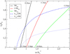 |
Fig. 1. Contour plot for mmax. Solid lines show the curves of constant maximum mass in the parameter space of the CSS model. At the beginning and at the end of those lines, the radii corresponding to the maximum mass configurations are also indicated. The vertical dotted line indicates the conformal limit. The blue dashed and dotted lines are curves of constant Λ1.6, for the two values Λ1.6 = 250 and 500, which are close to the 68% and 90% confidence interval obtained from the analysis of GW170817 (see Fig. 3). |
A correlated issue concerns the radii of QSs. We can show that the radius of the maximum mass configuration scales as rmax(x, e0) = (en/e0)1/2(7.06 + 9.40x − 3.42x2 + 0.47x3). In Fig. 1, we indicate the range of values of rmax for fixed values of mmax. Clearly, the larger the value of mmax, the greater the value of rmax (which reaches ∼15 km for e0/en = 1 and mmax = 3 M⊙). In the two-families scenario, it is therefore natural to interpret stars with large radii as massive QSs. This will be the starting point of the discussion on the astrophysical data presented in Sect. 2.
In our analysis, we consider bare QSs, namely, stars with a sharp discontinuity at the surface. On the other hand, QSs can have a crust made of ordinary nuclear matter, suspended over their bare surface due to a strong electric field, which is a feature that has been investigated since the first seminal papers (see e.g., Haensel et al. 1986). We notice that for a QS having a mass of 1.4 M⊙, the thickness of the crust does not exceed 300 m and the mass is smaller than 1.7 × 10⁻⁵ M⊙ (Haensel et al. 2007). Moreover, the thickness and mass of the crust decrease for larger masses of the QS and, in our scenario, QSs are objects with a mass larger than about 1.45 M⊙. However, this tiny and light crust could be sufficient for explaining the X-ray phenomenology associated with the accretion of matter onto the stellar surface, evidenced by X-ray bursts. In particular, the quiescent luminosity of those accreting objects is generally thought to be powered by the deposition of heat in the crust, as discussed in Brown & Cumming (2009), (see also Chamel et al. 2020). Another possible crust-like scenario is based on the existence of a color superconducting crystalline phase, forming an envelop around the fluid quark core (see Anglani et al. 2014). We notice that the crystalline phase crust and the ordinary nuclear matter crust suspended over the bare quark surface are not mutually exclusive. Indeed, also in the color superconducting crystalline phase, the electron fraction is finite (see Casalbuoni et al. 2005), the electrons sphere would extend over a length scale of ∼100 fm above the surface of the quark star and would lead to the formation of the strong electric field mentioned before Haensel et al. (2007). Thus, the X-ray phenomenology could also be explained in this case. The relevance of that crystalline envelop for other compact stars properties will be discussed later in this paper.
Finally, concerning HSs: as shown in Bedaque & Steiner (2015), they can reach mmax ∼ 1.9 M⊙ without exceeding the conformal limit. In fact, the formation of hyperons and delta resonances reduces the value of cs in hadronic matter with a consequent reduction of the values of the maximum mass and of the radii of HSs. Therefore, very compact HSs, with R1.4 ≲ 11 km (Burgio et al. 2018), can exist in the two-families scenario together with very massive QSs (Drago et al. 2014a), while having values of cs below the conformal limit both in the hadronic and in the quark sector.
The previous simple theoretical analysis establishes the possible values of mmax in the two-families scenario (by adopting the CSS model for quark matter). Those predictions need to be confronted with the available astrophysical data. It is the aim of this work to obtain the posterior distributions of e0 and cs by performing a Bayesian analysis on a selected sample of data that are interpreted as QSs within the two-families scenario. In our analysis, we did not use the recent data obtained by NICER on MSP J0740+6620 (Riley et al. 2021b; Miller et al. 2021b); instead, the estimate of the radius of an object having a mass ∼2.05 M⊙ (as in the case of MSP J0740+6620 Cromartie et al. 2019; Fonseca et al. 2021) is meant to be a relevant outcome of our analysis. Finally, we go on to discuss the possibility that the source of GW190814 (Abbott et al. 2020b) is a BH-CS system, implying that mmax is larger than 2.5 M⊙.
2. Selection of the sources
The two-families scenario is based on the coexistence of two classes of CSs. The first one, based on a soft hadronic EoS (Drago et al. 2014b), is composed of light and very compact HSs, with R1.4 on the order of (10.5−11) km and the second one by massive QSs with larger radii (Drago et al. 2014a, 2016). The formation of new degrees of freedom within HSs softens the EoS leading to a maximum mass  of ∼(1.5−1.6) M⊙. For the same baryonic mass, QSs have a gravitational mass lower than the one of HSs, on the order of 0.1 M⊙ or more (De Pietri et al. 2019) and, thus, the transition from HSs to QSs is strongly exothermic (Berezhiani et al. 2003; Bombaci et al. 2004, 2007; Drago et al. 2004; Drago & Pagliara 2020). The process of transformation of a HS into a QS can start only when there are enough hyperons at the center of the HS to form the first stable droplet of strange quark matter that can then trigger the conversion (see Drago et al. 2007; Herzog & Ropke 2011; Pagliara et al. 2013; Drago & Pagliara 2015). In turn, this implies the existence of a minimum mass for the QSs branch (if QSs generate from the conversion of a HS),
  and the coexistence of both HSs and QSs in the interval
 ![Mathematical equation: $ [m_{\mathrm{min}}^{\mathrm{QS}},m_{\mathrm{max}}^{\mathrm{HS}}] $](/articles/aa/full_html/2022/04/aa41544-21/aa41544-21-eq10.gif) . In this range, HSs and QSs can have the same mass but different radii.
. In this range, HSs and QSs can have the same mass but different radii.
We use the simultaneous measurements of masses and radii for several X-ray sources, as well as the masses and tidal deformabilities derived from the gravitational wave events reported by the LIGO-VIRGO collaboration (LVC; Aasi et al. 2015; Acernese et al. 2015). Specifically, for our sample of possible QSs candidates, we chose 4U 1724–207, SAX J1748.9 2021, 4U 1820–30, 4U 1702–429, J0437–4715 (Özel et al. 2016; Nättilä et al. 2017; Gonzalez-Caniulef et al. 2019), the high-mass component of GW170817 (Abbott et al. 2017, 2018), and both the components of GW190425 (Abbott et al. 2020a). For 4U 1702–429 (Nättilä et al. 2017) and J0437–4715 (Gonzalez-Caniulef et al. 2019), we took a bivariate Gaussian distribution to resemble the M − R posterior since the full distribution is not available. For all the other sources, we directly used the posterior distributions, which are publicly available. Our data refer to CSs that can be interpreted, within the two-families scenario, as being QSs (as we explain in the following).
Here, we clarify how we have chosen the sources in our analysis on the EoS of QSs. First, we classify J0437–4715 as a QS because its radius is larger than ∼13 km, the central value of its mass is ∼1.45 M⊙ and HSs in the two-families scenario cannot have such a large radius for that value of mass. We want to remark at this point that generally within the standard one-family scenario, HSs can be shown to have such large radii if the EoS is assumed to be stiff (see Fattoyev et al. 2018). However, the observational indications of objects with very small radii (see e.g., the analyses by Steiner et al. 2018 and Baillot d’Etivaux et al. 2019) that lead to R1.4 ≲ 12 km suggest a tension between different measurements. The two-families scenario solves this tension by assuming that HSs can be very compact due to softening of the EoS that is related to the appearance of delta resonances and hyperons (see Drago et al. 2014a).
For our analysis, we also chose the mass value of J0437–4715 as a guess for  . Thus,
  is fixed to
  and all the sources with masses of ≳1.55 M⊙ can be interpreted as QSs. In our analysis, the masses have been chosen as the mean values of the marginalized distribution of the sources. This criterion is fulfilled by all the sources that we selected in this study apart from GW170817_1, whose mass (∼1.49 M⊙) falls in the coexistence region
 ![Mathematical equation: $ [m_{\mathrm{min}}^{\mathrm{QS}},m_{\mathrm{max}}^{\mathrm{HS}}] $](/articles/aa/full_html/2022/04/aa41544-21/aa41544-21-eq14.gif) . The reason for assuming that GW170817_1 is a QS is phenomenological: the presence of strong electromagnetic counterparts associated with GW170817 (GRB170817A and AT2017gfo) implies that the merger event did not produce a prompt collapse. Since the threshold mass for a prompt collapse for a HS–HS binary has been estimated in De Pietri et al. (2019) as mthr = 2.5 M⊙, that event cannot be interpreted as a HS–HS merger within the two-families scenario and it must be classified as HS–QS merger. Thus, the heaviest component, GW170817_1, within the two-families scenario, is most probably a QS.
. The reason for assuming that GW170817_1 is a QS is phenomenological: the presence of strong electromagnetic counterparts associated with GW170817 (GRB170817A and AT2017gfo) implies that the merger event did not produce a prompt collapse. Since the threshold mass for a prompt collapse for a HS–HS binary has been estimated in De Pietri et al. (2019) as mthr = 2.5 M⊙, that event cannot be interpreted as a HS–HS merger within the two-families scenario and it must be classified as HS–QS merger. Thus, the heaviest component, GW170817_1, within the two-families scenario, is most probably a QS.
3. Results of the Bayesian analysis
Here, we present the results of our Bayesian analysis on the sources discussed in Sect. 2. We used the CSS parameterized EoS described before, with two free parameters: e0 and  . We selected the priors based on the assumption, for e0, of a flat distribution in the range between 160−232 MeV fm−3 and for
  , a flat distribution in the range [0.1, 1]. We set
  , which has obvious consequences with regard to the ranges of the parameters. Indeed, because of that constraint, in Traversi & Char (2020), the prior range for e0 was restricted to be e0 < 220 MeV fm−3 since
  was fixed to 1/3. This restriction no longer holds in the present two-parameters analysis, since an increase in
  allows for larger values of e0. Still, we note that we must have
  in order to reach 2 M⊙, as shown in Fig. 1. Details of this analysis, along with a comparison with the neural network-based prediction techniques, can be found in Traversi & Char (2020).
Next, we constructed the joint posterior and investigate the conformal limit on cs given the present data. We used the publicly available posterior samples of X-ray measurements from Özel et al. (2016)3 while the mass and tidal deformability samples of the binary merger components are provided by LVC4.
In Fig. 2, we display the marginalized PDFs for e0 and  along with their most probable values and the 1σ errors, and the 2D distribution with 1σ (39.3%), and 90% credible interval (CI). The quantiles are not directly useful to our analysis, but they indicate the trends in the posteriors. The region with larger likelihood corresponds to lower values of
  with corresponding not-too-large values of e0. Indeed, a positive correlation among these two parameters is found inside the 1σ region. The most probable point of the joint PDF is represented as a blue circle in Fig. 2 and it is located at e0 = 183.48 MeV fm−3, with
  . This is a remarkable result, namely: by adopting the two-families scenario and by performing a Bayesian analysis on the QSs candidates, we find that the preferred values of cs are not only far from the causal limit, but even values above the conformal limit seem to be unnecessary. We also note that this result cannot be reduced to the more trivial assumption that it is possible to reach large masses with QSs without adopting values of cs above the conformal limit. As shown in Fig. 1, if the observed radii were smaller, then values of
  greater than 1/3 would be necessary (at least with the rather trivial CSS EoS adopted here). Instead, we have demonstrated that: (1) the conformal limit can be respected even at neutron stars densities, with an EoS allowing for the existence of QSs because the radii are rather large; (2) for the observed values of masses and radii, the solution respecting the conformal limit is not only possible – but it may even be the most probable.
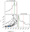 |
Fig. 2. Posterior for e0 and |

The M − R and M − Λ curves corresponding to the 68% CI are shown in Fig. 3. The higher likelihood region of the 2D posterior is associated to EoSs that are characterized by values of mmax in the range of ∼2.1−2.2 M⊙ and radii in the interval of R1.6 ∼ 11.6−12.9 km. We obtained for the most probable solution mmax = 2.13 M⊙ and R1.6 = 12.20 km. The corresponding curves in both panels in Fig. 3 are represented with a black dashed line. While the present work was in progress, the mass (and the distance) of J0740+6620 was measured again using radio data (Fonseca et al. 2021) and, in addition, X-ray observations by NICER constrained its mass-radius relation (Riley et al. 2021b; Miller et al. 2021b). These latest results are not included in our analysis, but they are shown in Fig. 3 together with the outcome of our Bayesian analysis, where it is possible to appreciate that our results are completely consistent with these new findings. Concerning the three tidal deformabilities of the stars included in our sample, it is clear that while there is a good agreement with the two components of GW190425, for GW170817_1, there is no overlap between the theoretical curves and the posterior distribution at the 68% CI. However at 90% CI the agreement is met also with GW170817_1 (see the blue dashed line of Fig. 3, right panel). The same argument goes for the object J0437−4715 in M − R plot, we find that our theoretical curves are matched at 90% CI – and not at 68%. So, our “best” curve is a little too stiff for GW170817 and a little too soft for J0437−4715, if they are both taken at 68%. We note that another Bayesian analysis performed by using similar sources by Fasano et al. (2019), although in the context of hadronic stars, the obtained radii are comparable to our best-fit curve. This may suggest a mild disagreement between two measurements, but might not be attributed to the choice of EoS model.
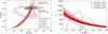 |
Fig. 3. Inferred M − R (left) and M − Λ (right) curves for the 68% CI corresponding to the EOS posterior along with the sources also at 68% (solid lines). The light blue and green patches correspond to the latest mass and radius measurements of the pulsar J0740+6620 (Fonseca et al. 2021; Riley et al. 2021a; Miller et al. 2021a). The black dashed lines represent the most probable EOS. The brown dashed curve on the left panel denotes the 90% of J0437–4715. Additionally, the blue dashed curve on the right panel denotes the 90% of the heavier component of GW170817. |
4. Considering whether GW190814 has a 2.6 M⊙ compact star component
The detection of the gravitational waves signal GW190814 by the LVC collaboration (Abbott et al. 2020b) led to the discovery of a binary system made of a 23 M⊙ BH and a CS companion of ∼2.6 M⊙ (the lower value at 90% credible level being 2.5 M⊙). The nature of the companion is rather uncertain since its mass falls within the BH lower mass gap but, on the other hand, such a massive neutron star challenges previous astronomical constraints and nuclear physics constraints (Fattoyev et al. 2020). In the recent work by Bombaci et al. (2021), it has been proposed that the companion could actually be a QS.
From the discussion presented in Sect. 1, it is clear that to explain the existence of a QS with M = 2.6 M⊙, we must also consider values of cs above the conformal limit in dense quark matter as well. That is to say that it is necessary, across a certain range of densities for  to be larger than 1/3. Alternatively, we should find a physical mechanism that reduces the value of e0. In Bombaci et al. (2021), this requirement is achieved by assuming that quark matter could be in a color superconducting state, namely, the CFL phase. The pressure, P, in this case is expressed as:
  , where Δ is the superconducting gap, μ the quark chemical potential, and ms the strange quark mass Alford et al. (2005). The additional term, proportional to
  , introduces a density dependence of cs, as shown in Fig. 4, and it also modifies the value of e0. In particular, if Δ > ms/2, then cs approaches the conformal limit from above and the value of e0 is reduced. In this way, it is possible to reach values of mmax larger than 2.5 M⊙, as shown in Bombaci et al. (2021), and to pin down a physical mechanism for explaining how cs can overcome the conformal bound at low densities. Still, we notice that the deviation from the conformal limit is rather small. Actually, the most important effect of the superconducting gap on the value of the maximum mass is derived from the reduction of e0 which, in this numerical example, is only slightly larger than en, namely, e0 = 152 MeV fm−3. For the same set of parameters (see, the caption of the figure), but with Δ = 0, we may obtain e0 = 190 MeV fm−3.
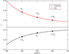 |
Fig. 4. Speed of sound as a function of the quark chemical potential μ for unpaired quark matter and CFL matter. For the latter, we use ms = 100, Δ = 80 MeV, B1/4 = 135 MeV, and the pQCD correction parameter is a4 = 0.7 (for details, see the main text). The dots on the two lines indicate the corresponding baryon densities in units of the nuclear density, nn. |
In conclusion, we can ask to what extent deviations from the conformal limit, within the two-families scenario, are necessary for the case where mmax > 2.5 M⊙. It clearly depends on how compact or (tidal deformable) QSs are. In Fig. 1, we display the 68% and 90% credible interval for the tidal deformability Λ of a 1.6 M⊙ star obtained from the analysis of GW170817: Λ1.6 ≲ 250 and Λ1.6 ≲ 500 (see also Fig. 3, right panel). Those constraints can be satisfied if 1.2 ≲ x ≲ 1.6, which is a deviation from the conformal limit but one that is still significantly smaller than what is needed in the case of hybrid stars (see Xie & Li 2021).
5. Conclusions
In this paper, we argue that the existence of massive compact stars, with masses up to 2.5 M⊙, does not necessarily imply that the speed of sound in dense strongly interacting matter exceeds the conformal limit, in agreement with the results of Lattimer & Prakash (2011). However, we have had to abandon the assumption that only one family of compact stars exists and assume that two separated branches in the mass–radius plot are possible: the HS branch and the QS branch. Within the two-families scenario, some astrophysical sources can be (with a certain degree of uncertainty) identified as QSs. A Bayesian analysis on such a selected sample of sources has allowed us to estimate the posterior distributions of the two parameters of the model for the EoS, namely, e0 and cs. Interestingly, the presently available data suggest that the distribution of  is actually peaked at a value close to 1/3. Our result is therefore totally different from the case of hybrid stars (namely, stars with a quark matter core), for which a recent Bayesian analysis has shown that
  has a distribution peaked at 0.95 (Xie & Li 2021), thus, it is very close to the causal limit.
It is quite remarkable that the most probable equation of state obtained through our Bayesian analysis predicts a radius for PSR J0740+6620 that falls within the recent limits found by NICER (Riley et al. 2021b; Miller et al. 2021b). Another interesting point is that the maximum mass for a QS in our most probable case (which does not exceed the conformal limit) is very close to the limits obtained by studying GW170817 and the associated kilonova AT2017gfo (Margalit & Metzger 2017; Rezzolla et al. 2018). Moreover, a recent analysis of the maximum mass Shao et al. (2020) suggests that mmax = 2.26(+0.12/−0.05) M⊙. In the normal scenario based on HSs, masses even slightly larger than 2 M⊙ would imply that cs must exceed the conformal limit and, therefore, if the conformal limit has to be respected at all densities, then (at least) the most massive stars need to be QSs.
We can compare our result with, for instance, that obtained in Thapa et al. (2021). In both cases, the new limits obtained by NICER are respected and, in both cases, the speed of sound does not exceed (at least significantly) the conformal limit. In the scenario described in Thapa et al. (2021), the speed of sound is reduced by the production of resonances, hyperons, and kaon condensation. However, in that way, masses significantly larger than 2 M⊙ cannot be obtained and the radius of a 1.4 M⊙ star must be R1.4 ≳ 11.5 km. Instead, in the two-families scenario the most massive stars are QSs and large masses up to ∼2.5 M⊙ can be obtained without the need to exceed the conformal limit. We notice that in the two-families scenario, the first family is also composed of nucleons, resonances, and hyperons but the family does not need to reach large masses and R1.4 can be even significantly smaller than 11 km. Both scenarios are “realistic” since they do not artificially suppress the production of resonances and hyperons. Future astrophysical data will most likely be able to test these predictions.
If compact stars with masses larger than 2.5 M⊙ are discovered, then even in the two-families scenario, overcoming the conformal limit is mandatory. A possible mechanism has been suggested that is based on the formation of a (sizable) superconducting gap. By using the constraints on the tidal deformability derived from GW170817, we found that these deviations do not need to exceed ∼60% and are thus significantly smaller than in the case of hybrid stars investigated in Xie & Li (2021).
Finally, in Sect. 3, we discussed the existence of a mild tension between the values of the tidal deformability of GW170817 and the radius of J0437−4715. One way to reduce the values of tidal deformabilities in QSs is to take into account the existence of a crystalline envelope. In the case of HSs, it has been shown that the presence of a crystalline crust has a negligible effect on tidal deformation (Biswas et al. 2019; Gittins et al. 2020; Pereira et al. 2020). Instead, if a crystalline envelope around a QS exists (as suggested by Anglani et al. 2014), then it has been shown by Lau et al. (2019) that the reduction is related to the thickness of the crystalline layer and that a significantly smaller deformability can be obtained, while the radius remains unchanged. Therefore, if future observations of tidal deformabilites from GW events and radii measurements of X-ray sources strengthen the aforementioned tension, it would be possible to argue that these objects are strange QSs.
We express the speed of sound in units of the speed of light c.
We note that this simple prescription provides EoSs very similar to the ones obtained within the MIT bag model in which the role of e0 is played by the bag constant and  since the up and down quarks are basically massless while the strange quark is massive but with a value of mass of ∼100 MeV and thus small with respect to the chemical potential; see Alford et al. (2005). Similarly, also within the NJL model
  , see Ranea-Sandoval et al. (2016).
The mass-radius distributions of the sources discussed in Özel et al. (2016) can be found at http://xtreme.as.arizona.edu/neutronstars/
The data from GW170817 and GW190425 are available respectively at https://dcc.ligo.org/LIGO-P1800115/public and https://dcc.ligo.org/LIGO-P2000026/public.
Acknowledgments
PC acknowledges past support from INFN postdoctoral fellowship. PC is currently supported by the Fonds de la Recherche Scientifique-FNRS, Belgium, under grant No. 4.4503.19.
References
- Aasi, J., Abbott, B. P., Abbott, R., et al. 2015, Class. Quant. Grav., 32, 074001 [Google Scholar]
- Abbott, B. P., Abbott, R., Abbott, T. D., et al. 2017, Phys. Rev. Lett., 119, 161101 [Google Scholar]
- Abbott, B. P., Abbott, R., Abbott, T. D., et al. 2018, Phys. Rev. Lett., 121, 161101 [Google Scholar]
- Abbott, B., Abbott, R., Abbott, T. D., et al. 2020a, ApJ, 892, L3 [NASA ADS] [CrossRef] [Google Scholar]
- Abbott, R., Abbott, T. D., Abraham, S., et al. 2020b, ApJ, 896, L44 [Google Scholar]
- Acernese, F., Agathos, M., Agatsuma, K., et al. 2015, Class. Quant. Grav., 32, 024001 [Google Scholar]
- Alford, M., Braby, M., Paris, M., & Reddy, S. 2005, ApJ, 629, 969 [NASA ADS] [CrossRef] [Google Scholar]
- Alford, M. G., Han, S., & Prakash, M. 2013, Phys. Rev. D, 88, 083013 [NASA ADS] [CrossRef] [Google Scholar]
- Alford, M. G., Burgio, G., Han, S., Taranto, G., & Zappalà, D. 2015, Phys. Rev. D, 92, 083002 [NASA ADS] [CrossRef] [Google Scholar]
- Alvarez-Castillo, D., & Blaschke, D. 2017, Phys. Rev. C, 96, 045809 [CrossRef] [Google Scholar]
- Anglani, R., Casalbuoni, R., Ciminale, M., et al. 2014, Rev. Mod. Phys., 86, 509 [NASA ADS] [CrossRef] [Google Scholar]
- Annala, E., Gorda, T., Kurkela, A., Nättilä, J., & Vuorinen, A. 2020, Nat. Phys., 16, 907 [NASA ADS] [CrossRef] [Google Scholar]
- Antoniadis, J., Freire, P. C. C., Wex, N., et al. 2013, Science, 340, 6131 [Google Scholar]
- Baillot d’Etivaux, N., Guillot, S., Margueron, J., et al. 2019, ApJ, 887, 48 [CrossRef] [Google Scholar]
- Bedaque, P., & Steiner, A. W. 2015, Phys. Rev. Lett., 114, 031103 [NASA ADS] [CrossRef] [Google Scholar]
- Berezhiani, Z., Bombaci, I., Drago, A., Frontera, F., & Lavagno, A. 2003, ApJ, 586, 1250 [NASA ADS] [CrossRef] [Google Scholar]
- Biswas, B., Nandi, R., Char, P., & Bose, S. 2019, Phys. Rev. D, 100, 044056 [NASA ADS] [CrossRef] [Google Scholar]
- Blaschke, D., Ayriyan, A., Alvarez-Castillo, D. E., & Grigorian, H. 2020, Universe, 6, 81 [NASA ADS] [CrossRef] [Google Scholar]
- Bombaci, I., Parenti, I., & Vidana, I. 2004, ApJ, 614, 314 [NASA ADS] [CrossRef] [Google Scholar]
- Bombaci, I., Lugones, G., & Vidana, I. 2007, A&A, 462, 1017 [NASA ADS] [CrossRef] [EDP Sciences] [Google Scholar]
- Bombaci, I., Drago, A., Logoteta, D., Pagliara, G., & Vidaña, I. 2021, Phys. Rev. Lett., 126, 162702 [NASA ADS] [CrossRef] [Google Scholar]
- Brown, E. F., & Cumming, A. 2009, ApJ, 698, 1020 [NASA ADS] [CrossRef] [Google Scholar]
- Burgio, G., Drago, A., Pagliara, G., Schulze, H.-J., & Wei, J.-B. 2018, ApJ, 860, 139 [NASA ADS] [CrossRef] [Google Scholar]
- Casalbuoni, R., Gatto, R., Ippolito, N., Nardulli, G., & Ruggieri, M. 2005, Phys. Lett. B, 627, 89 [NASA ADS] [CrossRef] [Google Scholar]
- Chamel, N., Fantina, A. F., Pearson, J. M., & Goriely, S. 2013, A&A, 553, A22 [NASA ADS] [CrossRef] [EDP Sciences] [Google Scholar]
- Chamel, N., Fantina, A. F., Zdunik, J.-L., & Haensel, P. 2020, Phys. Rev. C, 102, 015804 [CrossRef] [Google Scholar]
- Char, P., Drago, A., & Pagliara, G. 2019, AIP Conf. Proc., 2127, 020026 [NASA ADS] [CrossRef] [Google Scholar]
- Christian, J.-E., & Schaffner-Bielich, J. 2020, ApJ, 894, L8 [NASA ADS] [CrossRef] [Google Scholar]
- Cromartie, H. T., Fonseca, E., Ransom, S. M., et al. 2019, Nat. Astron., 4, 72 [Google Scholar]
- Demorest, P., Pennucci, T., Ransom, S., Roberts, M., & Hessels, J. 2010, Nature, 467, 1081 [Google Scholar]
- De Pietri, R., Drago, A., Feo, A., et al. 2019, ApJ, 881, 122 [NASA ADS] [CrossRef] [Google Scholar]
- Dondi, N. A., Drago, A., & Pagliara, G. 2017, EPJ Web Conf., 137, 09004 [NASA ADS] [CrossRef] [EDP Sciences] [Google Scholar]
- Drago, A., & Pagliara, G. 2015, Phys. Rev. C, 92, 045801 [NASA ADS] [CrossRef] [Google Scholar]
- Drago, A., & Pagliara, G. 2018, ApJ, 852, L32 [NASA ADS] [CrossRef] [Google Scholar]
- Drago, A., & Pagliara, G. 2020, Phys. Rev. D, 102, 063003 [CrossRef] [Google Scholar]
- Drago, A., Lavagno, A., & Pagliara, G. 2004, Phys. Rev. D, 69, 057505 [NASA ADS] [CrossRef] [Google Scholar]
- Drago, A., Lavagno, A., & Parenti, I. 2007, ApJ, 659, 1519 [NASA ADS] [CrossRef] [Google Scholar]
- Drago, A., Lavagno, A., & Pagliara, G. 2014a, Phys. Rev. D, 89, 043014 [NASA ADS] [CrossRef] [Google Scholar]
- Drago, A., Lavagno, A., Pagliara, G., & Pigato, D. 2014b, Phys. Rev. C, 90, 065809 [NASA ADS] [CrossRef] [Google Scholar]
- Drago, A., Lavagno, A., Pagliara, G., & Pigato, D. 2016, Eur. Phys. J. A, 52, 40 [NASA ADS] [CrossRef] [Google Scholar]
- Drago, A., Moretti, M., & Pagliara, G. 2019, Astron. Nachr., 340, 189 [NASA ADS] [CrossRef] [Google Scholar]
- Fasano, M., Abdelsalhin, T., Maselli, A., & Ferrari, V. 2019, Phys. Rev. Lett., 123, 141101 [NASA ADS] [CrossRef] [Google Scholar]
- Fattoyev, F., Piekarewicz, J., & Horowitz, C. 2018, Phys. Rev. Lett., 120, 172702 [NASA ADS] [CrossRef] [Google Scholar]
- Fattoyev, F. J., Horowitz, C. J., Piekarewicz, J., & Reed, B. 2020, Phys. Rev. C, 102, 065805 [CrossRef] [Google Scholar]
- Fonseca, E., Cromartie, H. T., Pennucci, T. T., et al. 2021, ApJ, 915, L12 [NASA ADS] [CrossRef] [Google Scholar]
- Gittins, F., Andersson, N., & Pereira, J. P. 2020, Phys. Rev. D, 101, 103025 [CrossRef] [Google Scholar]
- Gonzalez-Caniulef, D., Guillot, S., & Reisenegger, A. 2019, MNRAS, 490, 5848 [NASA ADS] [CrossRef] [Google Scholar]
- Haensel, P., Zdunik, J. L., & Schaeffer, R. 1986, A&A, 160, 121 [NASA ADS] [Google Scholar]
- Haensel, P., Potekhin, A. Y., & Yakovlev, D. G. 2007, Neutron stars 1: Equation of State and Structure (New York, USA: Springer), 326 [Google Scholar]
- Herzog, M., & Ropke, F. K. 2011, Phys. Rev. D, 84, 083002 [NASA ADS] [CrossRef] [Google Scholar]
- Hoyos, C., Jokela, N., Rodríguez Fernández, D., & Vuorinen, A. 2016, Phys. Rev. D, 94, 106008 [NASA ADS] [CrossRef] [Google Scholar]
- Karsch, F. 2007, Nucl. Phys. A, 783, 13 [NASA ADS] [CrossRef] [Google Scholar]
- Khaidukov, Z., & Simonov, Y. A. 2018, ArXiv e-prints [arXiv:1811.08970] [Google Scholar]
- Komoltsev, O., & Kurkela, A. 2021, ArXiv e-prints [arXiv:2111.05350] [Google Scholar]
- Lattimer, J. M., & Prakash, M. 2011, ArXiv e-prints [arXiv:1012.3208] [Google Scholar]
- Lau, S. Y., Leung, P. T., & Lin, L. M. 2019, Phys. Rev. D, 99, 023018 [NASA ADS] [CrossRef] [Google Scholar]
- Ma, Y.-L., & Rho, M. 2019, Phys. Rev. D, 100, 114003 [NASA ADS] [CrossRef] [Google Scholar]
- Marczenko, M. 2020, Eur. Phys. J. Special Topics, 229, 3651 [NASA ADS] [CrossRef] [Google Scholar]
- Margalit, B., & Metzger, B. D. 2017, ApJ, 850, L19 [Google Scholar]
- McLerran, L., & Reddy, S. 2019, Phys. Rev. Lett., 122, 122701 [NASA ADS] [CrossRef] [Google Scholar]
- Miller, M., Lamb, F. K., Dittmann, A. J., et al. 2021a, https://doi.org/10.5281/zenodo.4670689 [Google Scholar]
- Miller, M. C., Lamb, F. K., Dittmann, A. J., et al. 2021b, ApJ, 918, L28 [NASA ADS] [CrossRef] [Google Scholar]
- Nättilä, J., Miller, M. C., Steiner, A. W., et al. 2017, A&A, 608, A31 [NASA ADS] [CrossRef] [EDP Sciences] [Google Scholar]
- Özel, F., Psaltis, D., Guver, T., et al. 2016, ApJ, 820, 28 [CrossRef] [Google Scholar]
- Pagliara, G., Herzog, M., & Röpke, F. K. 2013, Phys. Rev. D, 87, 103007 [NASA ADS] [CrossRef] [Google Scholar]
- Pereira, J. P., Bejger, M., Andersson, N., & Gittins, F. 2020, ApJ, 895, 28 [NASA ADS] [CrossRef] [Google Scholar]
- Ranea-Sandoval, I. F., Han, S., Orsaria, M. G., et al. 2016, Phys. Rev. C, 93, 045812 [NASA ADS] [CrossRef] [Google Scholar]
- Reed, B., & Horowitz, C. 2020, Phys. Rev. C, 101, 045803 [CrossRef] [Google Scholar]
- Rezzolla, L., Most, E. R., & Weih, L. R. 2018, ApJ, 852, L25 [Google Scholar]
- Riley, T. E., Watts, A. L., Ray, P. S., et al. 2021a, https://doi.org/10.5281/zenodo.4697625 [Google Scholar]
- Riley, T. E., Watts, A. L., Ray, P. S., et al. 2021b, ApJ, 918, L27 [CrossRef] [Google Scholar]
- Shao, D.-S., Tang, S.-P., Jiang, J.-L., & Fan, Y.-Z. 2020, Phys. Rev. D, 102, 063006 [CrossRef] [Google Scholar]
- Steiner, A. W., Heinke, C. O., Bogdanov, S., et al. 2018, MNRAS, 476, 421 [Google Scholar]
- Tews, I., Carlson, J., Gandolfi, S., & Reddy, S. 2018, ApJ, 860, 149 [NASA ADS] [CrossRef] [Google Scholar]
- Thapa, V. B., Sinha, M., Li, J. J., & Sedrakian, A. 2021, Phys. Rev. D, 103, 063004 [NASA ADS] [CrossRef] [Google Scholar]
- Traversi, S., & Char, P. 2020, ApJ, 905, 9 [NASA ADS] [CrossRef] [Google Scholar]
- Xie, W.-J., & Li, B.-A. 2021, Phys. Rev. C, 103, 035802 [NASA ADS] [CrossRef] [Google Scholar]
- Zdunik, J., & Haensel, P. 2013, A&A, 551, A61 [NASA ADS] [CrossRef] [EDP Sciences] [Google Scholar]
All Figures
|
Fig. 1. Contour plot for mmax. Solid lines show the curves of constant maximum mass in the parameter space of the CSS model. At the beginning and at the end of those lines, the radii corresponding to the maximum mass configurations are also indicated. The vertical dotted line indicates the conformal limit. The blue dashed and dotted lines are curves of constant Λ1.6, for the two values Λ1.6 = 250 and 500, which are close to the 68% and 90% confidence interval obtained from the analysis of GW170817 (see Fig. 3). |
| In the text | |
|
Fig. 2. Posterior for e0 and |
| In the text | |
|
Fig. 3. Inferred M − R (left) and M − Λ (right) curves for the 68% CI corresponding to the EOS posterior along with the sources also at 68% (solid lines). The light blue and green patches correspond to the latest mass and radius measurements of the pulsar J0740+6620 (Fonseca et al. 2021; Riley et al. 2021a; Miller et al. 2021a). The black dashed lines represent the most probable EOS. The brown dashed curve on the left panel denotes the 90% of J0437–4715. Additionally, the blue dashed curve on the right panel denotes the 90% of the heavier component of GW170817. |
| In the text | |
|
Fig. 4. Speed of sound as a function of the quark chemical potential μ for unpaired quark matter and CFL matter. For the latter, we use ms = 100, Δ = 80 MeV, B1/4 = 135 MeV, and the pQCD correction parameter is a4 = 0.7 (for details, see the main text). The dots on the two lines indicate the corresponding baryon densities in units of the nuclear density, nn. |
| In the text | |
Current usage metrics show cumulative count of Article Views (full-text article views including HTML views, PDF and ePub downloads, according to the available data) and Abstracts Views on Vision4Press platform.
Data correspond to usage on the plateform after 2015. The current usage metrics is available 48-96 hours after online publication and is updated daily on week days.
Initial download of the metrics may take a while.