| Issue |
A&A
Volume 660, April 2022
|
|
|---|---|---|
| Article Number | A43 | |
| Number of page(s) | 6 | |
| Section | Numerical methods and codes | |
| DOI | https://doi.org/10.1051/0004-6361/202038822 | |
| Published online | 07 April 2022 | |
Search for glitches in gamma-ray pulsars with deep learning
1
Institute for Nuclear Research of the Russian Academy of Sciences, Moscow 117312, Russia
e-mail: This email address is being protected from spambots. You need JavaScript enabled to view it.
, This email address is being protected from spambots. You need JavaScript enabled to view it.
2
Moscow Institute of Physics and Technology, Dolgoprudny 141700, Russia
Received:
2
July
2020
Accepted:
21
November
2021
Abstract
Pulsar glitches are generally assumed to be an apparent manifestation of the superfluid interior of neutron stars. Most of them have been discovered and extensively studied by continuous monitoring of radio emission. The Fermi-LAT space telescope has revolutionized the field by uncovering a large population of gamma-ray pulsars. In this paper we employ the observations of gamma-ray pulsars to search for new glitches. We developed a method capable of detecting step-like frequency changes associated with glitches in sparse gamma-ray data. The method is based on the calculation of the weighted H-test statistics and consequent glitch identification by a convolutional neural network. The method demonstrates the high accuracy of the Monte Carlo set and is applicable to searching for pulsar glitches in real gamma-ray data.
Key words: gamma rays: stars / pulsars: general / methods: data analysis
© ESO 2022
1. Introduction
Pulsars are fast-rotating highly magnetized neutron stars. Because they rotate at a frequency that gradually decreases over long timescales due to radiation, they rightfully deserve the status of the most precise clocks in the Universe. However, their stability is violated by glitches. A pulsar glitch manifests itself as a sudden step-like increase in rotation frequency and its time derivative. Glitches may be characterized by the size (i.e., the relative frequency change). The sizes of detected glitches vary from very small values Δf/f ∼ 10−12 (McKee et al. 2016) comparable with timing noise to the largest Δf/f ∼ 10−5 (Espinoza et al. 2011). For example, the Vela pulsar experiences quite large glitches, 10−6 in size, approximately every 1000 days (Cordes et al. 1988; Shannon et al. 2016; Palfreyman et al. 2018), while small frequency changes of the size less than 2 × 10⁻⁷ are demonstrated by the Crab pulsar (Espinoza et al. 2014; Lyne et al. 2015).
Although the first glitch was discovered more than 50 years ago (Radhakrishnan & Manchester 1969; Reichley & Downs 1969) (see, e.g., Vivekanand 2017 for a review), the exact origin of these phenomena is still open to debate (Haskell & Melatos 2015). Initially, glitches were associated with starquakes (Ruderman 1969), but later the superfluid model was put forward to explain them (Packard 1972). By discovering new glitches we come closer to understanding their nature, which in turn may shed light on the internal structure of the neutron stars (Espinoza et al. 2014).
Radio surveys have produced most of the glitch discoveries, due to the longest accumulated observation times and the largest number of observed pulsars (see the Australia Telescope National Facility Pulsar Catalog1 and the Jodrell Bank Observatory online glitch catalog2). However, some of the pulsars are radio-quiet, observable only in the gamma-ray band with no radio counterpart. Before the launch of the Fermi Gamma-ray Space Telescope in 2008 with the Large Area Telescope (LAT) on board (Atwood et al. 2009), there was only one known object like this: Geminga (Halpern & Holt 1992; Bertsch et al. 1992). Currently more than 250 LAT sources have been identified as gamma-ray pulsars3 (Abdo et al. 2013) and more than 50 among them are radio quiet. Observations in gamma rays may provide rich information about glitches and will allow us to inspect the differences in the properties of radio-quiet and radio-loud populations.
A large fraction of the LAT-detected gamma-ray pulsars are young and energetic. Recent studies suggest that young pulsars experience glitches more often then old ones (McKenna & Lyne 1990; Lyne et al. 2000; Espinoza et al. 2011). Several glitches of the size on the order of 10−5 have already been discovered, simultaneously with the discovery of the pulsars themself, via blind searches (Abdo et al. 2009; Saz Parkinson et al. 2010; Pletsch et al. 2012, 2013; Clark et al. 2015). This gives us expectations to identify more new glitches in a targeted extensive search in the Fermi-LAT data.
The detection of glitches in the sparse gamma-ray data is computationally challenging. The lack of rigorous criteria to distinguish the glitches from other peculiarities at low signal-to-noise ratio favors manual search. In this paper we suggest a method that automates the identification of the glitches. The method is based on the computations of the weighted H-test statistic (de Jager et al. 1989; de Jager & Busching 2010) widely used in blind searches of new gamma-ray pulsars and glitch analyses (Clark et al. 2017). In order to recognize glitches in the resulting data we employ the machine learning technique. It is a modern tool that has already found a lot of applications in a broad range of astrophysical problems (Ball & Brunner 2010; Baron 2019) including selection of radio pulsar candidates (Eatough 2010). In this paper by using the Monte Carlo data we show that a convolutional neural network is able to find the pulsar glitches of different sizes with high accuracy. We plan an extensive application of the method to the real data in the future.
2. Method
In this section we describe the method used to detect glitches in gamma-ray pulsars. We applied it to the Fermi-LAT data prepared with the Fermi Science Tools package following the procedure of Sokolova & Rubtsov (2016). The data set consists of individual photons recorded by Fermi-LAT between August 4, 2008 (MJD 54682), and March 3, 2015 (MJD 57084). The analysis was based on the SOURCE class events of the Reprocessed Pass 7 reconstruction version and was performed by the gtselect tool according to the following criteria: Photons are included if they have energy above 100 MeV, arrive within 8° of a target source, with zenith angle < 100°, and LAT rocking angle < 52°.
For each of the pulsars considered in the paper we constructed a source model that includes Fermi-LAT 3FGL sources (Acero et al. 2015) in an 8° radius circle as well as galactic and isotropic diffuse emission components. The model parameters were optimized with unbinned likelihood analysis by the gtlike tool. Next, using the gtsrcprob tool each photon was assigned a weight according to the probability of being emitted by the source. A total of 40 000 photons with the highest weights were kept for each pulsar and consequently used as input for the glitch search.
The search method employs the photon arrival times ti at the Solar System’s barycenter. Position-dependent barycentering corrections are calculated by the gtbary tool. These corrections take into account the Earth’s orbital motion, which causes Doppler modulation of pulsations and complicates the search.
At the first step we divided the data into several groups that contain photons within the 170-day time window sliding over the entire data set with 17-day time steps. By working with 6.5 years of observations in this way, we prepared 131 groups of photons. The particular choice of the time-window size and sliding step were suggested by Pletsch et al. (2013) as a balance between the signal-to-noise ratio and the time resolution of the method. Then the photon arrival times were corrected to compensate for the frequency evolution,
 (1)
(1)
where γ = ḟ/f and t0 = 286416002 (MJD 55225) is a reference epoch. Then the value of H was computed separately for each group of photons according to the formula
![Mathematical equation: $$ \begin{aligned} H = \max _{1 \le L \le 20}\left[\sum _{l=1}^{L}\mid \alpha _{l}\mid ^{2}-4(L-1)\right], \end{aligned} $$](/articles/aa/full_html/2022/04/aa38822-20/aa38822-20-eq2.gif) (2)
(2)
where αl is a Fourier amplitude of the lth harmonic,
Fourier exponents in this formula are multiplied by the photon weights wi.
Weighted H-test statistics is a powerful tool to search for weak periodic signals with unknown light curve shape in a sparse data set. It tests whether photon phases calculated by folding the arrival times ti at a given frequency and at a given spin-down rate, which enters into Eq. (1), are uniformly distributed. Otherwise a periodic signal with spin parameters f and ḟ is present in the data, and its significance is given by H. Consequently, the correct values of frequency and spin-down rate, if unknown a priori, can be determined as a maximum of the H-test by scanning. Performing the scan separately for each of the groups of photons introduced above, we obtained the dependence of H-test on time, frequency, and spin-down rate. In order to reduce the size of the data sample we maximized the H-test over ḟ at a fixed frequency and time, and finally obtained the dependence H(f, t). By exploring these results it is possible to detect an abrupt change in frequency associated with the glitch.
To demonstrate the method we applied it to the Fermi-LAT observations of the PSR J0007+7303. The result is presented in Fig. 1. The color code represents the weighted H-test maximized over the spin-down rate ḟ. The vertical axis shows the time midpoint of each group of photons introduced above. The figure shows that the frequency position of the maximum H changes abruptly over time, revealing three pulsar glitches around 55000 MJD, 55500 MJD, and 56400 MJD (for more details see Li et al. 2016).
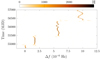 |
Fig. 1. Pulsar glitch analysis for PSR J0007+7303. The weighted H-test is calculated according to Eq. (2) using photons within the 170-day time window sliding over the entire data set with 17-day steps. For each window scans over f and ḟ were performed. The maximum value of H to ḟ for a given f is color-coded (see color scale at top). The vertical axis shows the time midpoint of each time window. The horizontal axis shows the offset in f. |
As can also be seen in Fig. 1, the maximum of the weighted H-test between glitches oscillates around a certain frequency. This effect is caused by the 3FGL sky-coordinates error reaching a few arcminutes due to the limited LAT angular resolution. As a result, the satellite’s motion relative to the source incorrectly taken into account leads to the Doppler modulation of the pulsations.
Figure 1 gives an example of the large Vela-type glitches of the size Δf/f ∼ 10−6, which are clearly visible to the naked eye in the H-test data despite the Doppler frequency shift. However, identification of small glitches of the size Δf/f ∼ 10−8 − 10−7 for gamma-ray pulsars may become a difficult problem, especially for fainter pulsars.
Another source of coherence loss is the poor background rejection if the pulsar is not very bright so that a large number of selected photons are not actually emitted by the pulsar. Figure 2 gives an example of such pulsars; PSR J2030+3641, which did not experience glitches during the considered period, and PSR J1422−6138, which experienced two glitches (Pletsch et al. 2013). In the computations we used coordinates from the Fermi-LAT 3FGL catalog; therefore, the Doppler shift of the frequency is present in the H-test data, which makes the glitches in the pulsar shown in Fig. 2b hardly distinguishable in the background of other frequency distortions.
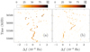 |
Fig. 2. Same as in Fig. 1, but for (a) PSR J2030+3641, without glitches during considered epochs, and (b) PSR J1422−6138, which experienced glitches at 55310 MJD and 55450 MJD. Computations were performed using the source coordinates from the Fermi-LAT 3FGL catalog. |
More accurate coordinates of the pulsar may be used in the analysis if they are known from other observations. If not, the loss of phase-coherence can be reduced by refining the sky-location of the source (Yu et al. 2013; Pletsch et al. 2013). However, it extends the parameter space of the scan to four dimensions (sky position, frequency, and spin-down rate). A more efficient selection of the photons has to be performed in the case that large background radiation causes frequency distortions in the H-test data. As a result, many samples corresponding to each attempt of the scan over coordinates and/or photon selection will be available for the analysis. Visual inspection of all of them is rather difficult. Therefore, a reliable criterion for automatic glitch search is required.
3. Convolutional neural network
Efficient identification of glitches, and of other peculiarities in the H-test data, may be obtained by using the machine learning approach. This provides an ability for the machine to “learn” specific patterns corresponding to the pulsar glitch directly from the data, without explicit definition. In the present paper we employ the convolutional neural network (CNN) (Fukushima 1980; Le Cun et al. 1989), a specialized kind of neural network for processing data with a grid-like structure. It is widely used in pattern recognition and image classification problems. In recent years CNNs have seen many applications in physics (Carleo et al. 2019) and astronomy (see, e.g., Kim & Brunner 2017; Petrillo et al. 2017; Hezaveh et al. 2017; Vernardos & Tsagkatakis 2019). In this section we show that CNNs are able to detect glitches in gamma-ray pulsars with high accuracy. This gives an opportunity for glitch identification in extensive searches dealing with the large amount of data when it cannot be done manually.
The CNN architecture used in this work is presented in Table 1. It was implemented in Python using Keras (Chollet 2015) library version 2.1.6 with the Tensorflow backend version 1.12.0. The network has two components: a feature extraction part and a classification part. The feature extraction part consists of convolution and polling layers with n and 2n filters, which detect specific patterns for both glitching and non-glitching pulsars; we assign the particular value of n below. The Dropout layer was used to prevent the network from overfitting. It works by randomly setting input units to 0 with a frequency of 0.5 at each step during the training stage. The classification part consist of two fully connected layers with 8n and one neuron. The REctified Linear Unit (ReLU) function is used for the inner and sigmoid for the output layer activations. The classification part outputs the probability that the input data corresponds to a glitching or non-glitching pulsar. A CNN output higher than 0.5 is interpreted as a glitch presence in the input sample.
Architecture of the convolutional neural network.
The weighted H-test dependence on frequency and time is used for glitch recognition. It is calculated in the way we discuss in Sect. 2. Before being fed to the CNN, the data is convolved with a Gaussian function according to the formula
 (3)
(3)
Searching for large glitches generally requires executing more steps in the scan over frequency. This considerably increases the size of the resulting H-test array. Thinning in this case will result in loss of high H-test values corresponding to some narrow frequency bandwidth. The convolution in Eq. (3) smooths small-scale details spreading the H-test values over the scales f ∼ δf. This allows the size of the array  to be reduced, keeping an average information. The convolution (3) can be calculated at any frequency within the range covered by the original data. In what follows we compute the convolution at 131 equidistant frequency values for every group of photons. As a result we obtain the array of size 131 × 131, which is fed to the CNN (see Table 1). This can be seen in Fig. 3, where the original data and the results of convolution are shown.
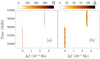 |
Fig. 3. Weighted H-test data calculated as discussed in Sect. 2 for (a) generated pulsar with glitch and (b) the same data after convolution with the Gaussian function (see Eq. (3)). |
The network contains a large number of trainable parameters, whose tuning requires a large amount of data. Since there are not very many known gamma-ray pulsars with glitches that can be employed to train the network, we generated a Monte Carlo set according to the following procedure. First, we randomly generated the pulsar frequency and spin-down rate within the ranges 1 Hz ≤ f ≤ 10 Hz and − 10−15 Hz s−1 ≤ ḟ ≤ −10−13 Hz s−1, respectively. Second, we assumed that the pulsar light curve is a Gaussian peak with the addition of a constant background level corresponding to the off-pulse emission. The width of a peak was generated randomly from 0.05 to 0.45 of the pulsar period 2π/f. The value of the constant background was generated from 0.1 to 0.6 of the peak height. For the pulsars with glitches we randomly generated the time after which the pulsar frequency and spin-down rate increase in the ranges 10−8 ≤ Δf/f ≤ 10−5 and 10−4 ≤ Δḟ/ḟ ≤ 10−3, respectively. Finally, we randomly generated 40 000 photons with unit weights according to this light curve with barycentric arrival times from 54682 MJD to 57084 MJD which corresponds to 6.5 years of Fermi-LAT observations.
The Monte Carlo set of 15 000 pulsars with glitches and 13 500 without glitches was generated. For each of the generated sources the weighed H-test data were calculated, as discussed in Sect. 2. The range of the scan over frequency was taken according to the glitch amplitude Δf and randomly for pulsars without glitches. The convolution was calculated according to Eq. (3). The results of applying the method to a typical generated pulsar with a glitch are illustrated in Fig. 3.
The data were split randomly into two subsets: 90% of the data for the training, 10% for the validation. In order to increase the amount of training data we employed an augmentation technique. We randomly cropped a region around a pre-glitch frequency value from the original array H(f, t) and by convolution with Gaussian function (3) we obtained  . The cross-entropy was used as the loss function assuming the target value of 1 for all samples of pulsars with glitches, and 0 otherwise. The network was trained during 150 epochs, while the overfitting was reduced by including a dropout layer and using L2 regularization of the weights in the convolutional layers.
The validation set was not involved in the training. It was used to provide an unbiased evaluation of the network performance. The accuracy of the network calculated on the validation data set during training is shown in Fig. 4. The parameter n, which parameterizes the number of independent filters (see Table 1), takes the value n = 16. The accuracy is defined as the ratio of the number of correct predictions to the total number of predictions. The figure shows that the network is successfully trained to recognize pulsars of both types. As can be seen, the accuracy does not improve much after the 50th epoch. Below we use the values from the 50th to the 150th epoch to estimate the average network accuracy (dashed line in Fig. 4).
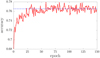 |
Fig. 4. Accuracy of the network with n = 16 over training epochs calculated on the validation set. The dashed line corresponds to an average accuracy from the 50th to the 150th epochs. |
The average accuracy defined above was used to tune the network architecture and the hyperparameters. In general, it includes the number of filters on the convolutional layers, the height and the width of the convolution windows, the size of the windows in the pooling layers, the number of neurons in the fully connected layer, and similar parameters. Tuning all of them is very challenging. For this reason we performed independent optimizations for parameter subsets.
First, we compared the performance of the networks with different number of filters in the convolutional layers parameterized by n, see Table 1. The average network accuracy on the validation data set as a function of n is shown in Fig. 5. The shadow region in the figure demonstrates the one-sigma deviation. As can be seen, the average accuracy initially grows with n and then reaches an approximately constant value for n > 10. Thus, the CNNs with n > 10 can be applied for glitch identification with approximately the same accuracy. Below we work with n = 16. In this case the number of free parameters of the CNN approximately equals the number of data samples in the training set.
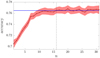 |
Fig. 5. Average network accuracy on the validation set depending on the number of filters in the convolutional layers parameterized by n (see Table 1). |
Second, we varied the number of neurons in the dense layer (see row 14 in the Table 1) for a fixed number of filters n = 16. We find that the average accuracy is approximately the same when the number of neurons is greater than 10.
Finally, we examined the average accuracy of the network with 5 × 5 convolution windows and with 3 × 3 pooling windows. Compared to the CNN in Table 1, it takes a smaller number of convolutional and pooling layers. For this reason it is less deep and contains fewer parameters. As a result, this CNN is about one percent less accurate than the original one.
Taking into account the above studies we settled on the CNN with the architecture presented in Table 1 with n = 16. It is accurate and not very complex. In order to test the accuracy of the CNN in more detail we generated an additional data set of 2500 pulsars without glitches and 2500 pulsars with glitches of the amplitude 10−10 Hz ≤ Δf ≤ 10−5 Hz. The network performance on the test data is presented in Fig. 6. The figure shows that the CNN demonstrates a high accuracy in the detection of large glitches. About 98% of pulsars with frequency change Δf ≳ 10−7 Hz are correctly identified. The false positive rate is about 2% over the whole frequency interval of the search. The example of pulsars with glitches correctly identified by the neural network is presented in Fig. 7.
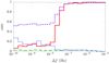 |
Fig. 6. Neural network efficiency of pulsar glitch detection. The true positive rate (red solid line) is the proportion of correctly identified pulsars with glitches among all pulsars with glitches of the amplitude Δf; the false positive rate (green dash-dotted line) is the proportion of erroneously identified pulsars with glitches among pulsars without glitches in the search for glitches of the amplitude Δf; accuracy (violet dashed line) is the proportion of correct predictions; and false discovery rate (blue dotted line) is the proportion of erroneously identified pulsars with glitches among all glitch identifications. |
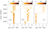 |
Fig. 7. Weighted H-test data calculated as discussed in Sect. 2, and convolved with Gaussian function (3) for three generated pulsars with glitches: (a) at 56183 MJD with Δf ≃ 4.6 × 10⁻⁸ Hz, (b) at 55045 MJD with Δf ≃ 4.2 × 10⁻⁷ Hz, and (c) at 56041 MJD with Δf ≃ 2.2 × 10⁻⁶ Hz. |
The fraction of pulsars with glitches identified correctly gradually decreases with decreasing amplitude of the frequency shift, reaching approximately 10% for Δf ≲ 10−8 Hz. We checked that an extension of the training set with pulsars with such small glitches does not improve the accuracy. This means that the method has reached the threshold of sensitivity, which corresponds to a resolution of the 170-day time window 1/Δt ≃ 7 × 10⁻⁸ Hz. The window size can be increased, but this does not seem to improve considerably the sensitivity to such small glitches.
The relative number of pulsars with glitches detected by the neural network below the sensitivity threshold was expected to be at the same level as the false positive rate. However, as can be seen in Fig. 6, this fraction is about 10%, which is much higher than 2%. The reason is in the non-negligible change in the spin-down rate generated in the range 10−4 ≤ Δḟ/ḟ ≤ 10−3. The weighted H-test calculated according to Eqs. (1) and (2) was maximized over the spin-down rate leaving dependence on t and f. However, some information about change in ḟ due to a glitch is likely to remain, and is “noticed” by the neural network. In order to test this hypothesis, we generated two sets of 100 pulsars each with the same glitch amplitude Δf = 10−10 Hz, but with different changes in the spin-down rate Δḟ = 10−20 Hz s−1 and Δḟ = 5 × 10⁻¹⁷ Hz s−1, respectively. The other parameters are fixed and are the same in both sets. The result of applying the neural network to these two sets confirmed the hypothesis: In the set with Δḟ = 10−20 Hz s−1 two pulsars were correctly identified, while in another set the CNN identified 11 samples as pulsars with glitches.
4. Discussion
In this paper we showed that the convolutional neural network applied to the weighted H-test data can be used to detect glitches in the gamma-ray pulsars in an automatic regime. The neural network demonstrates a very high accuracy on the generated sets and recognizes pulsars with glitches down to very small amplitudes Δf ∼ 10−8 Hz. It opens up a new possibility to exploit this method in extensive searches dealing with a large volume of data.
In order to verify the network’s ability to recognize glitches in the real data, we applied it to several gamma-ray pulsars from the Fermi-LAT 3FGL catalog. The neural network correctly identified pulsars with glitches known previously, including those presented in Figs. 1 and 2. We postpone an extensive search of new glitches with the adjustment of coordinates to future works.
It is worth noting that in this paper we did not apply the neural network to the large volume of real data, which can turn out to be more complicated for glitch recognition. In this case the following improvements of the method are possible. First of all, the scan over source coordinates will be able to recover phase-coherence, and consequently will increase the sensitivity of the method. Second, some features of the real data that confuse the network can be implemented in the Monte Carlo set. This will help to regain the accuracy achieved with the training set.
Acknowledgments
We thank the anonymous referee, O.E. Kalashev, G.I. Rubtsov, and Y.V. Zhezher for helpful comments and discussions. The work is supported by the Russian Science Foundation grant 17-72-20291. The numerical part of the work is performed at the cluster of the Theoretical Division of INR RAS.
References
- Abdo, A. A., Ackermann, M., Ajello, M., et al. 2009, Science, 325, 840 [Google Scholar]
- Abdo, A. A., Ajello, M., Allafort, A., et al. 2013, ApJS, 208, 17 [Google Scholar]
- Acero, F., Ackermann, M., & Ajello, M. 2015, ApJS, 218, 41 [Google Scholar]
- Atwood, W. B., Abdo, A. A., Ackermann, M., et al. 2009, ApJ, 697, 1071 [CrossRef] [Google Scholar]
- Ball, N. M., & Brunner, R. J. 2010, Int. J. Mod. Phys. D, 19, 1049 [Google Scholar]
- Baron, D. 2019, ArXiv e-prints [arXiv:1904.07248] [Google Scholar]
- Bertsch, D. L., Brazier, K. T. S., Fichtel, C. E., et al. 1992, Nature, 357, 306 [NASA ADS] [CrossRef] [Google Scholar]
- Carleo, G., Cirac, I., Cranmer, K., et al. 2019, Rev. Mod. Phys., 91, 045002 [NASA ADS] [CrossRef] [Google Scholar]
- Chollet, F. 2015, https://github.com/fchollet/keras [Google Scholar]
- Clark, C. J., Pletsch, H. J., Wu, J., et al. 2015, ApJ, 809, L2 [NASA ADS] [CrossRef] [Google Scholar]
- Clark, C. J., Wu, J., & Pletsch, H. J. 2017, ApJ, 834, 106 [NASA ADS] [CrossRef] [Google Scholar]
- Cordes, J. M., Downs, G. S., & Krause-Polstorff, J. 1988, ApJ, 330, 847 [NASA ADS] [CrossRef] [Google Scholar]
- de Jager, O. C., & Busching, I. 2010, A&A, 517, L9 [NASA ADS] [CrossRef] [EDP Sciences] [Google Scholar]
- de Jager, O. C., Raubenheimer, B. C., & Swanepoel, J. W. H. 1989, A&A, 221, 180 [NASA ADS] [Google Scholar]
- Eatough, R. P., & Molkenthin, N., & Kramer, M., 2010, MNRAS, 407, 2443 [NASA ADS] [CrossRef] [Google Scholar]
- Espinoza, C. M., Lyne, A. G., Stappers, B. W., & Kramer, M. 2011, MNRAS, 414, 1679 [NASA ADS] [CrossRef] [Google Scholar]
- Espinoza, C. M., Antonopoulou, D., Stappers, B. W., Watts, A., & Lyne, A. G. 2014, MNRAS, 440, 2755 [NASA ADS] [CrossRef] [Google Scholar]
- Fukushima, K. 1980, Biol. Cybern., 36, 193 [CrossRef] [PubMed] [Google Scholar]
- Halpern, J. P., & Holt, S. S. 1992, Nature, 357, 222 [NASA ADS] [CrossRef] [Google Scholar]
- Haskell, B., & Melatos, A. 2015, Int. J. Mod. Phys. D, 24, 1530008 [NASA ADS] [CrossRef] [Google Scholar]
- Hezaveh, Y. D., Perreault Levasseur, L., & Marshall, P. J. 2017, Nature, 548, 555 [Google Scholar]
- Kim, E. J., & Brunner, R. J. 2017, MNRAS, 464, 4463 [Google Scholar]
- Le Cun, Y., Guyon, I., Jackel, L. D., et al. 1989, Commun. Mag., 27, 41 [CrossRef] [Google Scholar]
- Li, J., Torres, D. F., de Ona Wilhelmi, E., Rea, N., & Martin, J. 2016, ApJ, 831, 19 [NASA ADS] [CrossRef] [Google Scholar]
- Lyne, A. G., Shemar, S. L., & Graham-Smith, F. 2000, MNRAS, 315, 534 [NASA ADS] [CrossRef] [Google Scholar]
- Lyne, A. G., Jordan, C. A., Graham-Smith, F., et al. 2015, MNRAS, 446, 857 [NASA ADS] [CrossRef] [Google Scholar]
- McKee, J. W., Janssen, G. H., Stappers, B. W., et al. 2016, MNRAS, 461, 2809 [NASA ADS] [CrossRef] [Google Scholar]
- McKenna, J., & Lyne, A. G. 1990, Nature, 343, 349 [NASA ADS] [CrossRef] [Google Scholar]
- Packard, R. E. 1972, Phys. Rev. Lett., 28, 1080 [NASA ADS] [CrossRef] [Google Scholar]
- Palfreyman, J., Dickey, J. M., Hotan, A., Ellingsen, S., & van Straten, W. 2018, Nature, 556, 219 [NASA ADS] [CrossRef] [Google Scholar]
- Petrillo, C. E., Tortora, C., Chatterjee, S., et al. 2017, MNRAS, 472, 1129 [Google Scholar]
- Pletsch, H. J., Guillemot, L., Allen, B., et al. 2012, ApJ, 755, L20 [NASA ADS] [CrossRef] [Google Scholar]
- Pletsch, H. J., Guillemot, L., Allen, B., et al. 2013, ApJ, 779, L11 [NASA ADS] [CrossRef] [Google Scholar]
- Radhakrishnan, V., & Manchester, R. N. 1969, Nature, 222, 228 [NASA ADS] [CrossRef] [Google Scholar]
- Reichley, P. E., & Downs, G. S. 1969, Nature, 222, 229 [NASA ADS] [CrossRef] [Google Scholar]
- Ruderman, M. 1969, Nature, 223, 597 [NASA ADS] [CrossRef] [Google Scholar]
- Saz Parkinson, P. M., Dormody, M., Ziegler, M., et al. 2010, ApJ, 725, 571 [Google Scholar]
- Shannon, R. M., Lentati, L. T., Kerr, M., et al. 2016, MNRAS, 459, 3104 [NASA ADS] [CrossRef] [Google Scholar]
- Sokolova, E., & Rubtsov, G. 2016, ApJ, 833, 271 [NASA ADS] [CrossRef] [Google Scholar]
- Vernardos, G., & Tsagkatakis, G. 2019, MNRAS, 486, 1944 [NASA ADS] [CrossRef] [Google Scholar]
- Vivekanand, M. 2017, ArXiv e-prints [arXiv:1710.05293] [Google Scholar]
- Yu, M., Manchester, R. N., Hobbs, G., et al. 2013, MNRAS, 429, 688 [NASA ADS] [CrossRef] [Google Scholar]
All Tables
All Figures
|
Fig. 1. Pulsar glitch analysis for PSR J0007+7303. The weighted H-test is calculated according to Eq. (2) using photons within the 170-day time window sliding over the entire data set with 17-day steps. For each window scans over f and ḟ were performed. The maximum value of H to ḟ for a given f is color-coded (see color scale at top). The vertical axis shows the time midpoint of each time window. The horizontal axis shows the offset in f. |
| In the text | |
|
Fig. 2. Same as in Fig. 1, but for (a) PSR J2030+3641, without glitches during considered epochs, and (b) PSR J1422−6138, which experienced glitches at 55310 MJD and 55450 MJD. Computations were performed using the source coordinates from the Fermi-LAT 3FGL catalog. |
| In the text | |
|
Fig. 3. Weighted H-test data calculated as discussed in Sect. 2 for (a) generated pulsar with glitch and (b) the same data after convolution with the Gaussian function (see Eq. (3)). |
| In the text | |
|
Fig. 4. Accuracy of the network with n = 16 over training epochs calculated on the validation set. The dashed line corresponds to an average accuracy from the 50th to the 150th epochs. |
| In the text | |
|
Fig. 5. Average network accuracy on the validation set depending on the number of filters in the convolutional layers parameterized by n (see Table 1). |
| In the text | |
|
Fig. 6. Neural network efficiency of pulsar glitch detection. The true positive rate (red solid line) is the proportion of correctly identified pulsars with glitches among all pulsars with glitches of the amplitude Δf; the false positive rate (green dash-dotted line) is the proportion of erroneously identified pulsars with glitches among pulsars without glitches in the search for glitches of the amplitude Δf; accuracy (violet dashed line) is the proportion of correct predictions; and false discovery rate (blue dotted line) is the proportion of erroneously identified pulsars with glitches among all glitch identifications. |
| In the text | |
|
Fig. 7. Weighted H-test data calculated as discussed in Sect. 2, and convolved with Gaussian function (3) for three generated pulsars with glitches: (a) at 56183 MJD with Δf ≃ 4.6 × 10⁻⁸ Hz, (b) at 55045 MJD with Δf ≃ 4.2 × 10⁻⁷ Hz, and (c) at 56041 MJD with Δf ≃ 2.2 × 10⁻⁶ Hz. |
| In the text | |
Current usage metrics show cumulative count of Article Views (full-text article views including HTML views, PDF and ePub downloads, according to the available data) and Abstracts Views on Vision4Press platform.
Data correspond to usage on the plateform after 2015. The current usage metrics is available 48-96 hours after online publication and is updated daily on week days.
Initial download of the metrics may take a while.