| Issue |
A&A
Volume 659, March 2022
|
|
|---|---|---|
| Article Number | A184 | |
| Number of page(s) | 6 | |
| Section | Extragalactic astronomy | |
| DOI | https://doi.org/10.1051/0004-6361/202142051 | |
| Published online | 24 March 2022 | |
Can the one-zone hadronuclear model explain the hard-TeV spectrum of BL Lac objects?
1
Department of Physics, Zhejiang Normal University, Jinhua 321004, PR China
e-mail: ruixue@zjnu.edu.cn
2
School of Physics, Sun Yat-sen University, Guangzhou, GuangDong, PR China
3
College of Physics and Electronic Engineering, Qilu Normal University, Jinan 250200, PR China
4
Astrophysical Big Bang Laboratory (ABBL), RIKEN, Saitama 351-0198, Japan
5
Interdisciplinary Theoretical & Mathematical Science Program (iTHEMS), RIKEN, Saitama 351-0198, Japan
6
Yunnan Observatories, Chinese Academy of Sciences, Kunming 650011, PR China
7
Key Laboratory for the Structure and Evolution of Celestial Objects, Chinese Academy of Sciences, Kunming 650011, PR China
Received:
19
August
2021
Accepted:
30
January
2022
Context. The intrinsic TeV emission of some BL Lacs is characterized by a hard spectrum (the hard-TeV spectrum) after correcting for the extragalactic background light. The hard-TeV spectra pose a challenge to conventional one-zone models, including the leptonic model, the photohadronic model, the proton synchrotron model, and others.
Aims. In this work, we aim to investigate whether or not the one-zone hadronuclear (pp) model can be used to interpret the hard-TeV spectra of BL Lacs without introducing extreme parameters.
Methods. We provide analytical calculations that can be used to study whether or not there is a parameter space, and whether or not the charge neutrality condition of the jet can be satisfied when interpreting the hard-TeV spectra of BL Lacs without introducing a super-Eddington jet power.
Results. We find that in a sample of hard-TeV BL Lacs previously collected, only the hard-TeV spectrum of 1ES 0229+200 can be explained by γ-rays from π0 decay produced in the pp interactions, but at the cost of setting a small radius of the radiation region than the Schwarzschild radius of the central black hole. Combining our findings with those of previous studies of other one-zone models, we suggest that the hard-TeV spectra of BL Lacs cannot be explained by a one-zone model without introducing extreme parameters, and should originate from the multiple radiation regions.
Key words: galaxies: active / galaxies: jets / radiation mechanisms: non-thermal
© ESO 2022
1. Introduction
Blazars are a class of active galactic nuclei (AGNs) with their relativistic jets pointing to the observer (Urry & Padovani 1995). Multi-wavelength observations, when combined, show that the spectral energy distributions (SEDs) of blazars usually exhibit two characteristic bumps. It is generally accepted that the low-energy bump originates from the synchrotron radiation of primary relativistic electrons in the jet, while the origin of the high-energy bump is still debated. In leptonic models, the high-energy bump is explained by inverse Compton (IC) radiation from relativistic electrons that up-scatter soft photons emitted by the same population of electrons (synchrotron-self Compton, SSC; Marscher & Gear 1985), or soft photons from external photon fields (external Compton, EC) such as the accretion disk (Dermer & Schlickeiser 1993), the broad-line region (BLR, Sikora et al. 1994), or the dusty torus (DT, Błażejowski et al. 2000). In hadronic models, the high-energy bump is supposed to be originated from proton synchrotron radiation (Aharonian 2000), emission from secondary particles generated in photohadronic processes (pγ), including photopion and Bethe-Heitler pair production processes (Sahu et al. 2019) and the internal γγ pair production, or cascade emission generated in the intergalactic space through pγ interactions by ultra-high energy cosmic rays (UHECRs) with energies up to 1019 − 20 eV beamed by the blazar jet (e.g., Essey et al. 2011).
The extragalactic TeV background is dominated by emission from blazars (Ackermann et al. 2016), most of which are BL Lacertae objects1 (BL Lacs; Urry & Padovani 1995). After correcting for the extragalactic background light (EBL) absorption, the obtained intrinsic TeV emission of some BL Lacs often shows a hard spectrum, that is, the photon index ΓTeV < 2 (hereafter the hard-TeV spectrum). However, some intrinsic TeV spectra are too hard to be interpreted by conventional radiation models. In the modeling of the radiation from blazars, it is usually assumed that all the non-thermal emission of the jet comes from a compact spherical region named the blob. Such a model is also known as the one-zone model, where the one-zone leptonic model is the most commonly used (e.g., Ghisellini et al. 2014; Tan et al. 2020; Deng et al. 2021). However, as the Klein-Nishina (KN) effect softens the IC emission in the TeV band naturally, the one-zone leptonic model cannot reproduce the hard-TeV spectrum unless setting an extremely high Doppler factor (e.g., Aleksić et al. 2012) –which is in conflict with radio observations (Hovatta et al. 2009)– and/or introducing a very high value of the minimum electron Lorentz factor (e.g., Katarzyński et al. 2006). In the modeling of blazars, the one-zone pγ model is also widely applied. To explain the hard-TeV spectrum, an extremely high proton power is required because the pγ interaction is very inefficient. Based on the fact that the interaction efficiency of the photopion process in the high-energy limit is about 1000 times smaller than the bump of γγ opacity, Xue et al. (2019a) prove that the required minimum jet powers of a sample of hard-TeV BL Lacs exceed the corresponding Eddington luminosities of the supermassive black holes (SMBHs). For the emitting region with a strong magnetic field (10–100 G), the one-zone proton synchrotron model is also widely applied to explain the high-energy bump (Böttcher et al. 2013). However, the super-Eddington jet power is also needed (Zdziarski & Bottcher 2015), except in a few cases such as the fast variabilities (tν ≤ 103s; Petropoulou & Dermer 2016) and very hard injection functions (α ≤ 1.5; Cerruti et al. 2015). In addition, some studies suggest that the magnetic field in the inner jet of blazars is typically lower than 10 G (O’Sullivan & Gabuzda 2009; Meyer et al. 2014). If the hard-TeV spectrum is still explained by the proton synchrotron emission in a magnetic field ≲10 G, the maximum proton energy larger than that obtained from the Hillas condition (EHillas; Hillas 1984) has to be assumed. The cascade emission from the UHECR can explain the hard-TeV spectrum as well, but may also need extremely high maximum proton energies higher than EHillas (Takami et al. 2016, cf., Das et al. 2020). Also, the hard-TeV spectra of some BL Lacs show variabilities (e.g., Acciari et al. 2010), which disfavor the cascade emission from UHECRs (e.g., Prosekin et al. 2012). Overall, the hard-TeV spectra pose a challenge to conventional one-zone models.
Of the various one-zone models introduced above, the one-zone hadronuclear (pp) model has not been studied comprehensively. In studies investigating the radiation mechanisms of the jets of blazars, the pp interaction is normally neglected, because the particle density in the jet is considered insuffient (Atoyan & Dermer 2003). Several associations between high-energy neutrinos and blazars have recently been discovered (e.g., IceCube Collaboration 2018). However, these events are difficult to explain using the conventional one-zone pγ model (e.g., Xue et al. 2019b, 2021), and therefore several innovative pp models are proposed (e.g., Sahakyan 2018; Banik & Bhadra 2019; Liu et al. 2019; Wang & Xue 2022). Also, Xue et al. (2019a) suggest that the one-zone pp model may provide a possible solution to reproducing the hard TeV spectrum with a sub-Eddington jet power, as the efficiency of pp interactions is not related to the opacity of γγ absorption. Therefore, further comprehensive consideration of the pp interaction in the one-zone model is necessary in order to understand the origin of the hard-TeV spectra of BL Lacs.
In this paper, we analytically study whether the hard-TeV spectra of BL Lacs can be explained without violating basic observations and theories in one-zone pp models. In Sect. 2, we present analytical methods to find the parameter space, and then study if the charge neutrality condition can be satisfied in the framework of one-zone pp models. We present the discussion and the conclusion in Sect. 3. Throughout the paper, the ΛCDM cosmological parameters H0 = 70 km s−1 Mpc−1, Ωm = 0.3, and ΩΛ = 0.7 are adopted.
2. Analytical calculations
For blazar jets, the pp process is usually considered in interactions between the jet and its surrounding materials, such as dense clouds in the BLR, and red giant stars captured from the host galaxy (e.g., Bosch-Ramon et al. 2012). However, it is unclear whether or not the jet inside has sufficient cold protons. Here, we propose analytical methods to study whether or not the hard-TeV spectra of BL Lacs can be explained by the one-zone pp model, which, considering the pp interactions, occur in the jet without introducing extreme parameters. We also study whether or not the charge neutrality condition of the jet can be satisfied, although this commonly assumed condition (Ghisellini et al. 2014) remains a matter of debate (Chen & Zhang 2021).
It should be noted that the jet composition is currently uncertain. In addition to electrons and protons, there may be a certain number of other charged particles in the jet, such as positrons (e.g., Madejski et al. 2016). In a jet that satisfies the charge neutrality condition, the contribution from pp interactions becomes weaker if there is a large number of positrons, thus making the model parameters more extreme. In this work, our main purpose is to study the maximum parameter space under the one-zone pp model, and therefore we boldly assume that the charged particles in the jet consist only of electrons and protons, both relativistic and non-relativistic.
The following analytical calculation of searching the parameter space is under the framework of the conventional one-zone model. We assume that all of the nonthermal radiation of the observed jet comes from a single spherical region (hereafter referred to as the blob) composed of a plasma of charged particles in a uniformly entangled magnetic field B with radius R and moving with the bulk Lorentz factor  , where βc is the speed of the blob, at a viewing angle with respect to the line of sight of the observer. For the relativistic jet close to the line of sight in blazars with a viewing angle of θ ≲ 1/Γ, we have the Doppler factor δ ≈ Γ. In this section, the parameters with superscript “obs” are measured in the frame of the observer, those with superscript “AGN” are measured in the AGN frame, whereas the parameters without the superscript are measured in the comoving frame, unless specified otherwise.
2.1. Methods
For the hard-TeV spectrum, as the SSC emission cannot explain it because of the KN effect, we suppose that it can be interpreted by the γ-ray from π0 decay produced in the pp interactions. The proton injection luminosity can be calculated as
where mp is the rest mass of a proton, c is the speed of light, and
represents the average proton Lorentz factor, where  is the injection rate of proton energy distribution, ṅ0,p is the normalization in units of cm−3 s−1, αp is the proton spectral index, γp is the proton Lorentz factor, γp, min is the minimum proton Lorentz factor, and γp, max is the maximum proton Lorentz factor, and
  is the energy-integrated number density of injected relativistic protons. This pp explanation has two main constraints. The first is that the generated γ-ray luminosity from π0 decay exceeds the observed TeV luminosity, as the intrinsic hard-TeV spectrum may not be truncated at the maximum energy currently observed, but will extend to higher energy, i.e.,
where
is the pp interaction efficiency, the factor 1/3 is the branching ratio into π0, σpp ≈ 6 × 10⁻²⁶ cm2 is the cross section for the pp interactions, nH is the number density of cold protons in the jet, and Kpp ≈ 0.5 is the inelasticity coefficient (Kelner et al. 2006). The other constraint is that the total jet power that is dominated by the power of relativistic and nonrelativistic protons cannot exceed the Eddington luminosity of the SMBH, otherwise the growth of the SMBH would be too quick (Antognini et al. 2012). Therefore, we have
where  is the power of the injected relativistic protons in the AGN frame,
is the Eddington luminosity of the SMBH, σT is the Thomson scattering cross-section, RS = 2GMBH/c2 is the Schwarzschild radius of the SMBH, MBH is the SMBH mass,
is the kinetic power in cold protons. In order to find the maximum parameter space, we assume that the π0 decay generates the required minimum γ-ray luminosity, i.e.,  . Substituting
  , Eqs. (4), (6), and (7) into Eq. (5), we then have
If  is taken as an independent variable, Eq. (8) becomes a quadratic formula. Here, the quadratic formula can take the minimum value when
  is LEdd/2. Substituting
  into Eq. (8), the maximum parameter space of R can then be obtained through
when the SMBH mass and TeV luminosity are measured.
In the above analytical calculations, by fixing the γ-ray luminosity from π0 decay to the required minimum value, and keeping the total jet power at or below the Eddington luminosity of the SMBH, the parameter space of R is well constrained. Similarly, the maximum parameter space of R can also be obtained by fixing the total jet power to the Eddington luminosity of the SMBH, which is the maximum value that can be set, and making the γ-ray luminosity from π0 decay larger than the observed TeV luminosity. Here, the power of the injected relativistic protons is considered as a fraction χp of the total jet power, which is
As the power of the relativistic and nonrelativistic electrons is normally negligible compared to that of relativistic and nonrelativistic protons, according to Eq. (7) and Eq. (10), nH can be estimated as
The γ-ray luminosity from π0 decay produced in the pp interactions can be given by
Combining with Eqs. (4), (10)–(12), if the hard-TeV spectrum can be interpreted by the γ-ray from π0 decay produced in the pp interactions, we can get
In order to get the maximum parameter space, it is necessary to set χp = 0.5, which is consistent with the result obtained below Eq. (8). If further substituting Eq. (6) into Eqs. (13), (9) can also be derived.
Xue et al. (2019a) collected a sample of hard-TeV BL Lacs with measured TeV luminosities and SMBH masses. Their corresponding maximum R obtained by Eq. (9) are shown in Table 1. It can be seen that the derived maximum R is relatively small, and is comparable to or even smaller than the Schwarzschild radius of the SMBH RS. However, in such a compact blob, TeV photons are likely to be absorbed due to the internal γγ absorption. As the spectral shape of soft photons is fixed by observational data points, that is, the low-energy component, the internal γγ absorption optical depth is only related to R and δ, i.e., τγγ ∝ R−1δ−4. Xue et al. (2019a) give the value of R and δ when τγγ of the maximum energy of the hard-TeV spectrum is equal to unity. Therefore, in order to prevent the hard-TeV spectrum being absorbed, a larger δ must be introduced, because the maximum R shown in Table 1 is already much smaller than that given by Xue et al. (2019a). If the maximum δ that can be set is 30, as indicated by observations (Hovatta et al. 2009), only 1ES 0229+200 has the parameter space needed to interpret the hard-TeV spectrum with the one-zone pp model.
Sample of hard-TeV BL Lacs collected by Xue et al. (2019a).
2.2. Charge neutrality condition of the jet
Recently, Banik & Bhadra (2019) suggested that when considering the charge neutrality condition of the blazar jet, there is sufficient cold protons, making the pp interaction efficient and explaining the observed TeV γ-ray and neutrino emission from the blazar TXS 0506+056. However, if the kinetic power of cold protons is taken into account, a super-Eddington jet power is still needed, because the blob radius introduced in their modeling is about a hundred times larger than that obtained by our analytical methods. In the following, we investigate whether or not the charge neutrality condition of the jet can be satisfied when interpreting the hard-TeV spectra without introducing a super-Eddington jet power.
Due to the lack of strong emission from external photon fields in TeV BL Lacs, it is generally accepted that the emission below ∼100 GeV originates from the synchrotron and SSC emission from primary relativistic electrons. The electron injection luminosity can be calculated as
where me is the rest mass of an electron, and
is the average electron Lorentz factor, where  is the injection rate of electron energy distribution (EED), ṅ0,e is the normalization in units of cm−3 s−1, αe is the electron spectral index, γe is the electron Lorentz factor, γe, min is the minimum electron Lorentz factor, and γe, max is the maximum electron Lorentz factor, and
  is the energy-integrated number density of injected relativistic electrons. Taking into account cold electrons that are not accelerated or cooled, the total number density of electrons in the jet ne, tot can be approximated as

where χe represents the ratio of ne, tot to ne and

is the number density of relativistic electrons, where tdyn = R/c is the dynamical timescale of the blob2.
As the cooling of relativistic protons in the jet is inefficient, the number density of relativistic protons can be approximated as

Under the charge neutrality condition, combining Eqs. (16) and (18), we get the number density of cold protons in the jet through
Substituting Eqs. (1) and (14) into Eq. (19), we have
Further substituting Eq. (20) into Eqs. (3) and 5, we obtain
![$$ \begin{aligned}&\frac{\langle \gamma _{\rm e} \rangle }{L_{\rm e,inj}}\frac{m_{\rm e}}{m_{\rm p}}\left(4\frac{\sigma _{\rm T}}{\sigma _{\rm pp}}\frac{R}{R_{\rm S}}\frac{L_{\rm TeV}^\mathrm{obs}}{\chi _{\rm p}\delta ^2}+\frac{L_{\rm p,inj}}{\langle \gamma _{\rm p} \rangle }\right) \le \chi _{\rm e} \nonumber \\&\quad \le \langle \gamma _{\rm e} \rangle \frac{L_{\rm p,inj}}{L_{\rm e,inj}}\frac{m_{\rm e}}{m_{\rm p}}\left[\frac{4(1-\chi _p)}{3\chi _p} + \frac{1}{\langle \gamma _{\rm p} \rangle }\right]. \end{aligned} $$](/articles/aa/full_html/2022/03/aa42051-21/aa42051-21-eq33.gif)
With the above inequalities, the range of χe satisfying the charge neutrality condition can be obtained. It is difficult to find a concise expression of the above inequalities because the number density of relativistic electrons is greatly affected by the shape and energy range of EED, and γe, min and γe, max are poorly constrained in one-zone models. In any case, the above inequalities suggest that, even though R is small, χe still has a parameter space to satisfy the charge neutrality condition. Here, we take TXS 0506+056 as an example. If we set R as its maximum value given in Table 1, and values of other parameters as those provided by Banik & Bhadra (2019) 3, the range of χe as a function of χp obtained by Eq. (21) is shown by the intersection area of black (upper limit) and red (lower limit) solid curves in Fig. 1. The vertical line in Fig. 1 marks the position of χp = 0.5. We find that when χp = 0.5, χe has the largest range of values, which is consistent with the result obtained in Sect. 2.1. In addition, the comparison results of adjusting some other parameters are also shown in Fig. 1. It can be seen that adjusting the electron injection luminosity (dotted curves) and the Doppler factor (dashed-dotted curves) will change the parameter space of χe but the size of the intersection area of the upper and lower limits remains the same. Also, when setting a larger blob radius RB\AMP B = 2.2 × 1016 cm, such as that used in Banik & Bhadra (2019), the lower limit represented by the red dashed curve is much higher than the upper limit represented by the black solid curve (as adjusting blob radius does not affect the upper limit, the black dashed curve is overlapped by the black solid curve), which suggests that a highly super-Eddington jet power has to be introduced.
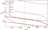 |
Fig. 1. Comparison of χe as a function of χp derived by Eq. (21) with different parameters. For all the line styles, the black and red curves represent the upper and lower limits, respectively. The solid curves are obtained when setting R as the maximum value given in Table 1 and values of other parameters as those provided by Banik & Bhadra (2019). Based on this, the dotted curves show the upper and lower limits when setting the electron injection luminosity to |

3. Discussion and conclusion
In this work, we investigated whether or not one-zone pp models are able to explain the hard-TeV spectra of BL Lacs. With analytical calculations, we find that an extremely compact radiation region has to be assumed if the hard-TeV spectrum is interpreted as γ rays produced from π0 decay in the pp interaction. However, if considering the internal γγ opacity at the TeV band to be less than unity and a Doppler factor of smaller than 30, only the hard-TeV spectra of 1ES 0229+200 can be explained. However, the allowable maximum radius of the blob under the constraints of Eq. (9) is very small, and is comparable to the Schwarzschild radius of the SMBH. This compact blob might be a relativistically moving plasmoid generated in the magnetic reconnection of the jet inside (Aharonian et al. 2017), implying a fast minute-scale variability, which is observed in the TeV band of radio galaxies (e.g., Aleksić et al. 2014) and blazars (e.g., Albert et al. 2007). Nevertheless, no evidence of fast variability in the TeV band of 1ES 0229+200 is found, and therefore the injection of relativistic protons in such a compact blob must be continuous. On the other hand, it can be seen from Eq. (9) that for AGNs with low TeV luminosity, such as radio galaxies, the effective pp processes can occur in a large-scale region (e.g., lobes) far from the SMBH, which could be the possible origin of the TeV spectrum (e.g., Sun et al. 2016).
In addition to conventional radiation models of blazars, another possible solution invoked is the hypothetical conversion between axion-like particles (ALPs) and propagating γ-ray photons in an external magnetic field, which has been widely investigated as an explanation of the TeV emission of blazars (e.g., Sánchez-Conde et al. 2009). The conversion could enable propagating TeV-photons to avoid γγ absorption, leading to the very hard-TeV spectrum observed (e.g., Long et al. 2020, 2021). If it takes place in the blob of the inner jet with a strong magnetic field, the effective conversion occurs on the GeV-photons, and the ALPs converted from the source photons cannot reconvert into photons in the lower Galactic magnetic field (Tavecchio et al. 2015). As a result, a substantial fraction of GeV photons would be lost, and this may also lead to the excessive Eddington luminosity of the SMBH. Conversely, if this conversion were to occur in the large-scale jet (also the TeV emission region) with a weaker magnetic field, this problem would be avoided.
Indeed, the different variability patterns between TeV emission and other wavelength emission discovered for some hard-TeV BL Lacs may favor a multi-zone origin of the hard-TeV spectra. For example, a TeV flare of the hard-TeV BL Lac 1ES 1215+303 was found by MAGIC in 2011, while no variability was found in the GeV band at the same time (Aleksić et al. 2012). Also, no fast variability in the TeV band is found for many hard-TeV BL Lacs, while other wavelength emissions are highly variable (e.g., 1ES 0229+200; Aliu et al. 2014).
In summary, we investigate whether or not the hard-TeV spectra of BL Lacs can be explained with the one-zone pp model, which completes the application of the one-zone model to studying the hard-TeV spectra of BL Lacs. Unfortunately, 1ES 0229+200 can only be explained if we introduce a very small blob radius comparable to the Schwarzschild radius of a SMBH. Therefore, combined with previous studies that applied other one-zone models, we suggest that no one-zone model can explain the hard-TeV spectra of BL Lacs in general. Such spectra are likely to originate from multiple emitting regions (e.g., Yan et al. 2012). Furthermore, the region generating the emission below ∼100 GeV and the region producing the hard-TeV spectrum should be decoupled (Wang et al. 2022). Both leptonic and hadronic processes could possibly explain the hard-TeV spectrum of BL Lacs.
This relation comes from the fact that the radiative cooling of most electrons is in the slow cooling regime for BL Lacs. Although the cooling of high-energy electrons might be in the fast cooling regime, the result would not be significantly different because the number density of relativistic electrons ne, rel is dominated by the low-energy electrons that dissipated in the slow cooling regime.
Acknowledgments
We thank the anonymous referee for insightful comments and constructive suggestions. This work was supported by JSPS KAKENHI Grant JP19H00693. This work was supported in part by a RIKEN pioneering project “Evolution of Matter in the Universe (r-EMU)”.
References
- Acciari, V. A., Aliu, E., Beilicke, M., et al. 2010, ApJ, 709, L163 [NASA ADS] [CrossRef] [Google Scholar]
- Ackermann, M., Ajello, M., Albert, A., et al. 2016, Phys. Rev. Lett., 116, 151105 [NASA ADS] [CrossRef] [Google Scholar]
- Aharonian, F. A. 2000, New Astron., 5, 377 [NASA ADS] [CrossRef] [Google Scholar]
- Aharonian, F. A., Barkov, M. V., & Khangulyan, D. 2017, ApJ, 841, 61 [NASA ADS] [CrossRef] [Google Scholar]
- Albert, J., Aliu, E., Anderhub, H., et al. 2007, ApJ, 669, 862 [Google Scholar]
- Aleksić, J., Alvarez, E. A., Antonelli, L. A., et al. 2012, A&A, 544, A142 [NASA ADS] [CrossRef] [EDP Sciences] [Google Scholar]
- Aleksić, J., Ansoldi, S., Antonelli, L. A., et al. 2014, Science, 346, 1080 [Google Scholar]
- Aliu, E., Archambault, S., Arlen, T., et al. 2014, ApJ, 782, 13 [NASA ADS] [CrossRef] [Google Scholar]
- Antognini, J., Bird, J., & Martini, P. 2012, ApJ, 756, 116 [NASA ADS] [CrossRef] [Google Scholar]
- Atoyan, A. M., & Dermer, C. D. 2003, ApJ, 586, 79 [Google Scholar]
- Banik, P., & Bhadra, A. 2019, Phys. Rev. D, 99, 103006 [NASA ADS] [CrossRef] [Google Scholar]
- Bosch-Ramon, V., Perucho, M., & Barkov, M. V. 2012, A&A, 539, A69 [NASA ADS] [CrossRef] [EDP Sciences] [Google Scholar]
- Böttcher, M., Reimer, A., Sweeney, K., et al. 2013, ApJ, 768, 54 [NASA ADS] [CrossRef] [Google Scholar]
- Błażejowski, M., Sikora, M., Moderski, R., et al. 2000, ApJ, 545, 107 [CrossRef] [Google Scholar]
- Cerruti, M., Zech, A., Boisson, C., et al. 2015, MNRAS, 448, 910 [NASA ADS] [CrossRef] [Google Scholar]
- Chen, L., & Zhang, B. 2021, ApJ, 906, 105 [NASA ADS] [CrossRef] [Google Scholar]
- Das, S., Gupta, N., & Razzaque, S. 2020, ApJ, 889, 149 [NASA ADS] [CrossRef] [Google Scholar]
- Deng, X.-J., Xue, R., Wang, Z.-R., et al. 2021, MNRAS, 506, 5764 [NASA ADS] [CrossRef] [Google Scholar]
- Dermer, C. D., & Schlickeiser, R. 1993, ApJ, 416, 458 [Google Scholar]
- Essey, W., Ando, S., & Kusenko, A. 2011, Astropart. Phys., 35, 135 [NASA ADS] [CrossRef] [Google Scholar]
- Ghisellini, G., Tavecchio, F., Maraschi, L., et al. 2014, Nature, 515, 376 [Google Scholar]
- Gupta, S. P., Pandey, U. S., Singh, K., et al. 2012, New Astron., 17, 8 [NASA ADS] [CrossRef] [Google Scholar]
- Hillas, A. M. 1984, ARA&A, 22, 425 [Google Scholar]
- Hovatta, T., Valtaoja, E., Tornikoski, M., et al. 2009, A&A, 494, 527 [CrossRef] [EDP Sciences] [Google Scholar]
- IceCube Collaboration (Aartsen, M. G., et al.) 2018, Science, 361, eaat1378 [NASA ADS] [Google Scholar]
- Katarzyński, K., Ghisellini, G., Tavecchio, F., et al. 2006, MNRAS, 368, L52 [Google Scholar]
- Kelner, S. R., Aharonian, F. A., & Bugayov, V. V. 2006, Phys. Rev. D, 74, 034018 [Google Scholar]
- Liu, R.-Y., Wang, K., Xue, R., et al. 2019, Phys. Rev. D, 99, 063008 [NASA ADS] [CrossRef] [Google Scholar]
- Long, G. B., Lin, W. P., Tam, P. H. T., et al. 2020, Phys. Rev. D, 101, 063004 [NASA ADS] [CrossRef] [Google Scholar]
- Long, G., Chen, S., Xu, S., et al. 2021, Phys. Rev. D, 104, 083014 [CrossRef] [Google Scholar]
- Madejski, G. M., Nalewajko, K., Madsen, K. K., et al. 2016, ApJ, 831, 142 [NASA ADS] [CrossRef] [Google Scholar]
- Marscher, A. P., & Gear, W. K. 1985, ApJ, 298, 114 [Google Scholar]
- Meyer, M., Raue, M., Mazin, D., et al. 2012, A&A, 542, A59 [NASA ADS] [CrossRef] [EDP Sciences] [Google Scholar]
- Meyer, M., Montanino, D., & Conrad, J. 2014, J. Cosmol. Astropart. Phys., 2014, 003 [Google Scholar]
- O’Sullivan, S. P., & Gabuzda, D. C. 2009, MNRAS, 400, 26 [Google Scholar]
- Petropoulou, M., & Dermer, C. D. 2016, ApJ, 825, L11 [NASA ADS] [CrossRef] [Google Scholar]
- Prosekin, A., Essey, W., Kusenko, A., et al. 2012, ApJ, 757, 183 [NASA ADS] [CrossRef] [Google Scholar]
- Sahakyan, N. 2018, ApJ, 866, 109 [NASA ADS] [CrossRef] [Google Scholar]
- Sahu, S., López Fortín, C. E., & Nagataki, S. 2019, ApJ, 884, L17 [NASA ADS] [CrossRef] [Google Scholar]
- Sánchez-Conde, M. A., Paneque, D., Bloom, E., et al. 2009, Phys. Rev. D, 79, 123511 [CrossRef] [Google Scholar]
- Sikora, M., Begelman, M. C., & Rees, M. J. 1994, ApJ, 421, 153 [Google Scholar]
- Sun, X.-N., Yang, R.-Z., Mckinley, B., et al. 2016, A&A, 595, A29 [NASA ADS] [CrossRef] [EDP Sciences] [Google Scholar]
- Takami, H., Murase, K., & Dermer, C. D. 2016, ApJ, 817, 59 [CrossRef] [Google Scholar]
- Tan, C., Xue, R., Du, L.-M., et al. 2020, ApJS, 248, 27 [NASA ADS] [CrossRef] [Google Scholar]
- Tavecchio, F., Roncadelli, M., & Galanti, G. 2015, Phys. Lett. B, 744, 375 [NASA ADS] [CrossRef] [Google Scholar]
- Urry, C. M., & Padovani, P. 1995, PASP, 107, 803 [NASA ADS] [CrossRef] [Google Scholar]
- Wang, Z.-R., & Xue, R. 2022, Res. Astron. Astrophys., 21, 305 [Google Scholar]
- Wang, Z.-R., Liu, R.-Y., Petropoulou, M., et al. 2022, Phys. Rev. D, 105, 023005 [CrossRef] [Google Scholar]
- Xue, R., Liu, R.-Y., Wang, X.-Y., et al. 2019a, ApJ, 871, 81 [NASA ADS] [CrossRef] [Google Scholar]
- Xue, R., Liu, R.-Y., Petropoulou, M., et al. 2019b, ApJ, 886, 23 [NASA ADS] [CrossRef] [Google Scholar]
- Xue, R., Liu, R.-Y., Wang, Z.-R., et al. 2021, ApJ, 906, 51 [NASA ADS] [CrossRef] [Google Scholar]
- Yan, D., Zeng, H., & Zhang, L. 2012, MNRAS, 424, 2173 [NASA ADS] [CrossRef] [Google Scholar]
- Zdziarski, A. A., & Bottcher, M. 2015, MNRAS, 450, L21 [NASA ADS] [CrossRef] [Google Scholar]
All Tables
All Figures
|
Fig. 1. Comparison of χe as a function of χp derived by Eq. (21) with different parameters. For all the line styles, the black and red curves represent the upper and lower limits, respectively. The solid curves are obtained when setting R as the maximum value given in Table 1 and values of other parameters as those provided by Banik & Bhadra (2019). Based on this, the dotted curves show the upper and lower limits when setting the electron injection luminosity to |
| In the text | |
Current usage metrics show cumulative count of Article Views (full-text article views including HTML views, PDF and ePub downloads, according to the available data) and Abstracts Views on Vision4Press platform.
Data correspond to usage on the plateform after 2015. The current usage metrics is available 48-96 hours after online publication and is updated daily on week days.
Initial download of the metrics may take a while.