| Issue |
A&A
Volume 659, March 2022
|
|
|---|---|---|
| Article Number | A182 | |
| Number of page(s) | 15 | |
| Section | Numerical methods and codes | |
| DOI | https://doi.org/10.1051/0004-6361/202141949 | |
| Published online | 25 March 2022 | |
Efficient modeling of correlated noise
III. Scalable methods for jointly modeling several observables’ time series with Gaussian processes
Département d’Astronomie, Université de Genève, Chemin Pegasi 51, 1290 Versoix, Switzerland
e-mail: jean-baptiste.delisle@unige.ch
Received:
3
August
2021
Accepted:
15
December
2021
The radial velocity method is a very productive technique used to detect and confirm extrasolar planets. The most recent spectrographs, such as ESPRESSO or EXPRES, have the potential to detect Earth-like planets around Sun-like stars. However, stellar activity can induce radial velocity variations that dilute or even mimic the signature of a planet. A widely recognized method for disentangling these signals is to model the radial velocity time series, jointly with stellar activity indicators, using Gaussian processes and their derivatives. However, such modeling is prohibitive in terms of computational resources for large data sets, as the cost typically scales as the total number of measurements cubed. Here, we present S+LEAF 2, a Gaussian process framework that can be used to jointly model several time series, with a computational cost that scales linearly with the data set size. This framework thus provides a state-of-the-art Gaussian process model, with tractable computations even for large data sets. We illustrate the power of this framework by reanalyzing the 246 HARPS radial velocity measurements of the nearby K2 dwarf HD 13808, together with two activity indicators. We reproduce the results of a previous analysis of these data, but with a strongly decreased computational cost (more than two order of magnitude). The gain would be even greater for larger data sets.
Key words: methods: data analysis / methods: statistical / methods: analytical / planets and satellites: general
© ESO 2022
1. Introduction
It is common in astronomy to indirectly detect a physical event or the presence of a body by searching for its signature in a data set and, more specifically, in a time series. Astronomical time series are typically corrupted by photon noise, which is uncorrelated: the noise values at two distinct times are statistically independent. In that case, as more data are acquired, the searched-for signal should emerge more clearly. However, in many cases, the data are also corrupted by correlated noise emerging from other physical events, contamination from the Earth’s atmosphere, instrumental noise, etc. In some cases, the structure of this correlated noise can mimic the signal of interest, leading to spurious detections or to a poor estimation of the model parameters.
This situation is encountered in particular when searching for exoplanets in radial velocity (RV) data. The RV of a star is the star velocity projected onto the line of sight, measured thanks to the Doppler effect. The presence of a planetary companion induces a reflex motion of the star and thus a periodic pattern in the RV time series. The latest generation of spectrographs, such as ESPRESSO (Pepe et al. 2021) or EXPRES (Blackman et al. 2020), is able to reach a RV precision of the order of 10 cm s−1, and has the potential to discover Earth-like planets around Sun-like stars. However, correlated noise of stellar origin complexifies this task. The p-modes and granulation processes introduce correlated noise at different timescales (Dumusque et al. 2011, 2012). Furthermore, the random appearance of spots and faculae at the surface of the star, combined with the star’s rotation, introduces complex structure in the data, which might be difficult to disentangle from low-mass planets. At longer timescales (from hundreds to thousands of days), the stellar magnetic cycle also induces RV variations, as well as variations in activity indicators such as the flux in the calcium II H & K emission lines ( , Noyes et al. 1984) as in, for instance, (Queloz et al. 2001). The RV signals induced by these multiple physical processes of stellar origin are globally referred to as stellar activity. A common way to account for stellar activity is to model it through a Gaussian process (GP) model (Rasmussen & Williams 2006). The GP regression method allows for the modeling of complex processes by parametrizing the covariance between the measurements instead of defining a deterministic model of the physical processes. For a GP G(t) measured at times ti and tj, the values G(ti) and G(tj) are assumed to be randomly drawn from a normal distribution, with covariance Ci, j = k(ti, tj), where k is the chosen parametrized kernel. The GP is often assumed to be stationary, such that the kernel k only depends on the lag Δt = |ti − tj| between two measurements. A commonly used kernel to model stellar activity is (Aigrain et al. 2012; Haywood et al. 2014; Rajpaul et al. 2015):
where σ, P, ρ, and η are the hyperparameters of the GP which need to be adjusted. In the following, we refer to this kernel as the squared-exponential periodic (SEP) kernel.
Gaussian processes are known to be able to represent a wide range of signals. As such, when their hyperparameters are left free, they are prone to absorb the signal of interest (planetary signal) along with the correlated noise (stellar activity). To avoid this drawback, Rajpaul et al. (2015) proposed a framework in which the RV time series is modeled jointly with activity indicators. Building on Aigrain et al. (2012), the authors assume that the activity-induced variations of the measurements depend linearly on an underlying Gaussian process G(t) and its derivative G′(t). The evolution of the RV and indicators is modeled as:
for some constants Vc, Vr, Bc, Br, Lc. The GP’s hyperparameters are thus constrained by the three time series, instead of the RV alone. This reduces the risk of the GP overfitting, that is, the absorbtion of planetary signals, since those signals are only present in the RV time series. This framework can be straightforwardly generalized to account for additional indicators, for the combination of several GP with different amplitudes, or even for the second order derivatives of the GP (e.g., Jones et al. 2017).
While this framework is very powerful in modeling stellar activity, it represents a challenge in terms of computational cost. Indeed, computing the likelihood (or χ2) of the model for a given set of hyperparameters requires us to solve a linear system involving the full covariance matrix of the measurements. For a time series of size n, the full covariance matrix – including RV, BIS, and  measurements – has a size of 3n × 3n, and the cost of the solving typically scales as 𝒪((3n)3). This becomes prohibitive in terms of computer time for large data sets, especially in the context of Bayesian methods (MCMC, nested sampling, etc.), which might require billions of evaluations of the likelihood.
In the context of a GP applied to a single time series, Ambikasaran (2015) and Foreman-Mackey (2018) (see also Rybicki & Press 1995) have shown that the so-called celerite kernel,
where nc is the number of components, and as, bs, λs, and νs are the kernel hyperparameters, can be represented as a semiseparable matrix. As a consequence, the computational cost of evaluating the likelihood scales linearly with the number of points (𝒪(n)), allowing to apply these methods to large data sets. Delisle et al. (2020b) defined a more general class of covariance matrices with a similar linear scaling of the cost: the S+LEAF matrix, which is the sum of a semiseparable matrix and a LEAF matrix. The LEAF component, which has non-zero elements close to the diagonal, is particularly adapted to represent calibration noise (see Delisle et al. 2020b). Gordon et al. (2020) extended the celerite model to the case of two-dimensional data sets. This applies, in particular, to the case of several parallel time series (e.g., RV, BIS, and  ), with measurements taken at the same times. However, Gordon et al. (2020) do not discuss the treatment of the derivatives of the GP, and thus of models similar to the Rajpaul et al. (2015) model (Eq. (2)).
In this study, we extend the celerite and S+LEAF models to account for the case of several time series, with independent calendars, modeled as a linear combination of several GP and their derivatives. This allows us to apply models similar to the model used by Rajpaul et al. (2015), but with a linear scaling of the evaluation cost of the likelihood. We call this new model S+LEAF 2, as it is a generalization of the S+LEAF model (Delisle et al. 2020b).
In Sect. 2, we recall the main properties of the celerite and S+LEAF models. We then show in Sect. 3 how to model the derivative of a celerite GP. In Sect. 4, we extend the model to the case of multiple time series. We illustrate the power of this framework by reanalyzing the HARPS RV of the nearby K2 dwarf HD 13808 in Sect. 5. Finally, we discuss our methods and results in Sect. 6. An open-source reference implementation of our algorithms as C library with python wrappers is publicly available1.
2. The celerite and S+LEAF models for homogeneous time series
We consider a time series of measurements (ti, yi) (i = 1, …, n), which can be modeled by a deterministic component, a GP component, and measurement noise. In the case of radial velocities, the deterministic component encompasses the reflex motion due to companions, the systematic velocity of the system, instruments offsets, and so on. The GP might be used to model physical mechanisms that are too poorly understood or constrained to be included in the deterministic part. This is typically the case of stellar activity at different timescales (oscillations, granulation, rotation, magnetic cycles, etc.). Finally the noise component encompasses photon noise, calibration noise, and so on. The time series can thus be expressed as:

where m is the deterministic part of the model, G is the GP, and ϵ the noise. These three components of the model might depend on a set of parameters θ. Assuming the noise to also be Gaussian (but not necessarily white), the log-likelihood function of a given set of parameters θ is
C is the total covariance matrix of the time series which can be split as

where K is the covariance of the GP G and Σ is the covariance of the noise
with k the GP kernel function.
2.1. The celerite model
The celerite model proposed by Foreman-Mackey et al. (2017) allows for very efficient computations of this model and, in particular, the likelihood and its gradient with respect to θ, in the case of white noise (diagonal covariance matrix Σ = diag(σ2)) and assuming the kernel function k to follow Eq. (3). In this case, the covariance matrix C is semiseparable (see Foreman-Mackey et al. 2017):

where diag(A) is the diagonal matrix built from the vector A of size n, U and V are n × r matrices (with r = 2nc the rank of U and V) defined as:
This low-rank representation of the covariance matrix allows us to use very efficient dedicated algorithms (Cholesky decomposition, solving, dot product, determinant, see Foreman-Mackey et al. 2017; Foreman-Mackey 2018), which are particularly useful in computing the likelihood. The memory footprint of the celerite model scales as 𝒪(nr), and the computational cost scales as 𝒪(nr2). For comparison, the memory footprint of a naive representation of the same covariance matrix scales as 𝒪(n2) and the computational costs typically scales as 𝒪(n3).
The celerite algorithm is actually not restricted to kernels of the form of Eq. (3), but it can be applied as long as the kernel admits a semiseparable representation following Eq. (8). In particular, the Matérn 3/2 and Matérn 5/2 kernels can be represented using a semiseparable representation of rank 2 and 3 respectively (see Appendix A.1).
2.2. The S+LEAF model
The S+LEAF model (Delisle et al. 2020b) extends the celerite model in the case of correlated measurement noise. While in the celerite model, the covariance matrix Σ is assumed to be diagonal, the S+LEAF model allows us to account for a more general class of noise models, where Σ can be represented by a LEAF matrix. Such LEAF matrices are sparse matrices where non-zero values are close to the diagonal (see Delisle et al. 2020b). This encompasses banded matrices, block-diagonal matrices, staircase matrices, and so on. In the context of radial velocities, LEAF matrices are especially useful to model calibration noise (see Delisle et al. 2020b). Indeed, to obtain precise RV measurements, the instrument must be calibrated periodically, typically once per night. Thus, several measurements taken with the same instrument during the same night share the same calibration noise, which introduces a block-diagonal contribution to the covariance matrix.
As in the case of the celerite model, the S+LEAF model allows for a sparse representation of the covariance matrix and for efficient dedicated algorithms to compute the likelihood and its gradient with respect to the parameters (Delisle et al. 2020b). The memory footprint of the S+LEAF model scales as  and its computational cost as
  , where
  is the average band width of the LEAF component.
3. Derivative of a celerite/S+LEAF Gaussian process
We consider a GP G(t) whose kernel function k is stationary and admits a semiseparable decomposition (Eq. (8)). The covariance matrix of G is thus given by:

for ti ≥ tj, namely, for the lower triangular part. By way of symmetry, we have

for ti < tj, namely, for the upper triangular part. Assuming G to be differentiable, the covariance between G and G′ is given by the partial derivatives of the kernel function:
where we assume ti ≥ tj, and the primes denote the differentiation with respect to time. For these two equations to be valid, the semiseparable representation (U, V) must verify:
This relation is actually linked with the stationarity of the kernel. Indeed, since

does not depend on t, we have

In addition to this stationarity condition, for the GP G to be differentiable the kernel must verify k′(0) = 0 (e.g., Rasmussen & Williams 2006), thus:
From Eq. (12), we deduce that the covariance matrix between G and G′ admits several equivalent antisymmetric semiseparable representations
Similar representations can be deduced for cov(G,G′) by using the relation

For the covariance matrix of G′ itself, we have (for ti ≥ tj)
Therefore, the covariance matrix of G′ also admits several symmetric semiseparable representations:
with

Hereinafter, we use the following representations:
Applying this reasoning to the celerite kernel of Eq. (3), we find (as per Eq. (9)):
with
In this case, the differentiability condition of Eq. (16) can be rewritten as
Thus the initial parameters must verify
for the GP to be differentiable. In particular, in the case of a kernel including a single celerite component (nc = 1), one must verify  and Eq. (23) is simplified into
The SHO kernel, which is a particular type of celerite kernel that only depends on three free parameters, always verifies this differentiability condition. It thus provides a smoother GP than the general celerite kernel, which is why Foreman-Mackey et al. (2017) recommended its application.
In the case of the Matérn 3/2 and 5/2 kernels, similar semiseparable decompositions can be achieved for the derivatives (see Appendix A.2). More generally, Eq. (22) provides the semiseparable decomposition of the derivatives for any differentiable semiseparable kernel.
4. S+LEAF 2: Extending celerite/S+LEAF to heterogeneous time series
Following Rajpaul et al. (2015), we assume that the time series of the radial velocities and the different indicators follow

where (T1, ., Y1, .) is the RV time series and (Ti, ., Yi, .) are the indicators time series (i > 1), fi is the determinist part of the model for the time series i, Gk are independent GP, and ϵ is the measurement noise (including photon noise, calibration noise, etc.).
The times and number of measurements need not be the same for all time series, which implies that T and Y are not necessarily matrices but collections of vectors of variable length. In the case of the model presented in Eq. (2), the activity indicators (BIS and  ) are typically extracted from the same spectra as the RV time series and, thus, they share the same sampling. However, activity indicators can be extracted from other instruments or techniques. For instance, Haywood et al. (2014) trained a GP on the CoRoT light curve of CoRoT 7 to then use it to model the impact of stellar activity on the HARPS radial velocity time series of the same star. While both data sets were roughly contemporary, the time series did not share the same sampling. In such a case, we could define (T1, ., Y1, .) as the RV time series, and (T2, ., Y2, .) as the photometric time series (with T1 ≠ T2), and model both time series jointly according to Eq. (28).
For the sake of readability, we consider in the following a single GP G, such that

but the reasoning holds in the more general case of Eq. (28). The covariance matrix corresponding to Eq. (29) is
The full covariance matrix is a n × n matrix, where n is the total number of measurements (radial velocities and indicators). The cost of evaluating the corresponding likelihood – which requires to solve a linear system involving the covariance matrix and computing its determinant – typically scales as 𝒪(n3). Therefore, a direct evaluation of the covariance matrix becomes rapidly prohibitive in terms of memory footprint and computing time.
4.1. Semiseparable representation of the model
In order to construct a semiseparable representation of the covariance matrix of Eq. (30) we merge all time vectors Ti into a single vector t, and all data vectors Yi into a single vector y. We additionally sort the measurements by increasing time; thus, the measurements of the different time series are completely mixed in the merged time series (t, y). For a measurement (tk, yk) we denote by ℐk (index of the original time series the measurement belongs to) and 𝒥k (index of the measurement in this original time series) the corresponding couple of indices of this measurement in T, Y. The model of Eq. (29) can be rewritten as

with αk = αℐk and βk = βℐk. The corresponding covariance matrix is (as per Eq. (30)):
where Σ is the covariance matrix of the measurement noise

and X * Y is the Hadamard (or element-wise) product
We now assume that the GP G can be modeled by a semiseparable kernel (see Eq. (8)). We can thus use the merged time vector t to compute the semiseparable representation of the covariance matrix of G(t), G′(t) according to Eqs. (8), (9), (22), and (23) (see also Appendix A), and we obtain
The Hadamard product (αβT) * M can also be rewritten as

thus
where α2 is the element-wise square of α (α2 = α * α) and α * U is the element-wise product of each column of U by α
Using these relations, Eq. (35) can be rewritten as
Finally, the latter expression can be factorized to obtain the semiseparable representation

with
The rank of this semiseparable representation of C (number of columns in 𝒰, 𝒱) is thus the same as the rank of the underlying GP (number of columns in U, V). In the case of the more general model of Eq. (28), with several independent GP, it is straightforward to compute the semiseparable representation of the covariance matrix by vertical concatenation of the matrix 𝒰 and 𝒱 corresponding to each independent GP and the total rank is the sum of all the GP ranks.
Keeping the rank of the covariance matrix as low as possible allows us to significantly improve the performances of the method. Indeed, the cost of likelihood evaluations with a semiseparable covariance matrix of rank r scales as 𝒪(nr2). It is thus remarkable to note that introducing the derivative of the GP in the model, as well as different coefficients α and β for the different time series, does not increase the rank of the semiseparable representation of the covariance matrix. The factorization performed between Eqs. (39) and (40) is the key step that allows us to keep the same rank as the underlying GP. This factorization is achieved thanks to the specific choice of semiseparable representation introduced in Eq. (22). Indeed, instead of using (U, V, U′,V′) to represent the covariance matrix, one could use (U, V, U′,U″) or (U, V, V′,V″) (see Eqs. (17) and (20)). However, with these choices of representation, the covariance matrix would not factorize in the same way, the rank of its semiseparable representation would be twice the rank of the underlying GP, and the cost would thus quadruple.
4.2. Measurement noise and LEAF component
Using the covariance matrix representation of Eq. (40), the results described in Sect. 2 in the case of a homogeneous time series can be extended to the case of heterogeneous time series depending on several independent GP and their derivatives. The celerite algorithms can be applied in the case of purely white noise (Σ diagonal) and the S+LEAF algorithms can be applied to the more general case of close-to-diagonal correlated noise. The LEAF component of the S+LEAF model simply needs to be defined on the merged time series (t, y).
4.3. Computational cost and memory footprint
The computational cost of our model and its memory footprint are the same as the underlying celerite/S+LEAF representation. Therefore, the memory footprint scales as  and its computational cost as
  , where n is the total number of measurements (including radial velocities and indicators), r is the rank of 𝒰 and 𝒱,
  is the average band width of the LEAF component (considering the merged time series (t, y)). This is to be compared with a naive implementation of the same model which has a memory footprint in 𝒪(n2) and a computational cost in 𝒪(n3).
4.4. Overflows and preconditioning
As explained in Ambikasaran (2015), Foreman-Mackey et al. (2017), Delisle et al. (2020b), a naive computer implementation of the semiseparable decomposition of Eq. (9) can lead to overflows and underflows due to the exponential terms in the definition of U and V. However, Foreman-Mackey et al. (2017) proposed a simple preconditioning method to circumvent this issue in the case of the celerite model, which is also valid in the case of the S+LEAF model (Delisle et al. 2020b). Instead of using directly the matrices U and V, one might use the matrices  ,
,  , and ϕ defined as
such that
and all the celerite/S+LEAF algorithms can be adapted to use this representation (see Foreman-Mackey et al. 2017; Foreman-Mackey 2018; Delisle et al. 2020b). Similarly, we define the matrices  ,
,  ,
,  , and
, and  as
as
which allow to apply the overflow-proof version of celerite/S+LEAF algorithms. The same preconditioning method can be applied in the case of the Matérn 3/2 and 5/2 kernels (see Appendix A.3).
4.5. Efficient computation of the gradient
In most applications, one needs to explore the parameter space either to maximize the likelihood using optimization algorithms or to obtain samples from the posterior distribution of parameters using Bayesian methods (MCMC, nested sampling, etc.). In both cases, many algorithms have been designed that make use of the gradient of the likelihood with respect to the parameters to improve the convergence efficiency. Following Foreman-Mackey (2018) and Delisle et al. (2020b), we deduce gradient backpropagation algorithms for all the operations used to compute the likelihood. While a detailed presentation of these backpropagation algorithms would be cumbersome, we refer the reader to Delisle et al. (2020b) Appendix B for the general idea of the method, and to the reference S+LEAF 2 implementation2 for further details.
5. Application: Reanalysis of HD 13808
In this section, we apply our algorithms to reanalyze the RV time series of HD 13808. This K2V dwarf is known to harbor two planet candidates (see Mayor et al. 2011) recently published as confirmed planets by Ahrer et al. (2021). In the latter study, the authors defined several alternative models of stellar activity and performed a Bayesian model comparison letting the number of planets vary. In addition to confirming the two candidates, Ahrer et al. (2021) concluded that the best stellar activity model was a GP trained simultaneously on the RV, BIS, and  time series, following Eq. (2), as proposed by Rajpaul et al. (2015). Modeling this GP required the authors to solve for a 738 × 738 linear system billions of times, which was very demanding in terms of computational resources. Here, we reanalyze the 246 HARPS RV measurements of HD 13808, together with the indicators time series, but modeling the GP using S+LEAF 2.
5.1. Choice of kernel
The SEP kernel (see Eq. (1)), which was used by Ahrer et al. (2021) for their analysis of HD 13808, is not semiseparable and thus cannot be modeled with S+LEAF 2. However, other quasiperiodic kernels, such as the SHO kernel proposed by Foreman-Mackey et al. (2017), admit a semiseparable representation. Here, we aim to reproduce the main characteristics of the SEP kernel but using a semiseparable kernel. The SEP kernel is the product of a squared-exponential and the exponential of a sinusoidal (see Eq. (1)):
The second part can be expanded as a power series, assuming 2η ≳ 1
with f = (2η)−2 and ν = 2π/P. This kernel thus introduces some correlation at the rotation period P, but also at the harmonics (P/2, P/3, etc.), with amplitudes decaying rapidly (scaling as η−2n for the harmonics P/n). The squared-exponential part implies that the correlations vanish over long timescales (Δt ≫ ρ). The squared-exponential kernel is not semiseparable, but the Matérn 1/2 (simple exponential decay), 3/2, and 5/2 kernels admit a semiseparable decomposition (see Appendix A), and offer a similar decay of the correlation over long timescales. The SEP kernel could thus be roughly approximated by:
However, a GP following this kernel would not be differentiable (k′(0) = − σ2/ρ ≠ 0). In order to ensure differentiability, we introduce a modified kernel, which is the combination of a Matérn 3/2 kernel and two underdamped SHO terms
where
The kernel of Eq. (48), which we refer to as the Matérn 3/2 exponential periodic (MEP) kernel in the following, is differentiable and presents the main characteristics of the SEP kernel, while being semiseparable. The semiseparable representation of the MEP kernel is of rank r = 6. We note that similar kernels have already been used in the literature to model stellar activity in photometric time series (e.g., David et al. 2019; Gillen et al. 2020).
It should be noted that the MEP kernel is once mean square differentiable but not twice, which means that G′ is well defined but it is not itself differentiable. Since the time series (RV and activity indicators) are modeled as combinations of G and G′, we could require G′ to be differentiable to obtain a smoother model. Such a twice mean square differentiable kernel should satisfy k(3)(0) = 0, in addition to the mandatory differentiability condition (k′(0) = 0). For the MEP kernel,  is non-zero, however, in practice this kernel seems to produce smooth time series (see Sect. 5.3). Nevertheless, it is possible to design semiseparable kernels that are rigorously twice differentiable. For instance, the Matérn 5/2 kernel is twice differentiable and semiseparable with a rank of 3 (see Appendix A). In Appendix B we present the exponential-sine (ES) and the exponential-sine periodic (ESP) kernels. Both kernels are twice differentiable and semiseparable. The ES kernel is of rank 3 and closely resemble the SE kernel, while the ESP kernel is of rank 15 and approximates the SEP kernel very well. We find very similar results when using the ESP kernel instead of the MEP kernel, while the cost of likelihood evaluations is roughly doubled because of the higher rank of the ESP kernel (see Appendix B). In the following, we thus adopt the MEP kernel as a replacement for the SEP kernel, to reduce the computational cost and since it produces smooth time series, at least in our case. In the general case, the ESP kernel would typically generate smoother times series than the MEP, but with a doubled cost.
Following Rajpaul et al. (2015) and Ahrer et al. (2021) we use the GP to model simultaneously the RV, BIS, and  time series of HD 13808 according to (see Eq. (2)):
where the coefficients α, β and the kernel’s hyperparameters (P, ρ, η) need to be determined.
5.2. Performances
To evaluate the performances of S+LEAF 2 for the model of Eqs. (48) and (50), we generated random RV, BIS, and  time series and record the cost of the likelihood evaluation as a function of the number of generated measurements. We compared S+LEAF 2 performances using the MEP kernel with the computational cost of evaluating the likelihood using the full covariance matrix with the SEP kernel. The two implementations were run on the same computer, using a single core. The results are shown in Fig. 1 and confirm the 𝒪(n) scaling of S+LEAF 2, while the implementation of the full covariance matrix indeed scales as 𝒪(n3) for a large value of n. In the case of HD 13808, the total number of measurements is 738 (3 × 246), and based on Fig. 1, we obtain a gain of a factor ∼130 in computing time by using S+LEAF 2 instead of the naive implementation. For larger data sets, the gain would be even greater.
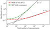 |
Fig. 1. Cost of a likelihood evaluation as a function of the total number of measurements using S+LEAF 2 or the full covariance matrix (see Sect. 5.2). |
In addition to these performances tests, we also ran numerical precision tests. We used the same GP model as for the performances tests and assessed the stability of S+LEAF 2 by computing CC−1x, that is, applying the solving and dot product algorithms on a random merged time series x. In theory, we should find CC−1x = x, however, due to the limited machine precision, numerical errors accumulate and the results stray slightly from x. We computed the root mean square (rms) of these errors, for the S+LEAF 2 methods and for the full covariance matrix (see Fig. 2). In both cases, numerical errors grow with the total number of measurements. However, the level and growth rate are lower when using S+LEAF 2. For a given number of measurements, the number of arithmetic operations is lower when using S+LEAF 2, which could explain the improvement in precision.
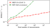 |
Fig. 2. Precision of the linear solving operation as a function of the total number of measurements using S+LEAF 2 or the full covariance matrix (see Sect. 5.2). |
5.3. Periodogram and false alarm probability
We analyzed HD 13808 data using the periodogram and false alarm probability (FAP) approach presented in Delisle et al. (2020a). For each frequency, all the linear parameters (here the RV and indicators offsets) are re-adjusted together with the amplitudes of the cosine and sine at the considered frequency (only applied to the RV time series). The framework of Delisle et al. (2020a) only requires slight adaptations to account for the joint fit of RV and activity indicators, which are detailed in Appendix C.
We first performed a fit of a base model including the offsets γRV, γBIS,  , jitter terms added in quadrature to the measurements errorbars, σRV, σBIS,
  , the kernels hyperparameters, PGP, ρGP, ηGP, and the amplitudes, α, β, by maximizing the likelihood. Then using the fitted noise parameters, we computed a first periodogram, reajusting the offsets for each considered frequency. The resulting periodogram is plotted in Fig. 3 (top). We observe a very significant peak at 14.19 d (FAP = 6.7 × 10⁻²²). We then fitted a Keplerian orbit to this signal, and reajusted all parameters. A second periodogram (Fig. 3, middle) was then computed on the residuals, still reajusting the offsets, but keeping the planetary and noise parameters fixed. A second significant peak is visible at 53.7 d (FAP = 7.7 × 10⁻¹²). As for the first planet, we performed a global fit of all the parameters after including this planet in the model. These fitted parameters are presented in Table 1, the kernel function corresponding to the fitted hyperparameters is illustrated in Fig. 5, and the residuals of each time series superimposed with the GP prediction are shown in Figs. 6 and 7. Finally, the periodogram of the residuals after fitting both planets (Fig. 3, bottom) does not show any significant peak (FAP above 1%). Our conclusions, based on this periodogram and FAP approach, thus agree with the findings of Ahrer et al. (2021), with two confirmed planets at 14.19 d and 53.7 d.
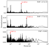 |
Fig. 3. Periodograms of the raw RV time series of HD 13808 (top) as well as of the residuals after subtracting the 14.19 d (center) and the 53.7 d (bottom) planets. |
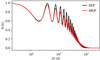 |
Fig. 5. Kernel function used to model HD 13808’s activity (MEP, see Eq. (48)). The GP hyperparameters are taken from the best fit of the two planets solution (Table 1). For comparison, the SEP kernel, which the MEP kernel is design to roughly mimic, is also plotted using the same set of hyperparameters. |
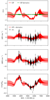 |
Fig. 6. GP prediction (conditional distribution) from the best fit of the two planets solution (Table 1). The prediction is plotted for the GP and its derivative (top) and the full GP prediction for the RV, BIS, and |

Maximum likelihood solution and POLYCHORD posterior for the model with a GP and two planets (at 14.19 and 53.7 d).
We note that the first harmonics part (kSHO, harm.) in the MEP kernel (Eq. (48)) plays a key role in the GP modeling, even if its amplitude is significantly smaller than the fundamental term (kSHO, fund.). Indeed, when neglecting the harmonics term (see Fig. 4), we find a third highly significant signal around 19 d (FAP = 4.3 × 10⁻⁵), which corresponds to half the period of the GP (PGP ≈ 38 d, see Table 1). On the contrary, when including the harmonics part, the peak around 19 d is no more significant (see Fig. 3). This is not surprising since stellar activity is expected to introduce signals in the RV and indicators time series at the rotation period, but also at its harmonics, and, in particular, the first harmonics.
By design, a kernel which has power at the rotation harmonics will have a tendency to absorb signals at this period (here 19 d), even if those are not due to stellar activity. To further test whether the 19 d signal could be due to a planet, Hara et al. (2022a) checked the consistency of this signal over the timespan of the data set. The authors showed that the 19 d signal, while not statistically significant, exhibits a stable presence accross the data set, which might motivate further observations.
5.4. Bayesian framework and false inclusion probability
In order to more directly compare our results with the study of Ahrer et al. (2021), we performed a full Bayesian evidence analysis using the nested sampling algorithm POLYCHORD (Handley et al. 2015). Recently, POLYCHORD was used for radial velocity exoplanet detection by Ahrer et al. (2021), Rajpaul et al. (2021), and Unger et al. (2021). We aimed at reproducing a similar analysis as Ahrer et al. (2021), but using S+LEAF 2 and the GP model detailed in Sect. 5.1.
The prior distributions we used for all parameters are detailed in Table 2. We kept mostly the same priors used by Ahrer et al. (2021), with only a few changes. We set the amplitude for the RV term of the GP to be strictly positive to avoid degeneracies in the sign of the amplitudes. We also shifted the prior for the mean longitudes from [0, 2π] to [ − π, π]. Indeed, the mean longitude of planet c is very close to 0, and this shift avoids splitting the peak in the posterior, thus improving the convergence efficiency. For all runs we used a number of live points equal to 50 ndim, that is, 50 times the number of free parameters. For the precision criterion (stopping criterion), we used 10−9.
Prior distributions used for each parameter in the nested sampling runs with POLYCHORD.
We ran POLYCHORD for models with zero up to three planets and each model was run five times to obtain estimates of the value and uncertainty of the evidence. The evidence for each model is presented in Table 3. We see a steady and significant increase in evidence up to the model with two planets. The two and three planet models present similar evidence (Δln Z = 3.5 ± 2.5, compatible at 1.4σ). Moreover, even if the three planet model is marginally favored, no clear period for a third planet emerges from the posteriors. To illustrate this, we computed the false inclusion probability (FIP) periodogram (Hara et al. 2022b) from the posteriors of all our runs with zero to three planets (see Fig. 8). The true inclusion probability (TIP) provides the probability for the system to host at least one planet in a given (small) range of period. On the contrary, the FIP (=1–TIP) is the probability that the system does not host any planet in the given range of period. The FIP periodogram of Fig. 8 is computed with a window size of 1/(tmax − tmin) in frequency. We observe in Fig. 8 two very significant peaks (FIP less than 10−8) around 14.1 d and 53.7 d, which confirms that these planets should be included in the model. Then, two smaller peaks around 12 d and 19 d are also visible but none of them is significant (FIP higher than 70%). The posterior distribution of parameters of the two-planet runs is given in Table 1. Our results are in agreement with the periodogram and FAP approach detailed in Sect. 5.3, and with Ahrer et al. (2021) findings.
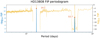 |
Fig. 8. FIP periodogram for HD 13808. In blue we represent the FIP (false inclusion probability) and in yellow the TIP (true inclusion probability). |
Evidence of each considered model in our POLYCHORD runs.
6. Conclusion
In this article, we have presented S+LEAF 2, a GP framework that is able to efficiently model multiple time series simultaneously. Classical GP models have a computational cost that scales as the cube of the number of measurements, which makes them prohibitive in terms of computational resources for large data sets. The computational cost of our GP framework scales linearly with the data set size, which allows for tractable computations even for large data sets.
This work builds on previous studies that provided efficient GP models for single time series (in particular the celerite and S+LEAF models, see Rybicki & Press 1995; Ambikasaran 2015; Foreman-Mackey et al. 2017; Delisle et al. 2020b). It is also inspired by a recent generalization of celerite to the case of two-dimensional data sets (Gordon et al. 2020), but extends it by accounting for the GP derivatives. These derivatives are especially important when modeling the effect of stellar activity on RV time series (see Aigrain et al. 2012; Rajpaul et al. 2015). Our framework additionally accounts for time series that do not share the same calendar, which is useful to train a GP simultaneously on RV and photometric measurements taken with two different instruments (e.g., Haywood et al. 2014).
We applied our methods to reanalyze the RV time series of the nearby K2 dwarf HD 13808. Our results are very similar to a recent state-of-the-art study of the same system (Ahrer et al. 2021) and we confirm the two planets announced in this article. However, we have shown that using our framework allowed us to dramatically decrease (by more than two orders of magnitude) the computational cost of the GP modeling. While the data set analyzed here consists of 738 measurements (RV, BIS, and  at 246 epochs), the gain of using S+LEAF 2 would be even greater for larger data sets. Some data sets (e.g., HARPS or HARPS-N Sun-as-a-star RV time series) that could not have been analyzed with such a GP modeling are now achievable with our GP framework.
Finally, it is worth noting that the results from the periodogram and FAP approach are consistent with the much more computer intensive Bayesian evidence calculations using nested sampling. This illustrates the power of the periodogram and FAP computation including a correlated noise model, as proposed by Delisle et al. (2020a).
Acknowledgments
We thank the referee, D. Foreman-Mackey, for his very constructive feedback that helped to improve this manuscript. We acknowledge financial support from the Swiss National Science Foundation (SNSF). This work has, in part, been carried out within the framework of the National Centre for Competence in Research PlanetS supported by SNSF.
References
- Ahrer, E., Queloz, D., Rajpaul, V. M., et al. 2021, MNRAS, 503, 1248 [NASA ADS] [CrossRef] [Google Scholar]
- Aigrain, S., Pont, F., & Zucker, S. 2012, MNRAS, 419, 3147 [NASA ADS] [CrossRef] [Google Scholar]
- Ambikasaran, S. 2015, Numer. Linear Algebra Appl., 22, 1102 [CrossRef] [Google Scholar]
- Baluev, R. V. 2008, MNRAS, 385, 1279 [Google Scholar]
- Blackman, R. T., Fischer, D. A., Jurgenson, C. A., et al. 2020, AJ, 159, 238 [CrossRef] [Google Scholar]
- David, T. J., Petigura, E. A., Luger, R., et al. 2019, ApJ, 885, L12 [Google Scholar]
- Delisle, J. B., Hara, N., & Ségransan, D. 2020a, A&A, 635, A83 [NASA ADS] [CrossRef] [EDP Sciences] [Google Scholar]
- Delisle, J. B., Hara, N., & Ségransan, D. 2020b, A&A, 638, A95 [EDP Sciences] [Google Scholar]
- Dumusque, X., Udry, S., Lovis, C., Santos, N. C., & Monteiro, M. J. P. F. G. 2011, A&A, 525, A140 [NASA ADS] [CrossRef] [EDP Sciences] [Google Scholar]
- Dumusque, X., Pepe, F., Lovis, C., et al. 2012, Nature, 491, 207 [Google Scholar]
- Foreman-Mackey, D. 2018, Res. Notes Am. Astron. Soc., 2, 31 [NASA ADS] [Google Scholar]
- Foreman-Mackey, D., Agol, E., Ambikasaran, S., & Angus, R. 2017, AJ, 154, 220 [Google Scholar]
- Gillen, E., Briegal, J. T., Hodgkin, S. T., et al. 2020, MNRAS, 492, 1008 [Google Scholar]
- Gordon, T. A., Agol, E., & Foreman-Mackey, D. 2020, AJ, 160, 240 [NASA ADS] [CrossRef] [Google Scholar]
- Handley, W. J., Hobson, M. P., & Lasenby, A. N. 2015, MNRAS, 453, 4384 [Google Scholar]
- Hara, N. C., Delisle, J.-B., Unger, N., & Dumusque, X. 2022a, A&A, 658, A177 [NASA ADS] [CrossRef] [EDP Sciences] [Google Scholar]
- Hara, N. C., Unger, N., Delisle, J.-B., Díaz, R., & Ségransan, D. 2022b, A&A, accepted, https://doi.org/10.1051/0004-6361/202140543 [Google Scholar]
- Haywood, R. D., Collier Cameron, A., Queloz, D., et al. 2014, MNRAS, 443, 2517 [Google Scholar]
- Jones, D. E., Stenning, D. C., Ford, E. B., et al. 2017, ArXiv e-prints [arXiv:1711.01318] [Google Scholar]
- Jordán, A., Eyheramendy, S., & Buchner, J. 2021, Res. Notes Am. Astron. Soc., 5, 107 [Google Scholar]
- Mayor, M., Marmier, M., Lovis, C., et al. 2011, ArXiv e-prints [arXiv:1109.2497] [Google Scholar]
- Noyes, R. W., Hartmann, L. W., Baliunas, S. L., Duncan, D. K., & Vaughan, A. H. 1984, ApJ, 279, 763 [Google Scholar]
- Pepe, F., Cristiani, S., Rebolo, R., et al. 2021, A&A, 645, A96 [NASA ADS] [CrossRef] [EDP Sciences] [Google Scholar]
- Queloz, D., Henry, G. W., Sivan, J. P., et al. 2001, A&A, 379, 279 [NASA ADS] [CrossRef] [EDP Sciences] [Google Scholar]
- Rajpaul, V., Aigrain, S., Osborne, M. A., Reece, S., & Roberts, S. 2015, MNRAS, 452, 2269 [Google Scholar]
- Rajpaul, V. M., Buchhave, L. A., Lacedelli, G., et al. 2021, MNRAS, 507, 1847 [NASA ADS] [CrossRef] [Google Scholar]
- Rasmussen, C. E., & Williams, C. K. I. 2006, Gaussian Processes for Machine Learning (MIT Press) [Google Scholar]
- Rybicki, G. B., & Press, W. H. 1995, Phys. Rev. Lett., 74, 1060 [NASA ADS] [CrossRef] [Google Scholar]
- Unger, N., Ségransan, D., Queloz, D., et al. 2021, A&A, 654, A104 [NASA ADS] [CrossRef] [EDP Sciences] [Google Scholar]
Appendix A: Semiseparable representation of Matérn 3/2 and Matérn 5/2 kernels
The Matérn 3/2 and 5/2 covariances are widely used in various fields of statistics. Their kernel functions are written as
where x is the rescaled time:
and σ and ρ are the GP hyperparameters.
A.1. Semiseparable representation
For two times ti > tj, we have

which provides the semiseparable representation of rank 2
for the Matérn 3/2 kernel. Similarly, the Matérn 5/2 kernel admits the semiseparable representation of rank 3
These representations are not unique and the choice of splitting into the 2 (Matérn 3/2) or 3 (Matérn 5/2) semiseparable terms is arbitrary.
A.2. Derivative of a Matérn Gaussian process
A GP following the Matérn 3/2 or 5/2 kernel is always differentiable, independently of the hyperparameters. Following the same reasoning as in Sect. 3, we compute the derivatives of U and V, as well as the matrix B, which appear in the covariance matrix between the GP G(t) and its derivative G′(t) and in the covariance matrix of G′(t) itself (see Eq. (22)). We find
for the Matérn 3/2 kernel, and
for the Matérn 5/2 kernel.
A.3. Overflows and preconditioning
To avoid overflows (see Sect. 4.4), these representations can be adapted to use the same preconditioning method as in the case of the classical celerite quasiperiodic terms. The preconditioning matrix ϕ is defined as
and the preconditioned matrices  ,
,  ,
,  , and
, and  are obtained by dropping the exponential terms from the definitions of U, V, U′, and V′. For instance, we have
for the Matérn 3/2 covariance matrix.
While this preconditioning allows us to prevent overflows and underflows due to the exponential terms, weaker numerical instabilities could arise due to the presence of xi and  in the definitions of the preconditioned matrices. The absolute values of the rescaled times xi should thus be kept as small as possible to improve numerical stability. Since the Matérn kernels are stationary (i.e., k only depends on Δt), a reference time t0 can be chosen arbitrarily, and the definition of x (Eq. (A.2)) can be adapted accordingly
For instance, we could use
to avoid xi values that are too large. This might not be sufficient for a very large time span compared to the decay timescale, ρ; particularly in the case of the Matérn 5/2 kernel, which contains quadratic terms ( ). Recently, Jordán et al. (2021) proposed a state-space representation for the Matérn 3/2 and 5/2 kernels, which allows a similar linear scaling of the likelihood evaluation with improved numerical stability.
Appendix B: Twice mean square differentiable semiseparable kernels
In this appendix we construct several twice mean square differentiable semiseparable kernels. When modeling time series as combinations of a GP and its derivative, the chosen GP kernel must at least be once mean square differentiable for the model to be valid. However, using a twice mean square differentiable kernel ensures that the GP’s derivative is itself differentiable, which typically generates smoother models.
B.1. Alternatives to the SE kernel
The Matérn 5/2 kernel is a widely spread kernel which has the advantage of being both twice differentiable and semiseparable with rank r = 3 (see Appendix A). If twice differentiability is required, it is thus a natural alternative to the squared-exponential (SE) kernel:

since the latter cannot be modeled with celerite/S+LEAF. Higher order Matérn kernels, such as the Matérn 7/2 kernel could also be used as they are more than twice differentiable and admit semiseparable representations. However, the rank of their semiseparable representations would be higher, which would increase the cost of likelihood evaluations.
We additionally propose here the exponential-sine (ES) kernel
which is also twice differentiable and semiseparable with rank 3. Its cost is thus similar to the Matérn 5/2 kernel. The corresponding power spectral density (PSD)
is always positive (for λ > 0), which ensures the positive definiteness of the kernel (e.g., Foreman-Mackey et al. 2017). The parameters λ and μ can be chosen arbitrarily, but using

makes the deviation between the SE and the ES kernels below 0.009σ2 for all lags Δt. Figure B.1 illustrates this by comparing the SE, ES, and Matérn 5/2 kernels and PSD.
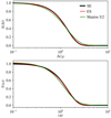 |
Fig. B.1. Comparison of the kernel functions (top) and power spectral density (bottom) of the SE, ES, and Matérn 5/2 kernels. The timescale of the Matérn 5/2 kernel is adjusted such as to minimize the maximum deviation from the SE kernel. |
B.2. Alternatives to the SEP kernel
As seen in Eq. (46) the SEP kernel can be approximated by
In this expression, the periodic part
is semiseparable and verifies  . Thus, in order to obtain a twice differentiable semiseparable kernel similar to the SEP kernel, we simply need to replace the SE part in Eq. (B.5) by a Matérn 5/2 or ES kernel and we define


Indeed, the product of two semiseparable terms is semiseparable (see Foreman-Mackey et al. 2017) and since
the first and third derivatives of k5/2P and kESP also cancel out at Δt = 0. The PSD of these two kernels are given by
where k = 5/2 or ES. Since the PSD (Sk) of the Matérn 5/2 and ES kernels are strictly positive for all frequencies and the coefficient f = (2η)−2 is strictly positive, we find that S5/2P and SESP are also strictly positive for all frequencies. The two corresponding kernels are thus positive definite.
The rank of the semiseparable representations of k5/2P and kESP is r = 15, since they are the product of a rank 3 kernel (Matérn 5/2 or ES) and a rank 5 kernel (periodic part). As a comparison, the MEP kernel (see Eq. 48), which is not twice differentiable, is of a rank of 6.
We reproduced the analyses of Sects. 5.2 and 5.3 using the ESP kernel instead of the MEP kernel. The results are presented in Figs. B.2–B.6. The cost of likelihood evaluations using the ESP kernel is about twice the cost of using the MEP kernel (see Fig. B.2), which is still much more efficient than modeling the full covariance matrix. The periodograms (Fig. B.3), as well as the GP prediction (Figs. B.4 and B.5) are very similar to the ones obtained with the MEP kernel (Figs. 3, 6, and 7). Finally, we see in Fig. B.6 that the ESP kernel reproduces the SEP kernel very closely while the MEP kernel mimics it more roughly (see Fig. 5). However, these differences between the MEP and the ESP (or SEP) kernels seem to have a very weak impact on our analysis, since the periodograms and GP prediction are similar in both cases.
Appendix C: Periodogram and FAP for heterogeneous time series
We consider here the case of an heterogeneous time series following Eq. (28) and we are aimed at detecting a periodic signal affecting the first time series Y1 only. The frameworks of Baluev (2008) and Delisle et al. (2020a) defining a general class of linear periodograms with their associated analytical FAP approximations can be applied to the merged time series y of Eq. (31) with a slight modification. We thus refer to Delisle et al. (2020a) for the details of the framework and we focus here on the required adaptations. Following Delisle et al. (2020a), we compare the χ2 of a linear base model ℋ of p parameters with enlarged models 𝒦 of p + d parameters, parameterized by the frequency ν. The base model is defined as

where θℋ is the vector of size p of the model parameters, φℋ is a n × p matrix, and n the total number of points in the merged time series y. The columns of φH are explanatory time series that are scaled by the linear parameters θℋ. For instance, if we consider the merged time series of RV, BIS, and  , and we include in the model an offset for each of these time series, we would have to define:

where γi is the offset of time series i, and δi is equal to one for measurements belonging to time series i and zero otherwise. The matrix φℋ would thus be a n × 3 matrix, whose first column would be filled with 1 for RV measurements and 0 otherwise, the second column would be equal to 1 for BIS measurements, and the last column for  measurements. The vector of parameters would then be
  .
.
The enlarged model 𝒦(ν) is written as

where θ𝒦 = (θℋ, θ) is the vector of size p + d of the parameters and φ𝒦(ν) = (φH, φ(ν)) is a n × (p + d) matrix whose p first columns are those of φℋ, and whose d last columns are functions of the frequency, ν. In the case of an homogeneous time series, as in Delisle et al. (2020a), one typically uses φ(ν) = (cos(νt), sin(νt)) (with d = 2). The main difference in the case of heterogeneous time series is that we only search for a periodicity in the first time series (Y1, typically the RV time series). Thus, we would define φ(ν) = (cos(νt)δ1, sin(νt)δ1). All the results presented in Delisle et al. (2020a) remain valid when applied to the merged time series. The only difference is that due to the presence of zeroes in φ for all measurements not belonging to the first time series, the averaging used in the definition of the effective time series length (Delisle et al. 2020a Eq. (8)) is restricted to the first time series measurements
where C−1 is the inverse of the full covariance matrix of the merged time series.
All Tables
Maximum likelihood solution and POLYCHORD posterior for the model with a GP and two planets (at 14.19 and 53.7 d).
Prior distributions used for each parameter in the nested sampling runs with POLYCHORD.
All Figures
|
Fig. 1. Cost of a likelihood evaluation as a function of the total number of measurements using S+LEAF 2 or the full covariance matrix (see Sect. 5.2). |
| In the text | |
|
Fig. 2. Precision of the linear solving operation as a function of the total number of measurements using S+LEAF 2 or the full covariance matrix (see Sect. 5.2). |
| In the text | |
|
Fig. 3. Periodograms of the raw RV time series of HD 13808 (top) as well as of the residuals after subtracting the 14.19 d (center) and the 53.7 d (bottom) planets. |
| In the text | |
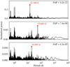 |
Fig. 4. Same as Fig. 3 but neglecting the harmonics component of the MEP kernel (see Eq. (48)). |
| In the text | |
|
Fig. 5. Kernel function used to model HD 13808’s activity (MEP, see Eq. (48)). The GP hyperparameters are taken from the best fit of the two planets solution (Table 1). For comparison, the SEP kernel, which the MEP kernel is design to roughly mimic, is also plotted using the same set of hyperparameters. |
| In the text | |
|
Fig. 6. GP prediction (conditional distribution) from the best fit of the two planets solution (Table 1). The prediction is plotted for the GP and its derivative (top) and the full GP prediction for the RV, BIS, and |
| In the text | |
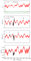 |
Fig. 7. Zoom of Fig. 6 around epoch 2 453 720 BJD. |
| In the text | |
|
Fig. 8. FIP periodogram for HD 13808. In blue we represent the FIP (false inclusion probability) and in yellow the TIP (true inclusion probability). |
| In the text | |
|
Fig. B.1. Comparison of the kernel functions (top) and power spectral density (bottom) of the SE, ES, and Matérn 5/2 kernels. The timescale of the Matérn 5/2 kernel is adjusted such as to minimize the maximum deviation from the SE kernel. |
| In the text | |
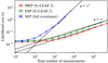 |
Fig. B.2. Same as Fig. 1 but including the ESP kernel in the performance comparison. |
| In the text | |
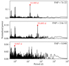 |
Fig. B.3. Same as Fig. 3 but using the ESP kernel instead of the MEP kernel. |
| In the text | |
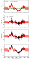 |
Fig. B.4. Same as Fig. 6 but using the ESP kernel instead of the MEP kernel. |
| In the text | |
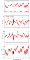 |
Fig. B.5. Same as Fig. 7 but using the ESP kernel instead of the MEP kernel. |
| In the text | |
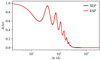 |
Fig. B.6. Same as Fig. 5 but using the ESP kernel instead of the MEP kernel. |
| In the text | |
Current usage metrics show cumulative count of Article Views (full-text article views including HTML views, PDF and ePub downloads, according to the available data) and Abstracts Views on Vision4Press platform.
Data correspond to usage on the plateform after 2015. The current usage metrics is available 48-96 hours after online publication and is updated daily on week days.
Initial download of the metrics may take a while.