| Issue |
A&A
Volume 659, March 2022
|
|
|---|---|---|
| Article Number | A63 | |
| Number of page(s) | 12 | |
| Section | Interstellar and circumstellar matter | |
| DOI | https://doi.org/10.1051/0004-6361/202141258 | |
| Published online | 07 March 2022 | |
Completing the X-ray view of the recently discovered supernova remnant G53.41+0.03★
1
Anton Pannekoek Institute for Astronomy, University of Amsterdam,
Science Park 904,
1098 XH
Amsterdam, The Netherlands
e-mail: vdomcek@gmail.com
2
GRAPPA, University of Amsterdam,
Science Park 904,
1098 XH
Amsterdam, The Netherlands
3
SRON, Netherlands Institute for Space Research,
Utrecht, The Netherlands
4
School of Astronomy and Space Science, Nanjing University,
Nanjing
210023,
PR China
5
Jodrell Bank Centre for Astrophysics, School of Physics and Astronomy, The University of Manchester,
Manchester,
M13 9PL, UK
Received:
6
May
2021
Accepted:
7
January
2022
Aims. We present a detailed X-ray study of the recently discovered supernova remnant (SNR) G53.41+0.03, which follows up and further expands on the previous, limited analysis of archival data covering a small portion of the SNR.
Methods. With the new dedicated 70 ks XMM-Newton observation we investigate the morphological structure of the SNR in X-rays, search for a presence of a young neutron star, and characterise the plasma conditions in the selected regions by means of spectral fitting.
Results. The first full view of SNR G53.41+0.03 shows an X-ray emission region well aligned with the reported half-shell radio morphology. We find two distinct regions of the remnant that differ in terms of the brightness and hardness of the spectra, and both regions are best characterised by a hot plasma model in a non-equilibrium ionisation state. Of the two regions, the brighter one contains the most mature plasma, with ionisation age τ ≈ 4 × 10¹⁰ s cm−3 (where τ = net), a lower electron temperature of kTe ≈ 1 keV, and the highest estimated gas density, nH ≈ 0.87 cm−3. The second, fainter but spectrally harder, region reveals a younger plasma (τ ≈ 1.7 × 10¹⁰ s cm−3) with a higher temperature (kTe ≈ 2 keV) and a two to three times lower density (nH ≈ 0.34 cm−3). No clear evidence of X-ray emission was found for emission from a complete shell, the southern part appearing to be absent. Employing several methods for age estimation, we find the remnant to be t ≈ 1000–5000 yr old, confirming earlier reports of a relatively young age. The environment of the remnant also contains a number of point sources, most of which are expected to be positioned in the foreground. Of the two point sources in the geometrical centre of the remnant, one is consistent with the characteristics of a young neutron star.
Key words: ISM: supernova remnants / ISM: individual objects: G53.41+0.03 / stars: neutron
The data underlying this article are available in the zenodo repository, at https://doi.org/10.5281/zenodo.4737383
© ESO 2022
1 Introduction
Supernova remnants (SNRs) are an important link in the cycle of gas in galaxies, connecting star formation, stellar deaths, and galactic chemical evolution. Moreover, the mechanical energy provided by supernovae (SNe) is transferred to the interstellar gas by SNR shocks, which is an important ingredient for star formation (Kim & Ostriker 2015; Koo et al. 2020). Supernova remnants provide insights into the final stage of the lives of massive stars since their shock waves illuminate the late mass loss history of the SN progenitors, and their compositions, enhanced by freshly synthesised elements, reveal details about the explosion mechanism and progenitor properties. Early on, after the explosion, they provide favourable conditions for dust condensation, and their shock waves are thought to be the dominant producers of Galactic cosmic rays (Vink 2020). The interaction of the shocks and the mixing of the SN-produced elements with the interstellar medium (ISM) lead to its chemical enhancement, thus providing SN feedback to the Galaxy. There is, therefore, a considerable interest in completing our view of the Galactic SNR population.
With the next generation of Galactic surveys in both radio – for example, THOR (The H1/OH/Recombination line) survey (Anderson et al. 2017) and the LOFAR (LOw Frequency ARray) Two-metre Sky Survey (Shimwell et al. 2017) – and X-rays – for example, eROSITA (Merloni et al. 2012) – there has been a renewed interest in finding new SNRs. The reason is the still relatively low number of identified SNRs (~294 in Green 2019 and ~384 in Ferrand & Safi-Harb 2012) compared to the expected 2000–3000 estimated from the Galactic SN rate (Vink 2020).
G53.41+0.03 is one of the recently found SNRs that came out of the mapping of the relatively crowded field along the Sagittarius-Carina and Perseus arms of the Galaxy. It appeared as a candidate SNR in the THOR survey (Anderson et al. 2017), and the measured radio spectral index of α ≈−0.6 (for Sv ∝ να) from a LOFAR wide field investigation (Driessen et al. 2018) confirmed its SNR nature. A portion of the remnant was covered by an archival XMM-Newton observation at the edge of one of its MOS detectors. An analysis of this partial dataset proved the existence of a hot non-equilibrium ionisation (NEI) plasma coinciding with the radio emission, further confirming the SNR nature of G53.41+0.03 and hinting at a relatively young age of the remnant for the estimated distance of about 7.5 kpc (Driessen et al. 2018).
In this work, we follow up on SNR G53.41+0.03 with a new dedicated 70 ks XMM-Newton observation. We provide a first complete look at the morphology in X-rays and analyse three distinct regions of the remnant. We characterise the plasma conditions in these regions with an aim to provide a better understanding of the local plasma characteristics and more precisely estimate the age of the remnant. We also discuss potential neutron star candidates seen in the SNR’s geometrical centre.
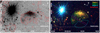 |
Fig. 1 SNR G53.41+0.03 with a type I outburst of the high mass X-ray binary IGR J19294+1816 in October 2019. Left: grey-scale image in the energy range 0.8–4.0 keV. Radio contours of the THOR VGPS survey (Anderson et al. 2017) with levels –(0.013, 0.01475, 0.02) Jy beam−1 are overlaid on top of the X-ray data. Right: three-colour image (red 0.8–1.5 keV, green 1.5–2.5 keV, and blue 2.5–4.0 keV) of the extraction and exclusion regions used in the analysis. We applied square-root scaling to the left image and logarithmic scaling to the right image to improve visibility. |
XMM-Newton observations used in this work.
2 Observations and data reduction
We performed a dedicated 70 ks XMM-Newton observation of the SNR G53.41+0.03 on 13 October 2019 (ObsID: 0841190101, PI: Domček). We used the new dataset together with the archival one (ObsID: 0503740101, PI: Wang), which encompasses only part of the remnant at the edge of the field of view (FoV) of one of the detectors (Driessen et al. 2018). The list of the used observationsis provided in Table 1.
We extracted images and spectra with the Science Analysis System (SAS) v18.0. The tasks epchain and emchain were used for the data reduction, and pn-filter and mos-filter were employed for filtering the background flaring. This resulted in clean exposures times of 52 ks for MOS1, 65 ks for MOS2 (though 32 ks in the case of the 2008 observation), and 42 ks for pn in the case of the 2019 observation. Tasks eimageget and eimagecombine were used in order to obtain the image of the remnant in Fig. 1. We used XSPEC (12.11.1) (Arnaud 1996) for our spectral analysis and modelling. We employed C-statistics (Cash 1979) and the optimal binning method ftgrouppha (Kaastra & Bleeker 2016), which is part of the Heasoft package1.
Throughout the 2019 observation, a type I outburst from a nearby high mass X-ray binary was detected in the same FoV (Domcek et al. 2019). This caused an unexpected contamination of the SNR region. The problems are mainly present in the pn detector, although the MOS chips required the exclusion of the affected regions as well. For that reason we focused our analysis on the higher spectral resolution MOS spectra.
3 Results
3.1 Morphology of the remnant
SNR G53.41+0.03 has a half-shell morphology of 3.5′ in size with most of the emission coming from the upper half (in Galactic coordinates), as shown in Fig. 1. The lower half of the SNR does not show any clear morphological detection in Fig. 1. The SNR is located in an environmentwith several point sources in the line of sight. Two of these are particularly interesting as they are positioned in the assumed geometric centre of the remnant. We discuss their properties and relation to the remnant further in Sect. 4.3.
3.2 Spectral analysis
For our spectroscopic analysis, we divided the SNR into three regions based on the morphology and hardness of the spectra (see Fig. 1, right). Region 1 was selected in the top part of the SNR, where the X-ray emission is brightest and its spectrum also appears softest. This region spatially coincides with the region previously analysed by Driessen et al. (2018). Region 2 is positioned in the previously unobserved part of the remnant. This section is fainter and has a harder spectrum compared to region 1. Region 3 does not show obvious emission in the X-ray map but fills the spherical structure of the remnant. All three regions plus the background modelling region are shown in Fig. 1 (right).
We fitted all background spectra in the wider 0.3–10 keV range, while the 0.5–10 keV energy range was used for the spectra of source regions. Uncertainties are reported in the 1σ confidence range and are calculated through the Markov chain Monte Carlo (MCMC) method, utilising the Goodman–Weare algorithm (Goodman & Weare 2010) with 600 walkers and 106 steps. The results of the MCMC runs are also provided in Figs. A.1–A.3, and B.1.
3.2.1 Background modelling
We modelled the extracted MOS1 and MOS2 backgrounds using a combination of the models TBabs, Apec, and Power-law2 and several Gaussian lines. The Gaussian lines represent the instrumental background lines, and their normalisation is left to vary even for the source spectra due to their non-flat distribution across the detector. More details on the background model components are available in Masui et al. (2009) and Sun & Chen (2020).
The parameters of these model components are, apart from the normalisation of the Gaussians, linked together for all of the MOS spectra in use. We obtained an acceptable fit with C-stat/d.o.f. of 306/247. The spectrum together with the model are shown in the top-left panel of Fig. 2. This background model, scaled to the extraction area, was applied to all the subsequent MOS spectra, except for the central point source analysis, which has a separate background model treatment.
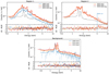 |
Fig. 2 Best-fit models for the source and the background region spectra. A black dashed line shows the MOS 2 detector background model for individual regions. In region 2 we display the best-fit model fitted in the 0.5–5.0 keV energy range. |
3.2.2 Region 1
The spectrum is well represented with a single NEI plasma model, vnei3 (Borkowski et al. 2001), with the abundances of Ne, Mg, Si, S, and Fe released. The best-fit values with 329/277 (C-stat/d.o.f.) show the plasma temperature to be 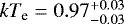 keV, the ionisation age to be
 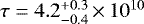 s cm−3, and mostly solar abundances, which is consistent with the previous findings for this particular region. The total number of counts for this region, including the background, is ~19200 ct.
3.2.3 Region 2
Region 2 is positioned in the previously uncovered northern part of the remnant and, therefore, only MOS1 and MOS2 spectra from the 2019 observation are available. Applying the non-equilibrium model TBabs*vnei reproduces the spectrum well with the fit statistics of 197/171 (C-stat/d.o.f.). Although the plasma temperature is expected to be higher based on the hardness of the three-colour image, the fitted temperate,  keV, is still rather high.
We suspect that the higher temperature compared to region 1 could be a flux excess in the spectrum around 5–6 keV (see the lower-left panel of Fig. 2). We considered two explanations for this excess: (i) a physical interpretation, which would explain the excess with non-thermal emission coming out of this part of the SNR; or (ii) a technical interpretation, where the reason for the excess could be explained with a local calibration or background issue.
For the first scenario, we included an additional power-law component with Γ = 3 in our model. We obtained a marginally better fit to the data with 191/170 (C-stat/d.o.f.). However, the plasma temperature 1σ confidence range increased to an even higher, and less probable,  keV. Additionally, releasing the power-law index lead to a preferred value of Γ ≈ 0.3, a value that is not consistent with the range of values known for the non-thermal emission in SNRs, as reported for example in Table 3 of Sasaki et al. (2004).
The alternative explanation is contamination from a quiescent particle background, where Cr and Mn lines are known to be present in this energy range (Kuntz & Snowden 2008, see Figs. 2 and 3). We therefore restricted the fit to data in the energy range 0.5–5.0 keV, where the SNR’s emission clearly dominates. The fit statistic in this case was 86/104 (C-stat/d.o.f.), with the fitted temperate moving to a lower estimate of  keV. The best-fit ionisation age is
  s cm−3, and abundances stay roughly solar and similar for both energy ranges. Full details on the fitted models can be found in Table 2. The total number of counts for this region, including the background, is ~4200 ct.
Best-fit values for two selected regions of the remnant.
3.2.4 Region 3
The spectrum of region 3 does show a minor surplus of emission above the background model, mainly in the 1.2–1.4 keV energy range. However, considering the faintness of the emission and the variability in the background across the FoV, we do not find sufficient evidence for significant detection. The total number of counts for this region, including the background, is ~5100 ct.
4 Discussion
Previous work by Driessen et al. (2018) confirmed the presence of an X-ray-emitting plasma coinciding with the location of a radio structure that could be explained only by SNR shocks. The probable location of the remnant was placed at the outer edge of the Sagittarius-Carina Arm, at a distance of approximately 7.5 kpc. Using various age estimation techniques, the age of the SNR was estimated to be between 1000 and 8000 yr. With the newly acquired dataset, we build upon the previous results and provide a more complete picture of the remnant.
4.1 Visible structure of the SNR
A full view of G53.41+0.03 shows a half-spherical X-ray morphology with the size of the remnant somewhat smaller (θX ~ 3.5′) than the size estimated in the radio band (θR ~ 5′). However, the difference in the size estimate is most likely caused by a better image resolution in the X-ray band and not by a different morphology. We can therefore now confirm that the overall X-ray morphology aligns well with the visible radio structure.
The more accurate measurements of the SNR’s angular size result in updates of the previously reported characteristics (Driessen et al. 2018), such as estimates of physical size, number densities, and the plasma age. For the distance estimate of d ≈ 7.5 kpc (Driessen et al. 2018), the physical radius of the SNR is r ~ 7.64d7.5 pc, where d7.5 = d∕7.5 kpc.
As mentioned in Sect. 3.1, the two regions selected for further analysis differ in terms of brightness and spectral characteristics. These differences are likely caused by density variations in the SNR and its ambient medium. We tested this idea by estimating the number densities in those regions.
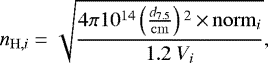
In order to calculate the number densities for the individual regions (nH,i), we used
 (1)
(1)
where normi = (10−14∕4πD2)∫ nenHdV is a normalisation per region4, d7.5 is the distance to the SNR, and Vi is the volume of emitting plasma. We took ne = 1.2nH to account for the electron number densities, ne, released by the ionisation of hydrogen atoms.
To estimate the total volume of the emitting plasma, we assumed a Sedov remnant with a shock compression ratio of χ ~ 4. The volume-filling factor in that case is ~ 25% (e.g. Reynolds 2017), leading to an estimate of 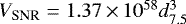 cm3. The total volume is distributed in individual regions according to their size (Table 3).
The calculated particle densities show, unsurprisingly, that the brighter region 1 also has a higher density. Region 1 consists of material that is two to three times denser compared to region 2 (Table 3). This leads to faster particle interaction and cooling, and hence stronger X-ray emission. In this scenario we could also expect the plasma in region 1 to be more mature, with higher values of τ and lower temperaturekTe due to the plasma cooling efficiency. This is indeed what we see in Table 2.
A possible reason for the difference in densities could be that it arises from an asymmetry in the stellar wind of the progenitor star caused by the movement of the star with respect to the local ISM. This idea was originally proposed byWeaver et al. (1977) and has been evoked, for example, in the case of RCW 86 (Vink et al. 1997). More recenttwo-dimensional simulations of wind bubbles produced by runaway stars have been calculated by, among others, Meyer et al. (2015). The authors show an explosion of an SN in an asymmetric bubble environment and predict that while the SNR explosion wave reaches accumulated matter of the bow shock within the first ~ 1000 yr, the collision with the rest of the cavity border continues for several thousand years afterwards. Although specific progenitor star parameters might differ, we could nevertheless be observing the second stage of this scenario, in which the shock wave has already reached the bow shock over-density and is just now expanding through the lower density cavity border. Another alternative could be an ISM enhancement unrelated to the evolution of the progenitor star.
The stellar wind asymmetry model or the ISM enhancement could explain why regions 2 and 3 show much fainter or no emission compared toregion 1, though it might not be the only reason for the visual distinction. For example, region 3 also lies much closer to the galactic plane and thus experiences much higher line of sight absorption, as indicated by the higher measured hydrogen column density, NH. This is supported by the presence of the infrared dark cloud (IRDC) G53.2 with associated CO emission at a distance of 1.7 kpc (Kim et al. 2015, Figs. 3 and 9).
Volume of emitting plasma, number density, and plasma age estimates for regions in SNR G53.41+0.03.
4.2 Age of the remnant
There are several approaches to estimating the age of X-ray-emitting plasma in SNRs. The most widely used ones are either motivated by the Sedov–Taylor self-similar evolution model or based on the degree of ionisation non-equilibration of elements with prominent emission lines. We discuss both methods here.
4.2.1 Sedov–Taylor model
In the Sedov–Taylor approach, the plasma age can be estimated from the fitted parameter of the post-shock electron temperature, kTe. Under the assumption of full equilibrium of electron and ion temperatures, kTe ties to the shock velocity, vsh, as
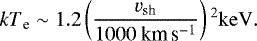 (2)
(2)
The obtained shock velocity is further related to the plasma age, tv, through the Sedov–Taylor model as
 (3)
(3)
where r is the size of the remnant. It should be noted that the measured Te and the post-shock proton temperature, Tp, which dominates the internal energy of the plasma, are not necessarily the same. Vink et al. (2015) showed how the ratio β =Te∕Tp depends on the shock’s Mach number and, in the case of the SNRs, can range from β =0.05 to 1.0. Lower β values can result in lower age estimates by a factor  . For comparison, Sasaki et al. (2004) used β = 0.4 in the case of the more mature CTB 109. If we used β = 0.3 for a presumably younger G53.41+0.03, tv estimates in Table 3 would be around half of those calculated for the full equilibrium.
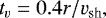
Another independent age estimate based on the Sedov-Taylor model depends on the SNR’s radius, R, the pre-shock density, ρ = (nH∕χ) × mp, where χ is a shock compression ratio, and the explosion energy, E,
 (4)
(4)
We used the updated radius R = 7.64 pc and canonical explosion energy E = 1051 erg. The post-shock number densities, nH (Table 3), are converted into the pre-shock densities required for this calculation by assuming a strong shock compression ratio of χ = 4. The resulting pre-shock densities are used as lower and upper bounds for the age estimation. We find the age to be in the range tE ~ 850–1350 yr. It is likely that the average estimate lies somewhere in between these two values.
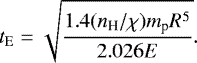
4.2.2 Ionisation age
The ionisation age, τ, is a measure of ionisation non-equilibrium in a plasma. It is a product of the plasma (number) density, ne, and the time since the material has been shocked, tτ. Given the estimates of nH provided in Table 3, and using our previous assumption of ne = 1.2nH, we can obtain another independent estimate of the plasma age based on tτ = τ∕ne.
However, the SNR shell contains plasma shocked fairly recently, at t ≈ 0, as well as plasma that was shocked not long after the SN explosion. Moreover, during the expansion the density changes, so for a given plasma element what counts is τ = ∫ ne(t)dt. The measured τ characterises the bulk of the plasma ionisation age and is necessarily smaller than the maximum possible  , with
  being the current age of the SNR. Borkowski et al. (2001) reported that in the case of the Sedov–Taylor model with the uniform ambient ISM distribution, the most common τ within the shell is τ ≈ 0.3τ0.
The conversion of τ to age is dependent on the density distribution around the SNR, which is likely affected by the mass loss history of the SNR progenitor. For example, a stable stellar wind has ρ ∝ r−2, leading to a higher density near the explosion centre (and hence a larger τ) if we compare the age and the density near the shock radius.
The two regions (1 and 2) show a consistent picture in terms of the age of the shocked plasma, which is around  kyr. To understand the range of allowed ages, we produced contour plots between the emission measure (
 normi) and ionisation age (τ), shown in Fig. 3. We overlaid these figures with curves that represent constant time as prescribed by
 (5)
(5)
where t represents the age of the remnant and EMi is emission measure ∫ nenHdV. These figures further constrain the age of the plasma to  kyr for region 1 and
  kyr for region 2 (in the 1σ range).
All of the estimation techniques used here have some caveats, which makes pinpointing the exact age of SNRs difficult. However, combining all calculated estimates from regions 1 and 2 portrays a mostly consistent picture of the material having been shocked around ~ 1000–5000 yr ago. This estimate puts G53.41+0.03 itself into a similar age range, and thus into the category of younger SNRs. The calculated extinction using Fig. 3 of Predehl & Schmitt (1995) points to a high Av ~ 15 mag, which would make it invisible to the observers of that time.
The range of possible ages calculated above deviates somewhat from the estimates reported in Driessen et al. (2018), which were based on a larger estimate of the radius. Moreover, Driessen et al. (2018) did not correct for the fact that the ionisation age  for SNRs expanding in a uniform medium, with
  giving the current age of the SNR.
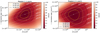 |
Fig. 3 Two-dimensional contour plots of emission measure vs. ionisation age, τ. Dashed linesrepresent curves of the same (τ∕ne) prescribed by Eq. (5). |
4.3 Point sources in the FoV
The proximity to the Galactic plane and the location within the Sagittarius–Carina Arm suggest that the SNR has a core-collapse origin. But a final confirmation needs a proper identification of one of the point sources as the stellar remnant, or more accurate abundance measurements associated with an ejecta component. The FoV around the SNR provides a number of point sources. Many of them are likely associated with the IRDC G53.2 and lie in the foreground of the SNR at a distance of ~ 1.7 kpc. Kim et al. (2015) identified ~370 point sources, ~300 of which are young stellar object (YSO) candidates. We concentrate mainly on the study of the SNR, and we therefore did not conduct a detailed investigation of all of them. However, the point sources in the assumed geometrical centre of the SNR provide an intriguing hypothesis: they could be related to the SNR as its leftover co-created neutron star. We therefore examined these point sources in more detail.
As the first step, we compared the positions of two point source locations, PS1 (RA 19:29:56.0, Dec +18:10:19.2) and PS2 (RA 19:29:54.3, Dec +18:10:23.5), with the list of known YSOs from Kim et al. (2015) and other potential SIMBAD-registered sources. While the PS1 location (the lower of the two in Fig. 1) did not provide any catalogued object within 24″, PS2 lies within 3″ of a YSO identified as 2MASS J19295440+1810260. As this is within the resolving power of XMM-Newton (spatial resolution of 6″ at 1keV) and YSOs are known X-ray emitters (Giardino et al. 2007; Winston et al. 2010), they are most likely the same object and not associated with the SNR.
To further investigate whether the PS1 central source could be a neutron star, we proceeded with the extraction of the point source’s spectrum and a nearby background in the 0.4–10. keV energy range. As PS1 lies on a different pn chip, which is unaffected by the pileup caused by the X-ray binary, we included the pn data in the point source analysis. We modelled the local background of all three detectors (C-stat/d.o.f. of 186/182) and applied it to the binned (10 cts/bin) source spectrum. Thanks to the proximity of the background region to the source, we were able to freeze the Gaussian normalisation that represents the instrumental lines as well. The extraction regions for the point source analysis are shown in Fig. 4, while the extracted source and background spectra are shown in Fig. 5.
The spectrum of a young neutron star with an age similar to that of the SNR of the SN, ~ 1–5 kyr, could exhibit two radiation components: (i) a thermal black-body component coming from the cooling surface of the neutron star and (ii) a non-thermal power-law component produced, for example, by activity within the magnetosphere of the neutron star (Potekhin et al. 2020), or potentially an unresolved pulsar wind nebula. The properties of the neutron star depend on what category the neutron star belongs to: (i) a young spin-down pulsar with a surface magnetic field strength of B ~ 1012 G, a low-magnetic-field neutron star or central compact object (CCO) akin to the neutron star in Puppis A (e.g. Petre et al. 1996; Gotthelf et al. 2013), or (ii) a high-magnetic-field (B ~ 1014–1015 G) magnetar, whose emission is powered by magnetic-field decay (Olausen & Kaspi 2013, for an overview). A CCO does not exhibit non-thermalemission, whereas typical spin-down-powered pulsars and magnetars do have non-thermal X-ray radiation components.
For our neutron star candidate, the spectrum shows a statistical preference for the non-thermal TBabs*pow model (55.5/46 C-stat/d.o.f.) over the thermal TBabs*bbodyrad model (60.6/46 C-stat/d.o.f.). Using both components at the same time (TBabs*(Bbodyrad*pow) does not lead to a statistical improvement of the fit (55.4/44 C-stat/d.o.f.), and the parameters of Bbodyrad remain unconstrained. A better quality of data could nevertheless still confirmit in the future. We present the tabulated results for the constrained models in Table 4.
The TBabs*Bbodyrad model fits a high temperature, ~ 1 keV, compared to the more common values of kT < 0.3 keV reported for neutron stars (Potekhin et al. 2020). Furthermore, the fitted normalisation points towards an unreasonable emitting radius of R ~ 3 m. So the point source is most likely not a CCO. On the other hand, the estimated power-law index in the TBabs*pow model, Γ ~2, is consistent with typical values expected from neutron stars, in particular young pulsars and magnetars (Kaspi et al. 2006; Olausen & Kaspi 2013). We note that the best-fit value of NH is, within 1σ, consistent with that of the SNR.
The point source is also faint (Fpow,1−10 keV = 3.7 × 10⁻¹⁴ erg cm−2 s−1), and at distance of 7.5 kpc it has a luminosity of L1−10 keV ≈ 2 × 1032 erg s−1. If we take a young pulsar as a potential candidate for this source and place it in the period to periodicity derivative (PṖ) diagram (Condon & Ransom 2016, Fig. 6.3), it would occupy a space of known magnetars. This indicates that the point source is not luminous enough to be a young spin-down-powered pulsar. However, it would still allow for the possibility that the point source is a magnetar – which typically also exhibit a power-law radiation component in X-rays – but with radiation powered by magnetic activity.
The lack of strong evidence for a thermal component and our inability to do a temporal analysis due to low count rates means we cannot definitively conclude on the neutron star or magnetar nature of this point source. But even short exposure investigations with future observatories such as Athena could potentially answer this question. Moreover, if the point source is indeed a magnetar, there is the possibility that it will at some point exhibit magnetar flares.
During the 2019 observation we detected a type I outburst of the high mass X-ray binary IGR J19294+1816 (Domcek et al. 2019). The spectrum shows a similar absorption as regions 1 and 2 of the SNR. Rodriguez et al. (2009) placed this binary at a distance of about 8 kpc. It is not directly associated with the SNR; however, as both objects are in the end stage of their stellar evolution, they could potentially belong to the same star association.
Furthermore, we found two additional X-ray transients unrelated to the SNR (RA 19:29:37.6, Dec +18:08:49.8 and RA 19:29:29.3, Dec +18:05:12.4). The light curves and tentative spectral analysis suggest they are M dwarfs experiencing flaring events. However, a more detailed analysis is beyond the scope of this paper.
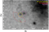 |
Fig. 4 PS1 source and background extraction region. |
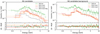 |
Fig. 5 Source (left) and background (right) spectra for the PS1 neutron star candidate. The TBabs*pow model is displayed on top of the source spectra. |
Best-fit results of the PS1 point source in the geometrical centre.
5 Conclusions
We investigated the recently discovered SNR G53.41+0.03 with a new dedicated XMM-Newton observation. Our main findings are as follows:
-
The X-ray morphology of the SNR is consistent with the detected radio structure in Driessen et al. (2018) and consists of an incomplete shell, with the southern part being either below the detection threshold or missing;
-
There are two unique regions of the remnant with significantly detected emission characterised by the NEI plasma model. The difference in their brightness and plasma characteristics is likely caused by the higher density in the brighter region and a combination of lower density and the proximity to the Galactic plane in the fainter region;
-
The spectral analysis reveals the age of the SNR to likely be in range 1000–5000 yr;
-
We find two point sources in the geometrical centre of the remnant, one of which we confirm as a YSO. The other point source has characteristics consistent with a magnetar, but further investigations are required to confirm its nature.
Acknowledgements
We would like to thank N.D. Degenaar, R.A.D. Wijnands for discussions on the topic of neutron stars, G. Mastroserio, R.M. Connors, J.V. Hernández Santisteban for advise on XSPEC’s MCMC and XMM helpdesk team for their technical support. We would also like to thank the anonymous referee for their comments that greatly improved this paper. The work of V.D. is supported by a grant from NWO graduate program/GRAPPA-PhD program. P.Z. acknowledges the support from the NWO Veni Fellowship, grant no. 639.041.647 and NSFC grant 11590781. L.N.D. acknowledges support from the European Research Council (ERC) under the European Union’s Horizon 2020 research and innovation programme (grant agreement no. 694745). This research made use of ASTROPY, a community-developed core PYTHON package for Astronomy (Astropy Collaboration 2013), MATPLOTLIB (Hunter 2007) and CORNER (Foreman-Mackey 2016). We further made use of SAOIMAGE DS9 (Joye & Mandel 2003), XSPEC (Arnaud 1996) and the SAO/NASA Astrophysics Data System.
Appendix A MCMC results for SNR regions 1, 2, and 3
 |
Fig. A.1 Two-dimensional correlation distributions of the TBabs*vnei part of the model for region 1 of the SNR G53.41+0.03. Posterior distributions of individualparameters are described by the median and the 1σ confidence interval. Contours in the two-dimensional histogram represent 0.5, 1, 1.5, and 2σ levels. Instrumental line components are not displayed for readability reasons. Full version of the figure, including the instrumental line components, is available in the zenodo archive. (https://doi.org/10.5281/zenodo.4737383) |
Appendix B MCMC results for the neutron star candidate PS1
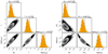 |
Fig. B.1 Two-dimensional correlation distributions of the TBabs*pow (left) and TBabs*bbodyrad (right) models for the PS1 neutron star candidate. Posteriordistributions of individual parameters are described by the median and the 1σ confidence interval. Contours in the two-dimensional histogram represent the 0.5, 1, 1.5, and 2σ levels. |
References
- Anderson, L. D., Wang, Y., Bihr, S., et al. 2017, A&A, 605, A58 [NASA ADS] [CrossRef] [EDP Sciences] [Google Scholar]
- Arnaud, K. A. 1996, in Astronomical Data Analysis Software and Systems V, 101, 17 [Google Scholar]
- Astropy Collaboration (Robitaille, T. P., et al.) 2013, A&A, 558, A33 [NASA ADS] [CrossRef] [EDP Sciences] [Google Scholar]
- Borkowski, K. J., Lyerly, W. J., & Reynolds, S. P. 2001, ApJ, 548, 820 [Google Scholar]
- Cash, W. 1979, ApJ, 228, 939 [Google Scholar]
- Condon, J. J., & Ransom, S. M. 2016, Essential Radio Astronomy (Princeton University Press), 376 [Google Scholar]
- Domcek, V., van den Eijnden, J., Escorial, A. R., et al. 2019, ATel, 13215, 1 [NASA ADS] [Google Scholar]
- Driessen, L. N., Domček, V., Vink, J., et al. 2018, ApJ, 860, 133 [Google Scholar]
- Ferrand, G., & Safi-Harb, S. 2012, Adv. Space Res., 49, 1313 [Google Scholar]
- Foreman-Mackey, D. 2016, J. Open Source Softw., 1, 24 [Google Scholar]
- Giardino, G., Favata, F., Micela, G., Sciortino, S., & Winston, E. 2007, A&A, 463, 275 [NASA ADS] [CrossRef] [EDP Sciences] [Google Scholar]
- Goodman, J., & Weare, J. 2010, Commun. Appl. Math. Comput. Sci., 5, 65 [Google Scholar]
- Gotthelf, E. V., Halpern, J. P., & Alford, J. 2013, ApJ, 765, 58 [Google Scholar]
- Green, D. A. 2019, JApA, 40, 36 [NASA ADS] [Google Scholar]
- Hunter, J. D. 2007, Comput. Sci. Eng., 9, 90 [NASA ADS] [CrossRef] [Google Scholar]
- Joye, W., & Mandel, E. 2003, in ASP Conf. Ser., 295, Astronomical Data Analysis Software and Systems XII, eds. H. Payne, R. Jedrzejewski, & R. Hook, 489 [Google Scholar]
- Kaastra, J. S., & Bleeker, J. A. M. 2016, A&A, 587, A151 [NASA ADS] [CrossRef] [EDP Sciences] [Google Scholar]
- Kaspi, V. M., Roberts, M. S. E., & Harding, A. K. 2006, in Compact stellar X-ray sources, 39 (Cambridge University Press), 279 [NASA ADS] [CrossRef] [Google Scholar]
- Kim, C. G. & Ostriker, E. C. 2015, ApJ, 802, 99 [NASA ADS] [CrossRef] [Google Scholar]
- Kim, H.-j., Koo, B.-c., & Davis, C. J. 2015, ApJ, 802, 59 [NASA ADS] [CrossRef] [Google Scholar]
- Koo, B.-C., Kim, C.-G., Park, S., & Ostriker, E. C. 2020, ApJ, 905, 35 [NASA ADS] [CrossRef] [Google Scholar]
- Kuntz, K. D., & Snowden, S. L. 2008, A&A, 478, 575 [NASA ADS] [CrossRef] [EDP Sciences] [Google Scholar]
- Masui, K., Mitsuda, K., Yamasaki, N. Y., et al. 2009, Publ. Astron. Soc. Jpn., 61, S115 [CrossRef] [Google Scholar]
- Merloni, A., Predehl, P., Becker, W., et al. 2012 ArXiv e-prints [arXiv:1209.3114] [Google Scholar]
- Meyer, D. M., Langer, N., Mackey, J., Velázquez, P. F., & Gusdorf, A. 2015, MNRAS, 450, 3080 [NASA ADS] [CrossRef] [Google Scholar]
- Olausen, S. A., & Kaspi, V. M. 2013, ApJS, 212, 6 [Google Scholar]
- Petre, R., Becker, C. M., & Winkler, P. F. 1996, ApJ, 465, L43 [NASA ADS] [CrossRef] [Google Scholar]
- Potekhin, A. Y., Zyuzin, D. A., Yakovlev, D. G., Beznogov, M. V., & Shibanov, Y. A. 2020, MNRAS, 496, 5052 [NASA ADS] [CrossRef] [Google Scholar]
- Predehl, P., & Schmitt, J. H. M. M. 1995, A&A, 500, 459 [Google Scholar]
- Reynolds, S. P. 2017, Dynamical Evolution and Radiative Processes of Supernova Remnants, eds. A. W. Alsabti, & P. Murdin (Cham: Springer International Publishing), 1981 [Google Scholar]
- Rodriguez, J., Tomsick, J. A., Bodaghee, A., et al. 2009, A&A, 508, 889 [NASA ADS] [CrossRef] [EDP Sciences] [Google Scholar]
- Sasaki, M., Plucinsky, P. P., Gaetz, T. J., et al. 2004, ApJ, 617, 322 [NASA ADS] [CrossRef] [Google Scholar]
- Shimwell, T. W., Röttgering, H. J. A., Best, P. N., et al. 2017, A&A, 598, A104 [NASA ADS] [CrossRef] [EDP Sciences] [Google Scholar]
- Sun, L., & Chen, Y. 2020, ApJ, 893, 90 [NASA ADS] [CrossRef] [Google Scholar]
- Vink, J. 2020, Physics and Evolution of Supernova Remnants, Astronomy and Astrophysics Library (Cham: Springer International Publishing) [CrossRef] [Google Scholar]
- Vink, J., Kaastra, J. S., & Bleeker, J. A. 1997, A&A, 328, 628 [NASA ADS] [Google Scholar]
- Vink, J., Broersen, S., Bykov, A., & Gabici, S. 2015, A&A, 579, A13 [NASA ADS] [CrossRef] [EDP Sciences] [Google Scholar]
- Weaver, R., McCray, R., Castor, J., Shapiro, P., & Moore, R. 1977, ApJ, 218, 377 [Google Scholar]
- Winston, E., Megeath, S. T., Wolk, S. J., et al. 2010, AJ, 140, 266 [NASA ADS] [CrossRef] [Google Scholar]
Driessen et al. (2018) had an incorrect  dependence due to a missed normalisation factor.
All Tables
Volume of emitting plasma, number density, and plasma age estimates for regions in SNR G53.41+0.03.
All Figures
|
Fig. 1 SNR G53.41+0.03 with a type I outburst of the high mass X-ray binary IGR J19294+1816 in October 2019. Left: grey-scale image in the energy range 0.8–4.0 keV. Radio contours of the THOR VGPS survey (Anderson et al. 2017) with levels –(0.013, 0.01475, 0.02) Jy beam−1 are overlaid on top of the X-ray data. Right: three-colour image (red 0.8–1.5 keV, green 1.5–2.5 keV, and blue 2.5–4.0 keV) of the extraction and exclusion regions used in the analysis. We applied square-root scaling to the left image and logarithmic scaling to the right image to improve visibility. |
| In the text | |
|
Fig. 2 Best-fit models for the source and the background region spectra. A black dashed line shows the MOS 2 detector background model for individual regions. In region 2 we display the best-fit model fitted in the 0.5–5.0 keV energy range. |
| In the text | |
|
Fig. 3 Two-dimensional contour plots of emission measure vs. ionisation age, τ. Dashed linesrepresent curves of the same (τ∕ne) prescribed by Eq. (5). |
| In the text | |
|
Fig. 4 PS1 source and background extraction region. |
| In the text | |
|
Fig. 5 Source (left) and background (right) spectra for the PS1 neutron star candidate. The TBabs*pow model is displayed on top of the source spectra. |
| In the text | |
|
Fig. A.1 Two-dimensional correlation distributions of the TBabs*vnei part of the model for region 1 of the SNR G53.41+0.03. Posterior distributions of individualparameters are described by the median and the 1σ confidence interval. Contours in the two-dimensional histogram represent 0.5, 1, 1.5, and 2σ levels. Instrumental line components are not displayed for readability reasons. Full version of the figure, including the instrumental line components, is available in the zenodo archive. (https://doi.org/10.5281/zenodo.4737383) |
| In the text | |
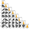 |
Fig. A.3 Same as in Fig. A.1 but for model TBabs*vnei (5keV cut) for region 2. |
| In the text | |
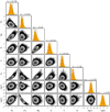 |
Fig. A.2 Same as in Fig. A.1 but for model TBabs*vnei for region 2. |
| In the text | |
|
Fig. B.1 Two-dimensional correlation distributions of the TBabs*pow (left) and TBabs*bbodyrad (right) models for the PS1 neutron star candidate. Posteriordistributions of individual parameters are described by the median and the 1σ confidence interval. Contours in the two-dimensional histogram represent the 0.5, 1, 1.5, and 2σ levels. |
| In the text | |
Current usage metrics show cumulative count of Article Views (full-text article views including HTML views, PDF and ePub downloads, according to the available data) and Abstracts Views on Vision4Press platform.
Data correspond to usage on the plateform after 2015. The current usage metrics is available 48-96 hours after online publication and is updated daily on week days.
Initial download of the metrics may take a while.