| Issue |
A&A
Volume 658, February 2022
|
|
|---|---|---|
| Article Number | A29 | |
| Number of page(s) | 13 | |
| Section | Stellar structure and evolution | |
| DOI | https://doi.org/10.1051/0004-6361/202142441 | |
| Published online | 27 January 2022 | |
The iron and oxygen content of LMC Classical Cepheids and its implications for the extragalactic distance scale and Hubble constant
Equivalent width analysis with Kurucz stellar atmosphere models⋆,⋆⋆
1
European Southern Observatory, Karl-Schwarzschild-Strasse 2, 85478 Garching bei München, Germany
e-mail: This email address is being protected from spambots. You need JavaScript enabled to view it.
2
Space Telescope Science Institute, 3700 San Martin Drive, Baltimore, MD 21218, USA
3
Department of Physics and Astronomy, Johns Hopkins University, Baltimore, MD 21218, USA
4
Institute of Physics, Laboratory of Astrophysics, École Polytechnique Féderale del Lausanne (EPFL), Observatoire de Suverny, 1290 Versoix, Switzerland
5
LMU München, Universitätssternwarte, Scheinerstrasse 1, München 81679, Germany
6
Institute for Astronomy, University of Hawaii at Manoa, 2680 Woodlawn Drive, Honolulu, HI 96822, USA
7
Mitchell Institute for Fundamental Physics and Astronomy, Department of Physics and Astronomy, Texas A&M University, College Station, TX 77843, USA
8
Dipartimento di Fisica e Astronomia Augusto Righi, Università degli Studi di Bologna, Via Gobetti 93/2, 40129 Bologna, Italy
9
INAF – Osservatorio di Astrofisica e Scienza dello Spazio di Bologna, Via Gobetti 93/3, 40129 Bologna, Italy
Received:
14
October
2021
Accepted:
8
November
2021
Abstract
Context. Classical Cepheids are primary distance indicators and a crucial stepping stone in determining the present-day value of the Hubble constant H0 to the precision and accuracy required to constrain apparent deviations from the ΛCDM Concordance Cosmological Model.
Aims. We measured the iron and oxygen abundances of a statistically significant sample of 89 Cepheids in the Large Magellanic Cloud (LMC), one of the anchors of the local distance scale, quadrupling the prior sample and including 68 of the 70 Cepheids used to constrain H0 by the SH0ES program. The goal is to constrain the extent to which the luminosity of Cepheids is influenced by their chemical composition, which is an important contributor to the uncertainty on the determination of the Hubble constant itself and a critical factor in the internal consistency of the distance ladder.
Methods. We derived stellar parameters and chemical abundances from a self-consistent spectroscopic analysis based on equivalent width of absorption lines.
Results. The iron distribution of Cepheids in the LMC can be very accurately described by a single Gaussian with a mean [Fe/H] = −0.409 ± 0.003 dex and σ = 0.076 ± 0.003 dex. We estimate a systematic uncertainty on the absolute mean values of 0.1 dex. The width of the distribution is fully compatible with the measurement error and supports the low dispersion of 0.069 mag seen in the near-infrared Hubble Space Telescope LMC period–luminosity relation. The uniformity of the abundance has the important consequence that the LMC Cepheids alone cannot provide any meaningful constraint on the dependence of the Cepheid period–luminosity relation on chemical composition at any wavelength. This revises a prior claim based on a small sample of 22 LMC Cepheids that there was little dependence (or uncertainty) between composition and near-infrared luminosity, a conclusion which would produce an apparent conflict between anchors of the distance ladder with different mean abundance. The chemical homogeneity of the LMC Cepheid population makes it an ideal environment in which to calibrate the metallicity dependence between the more metal-poor Small Magellanic Cloud and metal-rich Milky Way and NGC 4258.
Key words: techniques: spectroscopic / stars: variables: Cepheids / Magellanic Clouds / dark energy / distance scale
Full Tables 1–8 and Appendix B are only available at the CDS via anonymous ftp to cdsarc.u-strasbg.fr (130.79.128.5) or via http://cdsarc.u-strasbg.fr/viz-bin/cat/J/A+A/658/A29
Based on observations collected at the European Southern Observatory under ESO programmes 66.D-0571 and 106.21ML.003.
© ESO 2022
1. Introduction
The current discrepancy regarding the present-day value of the Hubble constant H0 is arguably one of the most far-reaching open problems in astrophysics today. The extrapolation of early-Universe cosmic microwave background measurements assuming the Λ cold dark matter (CDM) Cosmological Concordance Model predicts a value of H0 = 67.4 ± 0.5 km s−1 Mpc−1 (Planck Collaboration VI 2020). Comparison to the best late-Universe local measurement of H0 = 73.2 ± 1.3 km s−1 Mpc−1 (Riess et al. 2021, SH0ES project), which is independent of any such assumptions, reveals a significant 4.2σ tension. Moreover, all recent local determinations, obtained by different groups with different methods, exceed the early-Universe prediction (e.g., Verde et al. 2019; Riess 2020, and references therein). The conclusion that there is indeed a meaningful difference between early- and local-Universe values of H0 is therefore by now almost inescapable. This is hugely consequential: in spite of its many phenomenological successes, the ΛCDM model does not provide a complete description of the Universe.
Classical Cepheids play a pivotal role in this context, because they are primary distance indicators and a crucial stepping stone in determining the present-day value of the Hubble constant to the precision and accuracy required to constrain possible deviations from ΛCDM. In particular, the SH0ES project has built a clean, three-rung distance ladder based on them and on type-Ia supernovæ. Their goal is to measure the local value of the Hubble constant H0 to an accuracy of better than 1% so as to provide a meaningful match to the early-Universe value derived from the cosmic microwave background.
Cepheids can be used to measure distances because their brightness changes periodically with time according to the Leavitt Law (Leavitt & Pickering 1912), which links the period of such pulsations, which is independent of distance, to their mean magnitude, which scales as the inverse of the distance squared (period–luminosity (PL) relation). The uncertainty on the behaviour of the PL relation with chemical composition is a major contributor to the overall SH0ES H0 error budget (0.9% out of 1.8%, Riess et al. 2021). Indeed, recent results using Galactic and Magellanic Cloud Cepheids confirm that, while progress is being made in terms of sample sizes, as crucially enabled by Gaia parallaxes, the slope of a potential dependence of the Cepheid luminosity on metal content remains too loosely constrained, with significant differences between different studies; for example −0.221 ± 0.051 mag dex−1 (Breuval et al. 2021, see also Gieren et al. 2018) versus −0.456 ± 0.099 mag dex−1Ripepi et al. (2021) for the slope in the Ks band.
Here, we provide accurate direct abundance measurements from high-resolution spectroscopy of Cepheids stars in the Large Magellanic Cloud (LMC), one of the three anchor galaxies in the SH0ES distance ladder (Riess et al. 2019). The paper is organised as follows. In Sect. 2 we present the data and their reduction to calibrated one-dimensional spectra. Section 3 describes the derivation of the stellar parameters that are needed in order to measure chemical abundances. These are discussed in Sects. 4 and 5 for iron and oxygen, respectively. Finally, conclusions are drawn in Sect. 6.
2. Observations and data reduction
We assembled our sample of 89 Classical Cepheids in the LMC by combining proprietary data for 67 out of the 70 stars that define the SH0ES fiducial PL relation (Riess et al. 2019) with 22 archival spectra observed in the same instrumental setup. For the mentioned sample of 67 stars, this is the first measurement of their chemical composition. Iron abundances for the other ones were published by Romaniello et al. (2008, OGLE510/HV879 is in common between the two samples and is considered here only once; see Table 1). Here, we revise those measurements, which we find were affected by undetected systematic errors.
Log of the spectroscopic observations of the 68 SH0ES Cepheids.
All of the stars are listed in the OGLE IV catalogue (Udalski et al. 2015; Soszyński et al. 2015). In the following, we use their OGLE identifier, which we shortened for convenience (e.g., OGLE-LMC-CEP-0966 to OGLE0966). Their on-sky distribution and the PL relations in the various bands of the SH0ES sample are presented in Figs. 1 and 2, respectively.
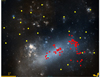 |
Fig. 1. Distribution on the plane of the sky of the 68 SH0ES Classical Cepheids targeted in this paper (red dots). The two stars for which we do not have spectroscopic data are marked in cyan. The stars from the Romaniello et al. (2008) sample that we re-analyse here are shown as yellow dots. The figure was generated with the ‘Aladin sky atlas’ software (Boch & Fernique 2014) using a DSS2 colour image of the LMC as background. |
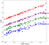 |
Fig. 2. PL relations in the various bands of the sky of the SH0ES Classical Cepheids (Riess et al. 2019, see Table 2 and Fig. 3). The two for which we do not have spectroscopic data are marked as open circles. The scatter in the |

We have excluded two of the SH0ES stars from our spectroscopic sample (OGLE1940, OGLE1945; open circles in Fig. 2) because they are too faint in the optical to obtain spectra in a reasonable amount of time. They are also significant outliers from the PL relation in all magnitudes except  and excluding them from the analysis has no impact on our conclusions.
All 89 stars were observed with the UVES spectrograph at the ESO VLT telescope in the UVES 580 setting. This spectrograph covers the wavelength range between 4780 and 6800 Å with a gap between 5760 and 5830 Å. The instrumental resolving power is R ∼ 50 000, but Cepheids have intrinsically broad spectral lines, yielding an effective value of R ∼ 20 000. The proprietary observations of the SH0ES sample were carried out in Service Mode. Observing constraints and exposure times were adapted to each star in order to deliver data of uniform quality (signal-to-noise ratios higher than 40). No constraints were set on the pulsational phase at the time of observation, which is therefore random. In two cases (OGLE0545, OGLE1647), observations were at first executed outside of the constraints we had specified. They were subsequently successfully repeated and we did not use the first set of data, because they did not add significantly to the final quality. The log of the observations we did use in the analysis is reported in Table 1. We refer the reader to Romaniello et al. (2008) for the details of the observations of the archival Cepheids.
We downloaded the raw science files from the ESO Science Archive1 both for our proprietary data and the archival ones, together with the calibrations provided by the system according to the instrument Calibration Plan (Sbordone & Ledoux 2020). We reduced the data with the instrument pipeline version 6.1.3 (Møller Larsen et al. 2020), executed within the ESOReflex environment (Freudling et al. 2013), and added a custom step to the default processing cascade to combine repeated observations of the same targets. In all cases, these are taken in sequence (see Table 1), so a simple co-addition of the raw 2D frames is sufficient.
In the first pass, all data were processed with the default pipeline recipe parameters, which were then optimised by individually inspecting the results. In all cases, we reduced the rejection threshold during spectral extraction from 10 to 5σ (parameter reduce.extract.kappa in the uves_obs_scired recipe) to limit the impact of cosmic ray hits and detector defects. Visual inspection of the results confirmed that no significant residuals are present. In the case of star OGLE0936, the trace of a bright neighbouring star is clearly visible in the 2D spectrum and the default extraction window includes them both. We therefore tailored the window to only include the star of interest (parameter reduce.extract.kappa = 26 in the uves_obs_scired recipe). In all other cases, the default recipe parameters were confirmed to be adequate and were left unchanged.
3. Stellar parameters
3.1. The equivalent width method
In order to self-consistently determine the stellar parameters (effective temperature Teff, surface gravity in logarithmic units log(g) and microturbulent velocity vturb) and chemical abundances, we use the equivalent width (EW) method. Very briefly, for each star, the EWs of iron lines as measured in the observed spectrum are compared to the ones from a stellar atmosphere model for a given set of stellar parameters to derive the abundances from each individual line. These are then iterated upon until convergence is reached when the following conditions are met:
– Effective temperature is derived by imposing excitation equilibrium, that is, by imposing that there be no residual correlation between the iron abundance and the excitation potential χ of the neutral iron lines. As demonstrated by Mucciarelli & Bonifacio (2020) for example, above a metallicity of ∼ − 1.5, spectroscopic temperatures provide an unbiased estimate.
– The best value of surface gravity comes from imposing ionisation equilibrium, thus requiring that, for a given species, the abundance is the same within the uncertainties from lines of two different ionisation states (in our case, neutral and singly ionised iron lines).
– Microturbulent velocity is set by requiring that there be no residual correlation between the iron abundance and the line EW as a measure of the line strength.
– The final iron abundance is the mean of the iron abundances from the individual lines in the convergence iteration.
– The initial values of the parameters were set for all stars as follows: Teff = 5500 K, log(g) = 1 cm s−2, [Fe/H] = −0.33 dex and vturb = 2.50 km s−1. Changing each of them by up to a factor of two influences the resulting abundances randomly at the level of a few hundredths of a dex.
– The abundance of oxygen is then measured with the stellar parameters determined as described above.
We used the list provided by Genovali et al. (2013) as input for the spectral location of unblended FeI and FeII lines (Table 2); it was compiled specifically for Cepheid stars, thus providing a clean set of lines to avoid line crowding as much as possible for these types of stars, which have intrinsically broad features (FWHM ∼ 0.2 − 0.3 Å). We measured the EWs with the DAOSPEC code (Stetson & Pancino 2008), which was executed on our entire sample of stars using the 4DAO software (Mucciarelli 2013).
189 FeI, 28 FeII, and 2 OI lines used as input in the analysis.
In our analysis, we adopted the GALA implementation of the EW method, which was extensively and specifically tested on UVES data (Mucciarelli et al. 2013). As input physics, we used the classical grid of ATLAS9 Local Thermodynamical Equilibrium (LTE) stellar atmosphere models (Castelli & Kurucz 2004). During the analysis, for each spectrum, lines are rejected from the fit based on a number of quality criteria, so that the final set of lines used in the analysis varies from one spectrum to another, depending on circumstances, such as signal-to-noise ratio and line depth. However, in all cases, a sufficient number of lines are retained such that the resulting solution is meaningful in terms of stellar parameters and elemental abundances. This is shown in Fig. 3, where the number of iron lines used in the analysis for each spectrum is given.
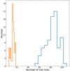 |
Fig. 3. Number of FeI (blue histogram) and FeII (orange histogram) spectral lines retained in the abundance analysis of each of the 89 programme stars after outlier rejection as part of the fitting procedure with the GALA code (see Sect. 3.1). The full input line list is reported in Table 2. |
Once convergence is reached, the uncertainty on the elemental abundance is computed, taking into account the covariance among the stellar parameters according to the prescription of Cayrel et al. (2004).
In order to gauge the quality of the results, in Fig. 4 we plot the distributions of the quantities that are minimised when computing the stellar parameters: the slope Sχ of FeI abundance versus excitation potential χ for Teff, the slope SEWR of the relation between FeI abundance and reduced EW (EWR) = log(EW/λ) for vturb, and the difference between FeI and FeII for log(g). In order to interpret the residuals in the convergence criteria in terms of their impact on the final abundance determination, which is our ultimate goal, in panels a and b of the same figure we also plot the corresponding peak-to-peak values of the spread in iron abundance, computed for every star as:
 (1)
(1)
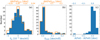 |
Fig. 4. Histograms of the output values of the diagnostics used to derive the stellar parameters for the 89 stars in our combined sample. Panel a: slope Sχ of FeI abundance vs. excitation potential χ used to derive the effective temperature Teff (solid blue curve, bottom x scale). The corresponding peak-to-peak values of the spread in iron abundance (ΔA(FeI)p2p, see Eq. (1)) are plotted as an open orange curve (top x scale). Panel b: slope SEWR of the relation between FeI abundance and reduced EW EWR = log(EW/λ), which ranges between −5.5 and −4.5, and is used to constrain the microturbulent velocity vturb (solid blue curve, bottom x scale). Also here, the corresponding peak-to-peak values of the spread in iron abundance (ΔA(FeI)p2p, see Eq. (1)) are plotted as an open orange curve (top x scale). Panel c: difference between FeI and FeII, the minimisation of which is used to determine the surface gravity log(g). The mean and standard deviation of the distribution are 0.007 and 0.033 dex, respectively, indicating excellent agreement between the derived FeI and FeII abundances, and hence gravity, with no appreciable systematic errors. |
where S = Sχ or SEWR and l is the lever range spanned in χ and EWR, respectively, by the lines ultimately used in the fit. In other words, these peak-to-peak values are the maximum scatter in the abundance introduced by residual correlations in the minimisation process. As it can be seen, their impact is of the order of a mere few hundredths of a dex at maximum. The same applies when considering the iron abundances of the 89 stars versus the stellar parameters that, as shown in Fig. 5, do not show any appreciable residual trend (the expectation being that the chemical composition of a Cepheid does not depend on its stellar parameters along its crossings of the instability strip). The derived stellar parameters are reported in Table 3 for the SH0ES sample and in Table 4 for the archival one. In order to make our analysis reproducible, in Appendices A and B we provide, respectively, the full GALA configuration file we have used and the EWs of the individual lines for each star.
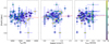 |
Fig. 5. Measured iron abundance vs. stellar parameters simultaneously derived in the GALA analysis. As expected, hardly any residual trend is present (red line). The points are colour-coded according to the phase along the pulsational cycle within which the stars were observed, with the scale represented by the bar on the far right. |
Stellar parameters as derived in the abundance analysis for the SH0ES sample.
Stellar parameters as re-derived here in the abundance analysis for the Romaniello et al. (2008) archival sample.
3.2. Stellar versus pulsational parameters
The fact that Cepheids pulsate according to well-defined laws allows us to perform additional consistency checks on the stellar parameters derived in the abundance analysis. To this end, in Fig. 6 we plot them as a function of pulsational period. As can be seen, the iron abundance shows a negligible correlation with the period, as expected from it being an intrinsic property of the star independent from the pulsation mechanism. On the other hand, correlations are found between the stellar parameters. This is also expected, in that they reflect the location of the stars in the instability strip when they were observed. The scatter is dominated by having caught the stars at a random phase along the pulsational cycle.
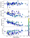 |
Fig. 6. Stellar parameters as measured in our analysis vs the pulsational periods of the stars. The iron abundance shows a negligible correlation with the period, further confirming the robustness of our analysis. On the other hand, for the other stellar parameters, the correlations reflect the location of the instability strip, with a scatter dominated by having observed the stars at a random phase in the pulsational cycle. The points are colour-coded according to the phase along the pulsational cycle within which the stars were observed, with the scale represented by the bar on the far right. |
Figure 7 displays the correlation of temperature with the phase along the pulsation cycle within which each star was observed. As expected, the stars are coldest towards the middle of the pulsation cycle and get hotter at either extreme, with an excursion of about 1000 K. All of these diagnostics further confirm the soundness and robustness of our analysis.
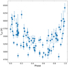 |
Fig. 7. Derived stellar effective temperature (Teff) as a function of the phase along the pulsational cycle within which each star was observed (see Table 3). The size of the mean error on Teff is shown by the error bar in the lower-left corner. |
4. Iron abundances
Because of the large number of available lines in the optical spectral region, iron is often used as as a proxy for the overall metal content and as a reference against which other elemental abundances are measured. The FeI and FeII abundances derived from the procedure described above are listed in Tables 5 and 6 for the SH0ES and archival sample, respectively. In the following, unless otherwise noted, we refer to FeI simply as iron when talking about abundances.
Stellar iron abundances for the SH0ES sample.
Stellar iron abundances from the re-analysis of the Romaniello et al. (2008) archival sample.
In Fig. 8, we show the histogram of the iron values for our 89 stars; fitting it with a Gaussian yields a mean value of −0.409 ± 0.003 dex, with a width σ = 0.076 ± 0.003 dex (the values of straight mean and standard deviation are −0.41 and 0.09, respectively). The latter is almost indistinguishable from the mean error as propagated through the abundance analysis (∼0.07 dex, green dashed vertical lines), making the distribution consistent with a single abundance as broadened by the observational uncertainties. The uncertainty on the mean value quoted above is the random one determined by the internal consistency of our method, the intrinsic width of the distribution and the number of stars in our sample. We estimate the systematic component to be 0.1 dex (see Sect. 4.1 below). This systematic uncertainty only affects the absolute mean value of the distribution, but not its width.
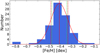 |
Fig. 8. Histogram of the iron abundances measured for the combined sample of 89 LMC Cepheids, together with its best fitting Gaussian (solid red curve). The vertical lines mark the position of the peak of the Gaussian ([Fe/H] = −0.409 ± 0.003, solid red), plus and minus one Gaussian sigma (σ = 0.076 ± 0.003, red dashed) and the mean of the error on the iron abundance resulting from the spectral analysis (∼0.07 dex, green dashed line, Tables 5 and 6). |
4.1. Comparison with previous results
The most direct comparison with our results is with those presented by Romaniello et al. (2008). The main difference between the analyses is that here we derive the stellar effective temperature together with the other parameters (see Sect. 3.1), while Romaniello et al. (2008) first fix the temperature using the Line Depth Ratio (LDR; specifically in the implementation of Kovtyukh & Gorlova 2000) method, and then derive the remaining parameters log(g) and vturb, and the iron abundance.
In the left panel of Fig. 9, we plot the histogram of the iron abundances from Table 9 of Romaniello et al. (2008), together with a Gaussian fit to it. The mean value of the distribution is −0.30 ± 0.02 dex with σ = 0.13 ± 0.02 dex, to be compared to −0.409 and 0.076 dex, respectively, for our 89 stars (see Sect. 4 above).
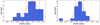 |
Fig. 9. Histograms of the iron abundance distributions of the sample of the 22 Cepheids in the Romaniello et al. (2008) sample. Left panel: original values from Romaniello et al. (2008, see their Table 9), together with the best fitting Gaussian (solid red curve). The vertical lines mark the position of the peak of the Gaussian (solid red) and plus and minus one Gaussian sigma (red dashed). Right panel: same as the left panel, but for our re-analysis of the same spectra. The distribution in the left panel was artificially broadened because of a spurious trend in [Fe/H] vs. vturb resulting from the abundance analysis (see Fig. 10 and the text). |
The results of the present analysis on the Romaniello et al. (2008) sample are shown in the right panel of Fig. 9. With a measured Gaussian mean of −0.43 ± 0.01 and σ = 0.08 ± 0.01 dex, the ensemble properties of the reanalysed Romaniello et al. (2008) sample compare very well with those of the 89 stars of the combined sample, as well as with those of the 68 SH0ES stars alone (mean = −0.399 ± 0.003 dex, σ = 0.072 ± 0.003 dex). This rules out differences between the samples and points to differences in the abundance analysis instead.
The discrepancy in the mean iron abundance between the one we derive here and the one in Romaniello et al. (2008) can be traced back to an offset of about 170 K in the temperatures as computed with the two methods, the present re-analysis yielding the lower values. The observed difference in iron is then consistent with the expectation that an increase in temperature of 100 K at fixed vturb and log(g) results in an increase in [Fe/H] of about 0.07 dex (Romaniello et al. 2008).
As for the difference in dispersion, it can be explained by the fact that the analysis by Romaniello et al. (2008) leaves a significant residual slope between iron abundance and stellar microturbulent velocity (see Fig. 10). Once this is removed, for example with a simple linear regression, the remaining scatter is fully compatible with the quoted uncertainty in their measured iron abundances of ‘typically 0.08–0.1 dex’. Furthermore, in the re-analysis of the spectra, there are no significant residual trends (see Fig. 5), as is the case for the whole sample. We therefore confirm that the observed spread in iron abundances among the stars is fully compatible with a measurement uncertainty of ∼0.08 dex, without additional sources of broadening.
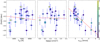 |
Fig. 10. Measured iron abundance vs. stellar parameters as derived in Romaniello et al. (2008, see their Table 9), together with the results of a linear regression (red lines). A clear residual trend is present with vturb, which is responsible for the large scatter of σ = 0.13 that our analysis does not confirm. The points are colour-coded according to the phase along the pulsational cycle within which the stars were observed, with the scale represented by the bar on the far right. |
Finally, we note that our results compare very well with those in Urbaneja et al. (2017), who found a mean abundance of [Fe/H] = −0.34 ± 0.11 for 23 LMC blue supergiant stars. These stars are a different from Cepheids but the two types are coeval; they were analysed with a method that is completely independent of the one we use here, also incorporating non-LTE effects. The remarkable agreement in iron content between the two samples indicates that the effects of systematic errors in our analysis, including from possible departures from LTE, are smaller than 0.1 dex.
4.2. Implications for the PL relation and the distance scale
The 89 LMC Cepheids we analyse here were not selected in any particular way with respect to their iron content, which was not known at all before their spectra were taken. The fact they do not show any appreciable deviation from a Gaussian with a width dictated by the rather stringent measurement uncertainty of ∼0.07 dex (see Fig. 8), together with the fact that they are distributed over the full extent of the LMC (see Fig. 1), is indicative that it is a general property of the LMC Cepheids as a population to have the same iron abundance within that limit.
The iron content therefore does not add to the scatter of the LMC PL relation, which is advantageous when used as a tool to measure distances. On the other hand, this also means that Cepheids in the LMC alone cannot be used to determine the extent to which the relation itself depends on the chemical composition, the uncertainty on which is an important contributor to the total error budget when determining H0 (0.9% out of 1.8%, Riess et al. 2021). This is illustrated in the right panel of Fig. 11, where it is apparent that the span of iron abundances is too small with respect to the size of the measurement errors to determine any meaningful dependence on the magnitude residuals in the H band with respect to the fiducial PL relation of Riess et al. (2019). For comparison, we show a line for no dependence and a ∼ − 0.2 mag dex−1 dependence as found by other measurements from gradients within spiral galaxies or between galaxies with difference abundances (e.g., Riess et al. 2019; Breuval et al. 2021; Ripepi et al. 2021). Because of the large uncertainties on both axes, any attempt to measure a dependence from this data must take care to include both in a fit. This is inherently method-dependent for the reason that it is not well-constrained by the data and we quote illustrative results from two approaches, γ = −0.68 ± 0.34 with the fitexy algorithm described in Press & Teukolsky (1992), and −0.11 ± 1.3 from a non-linear least-squares from a Monte-Carlo Markov chain (lmfit).
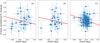 |
Fig. 11. Residuals in the H-band dereddened magnitude PL relation as a function of iron abundance. Panel a: original Romaniello et al. (2008) sample of 22 LMC Cepheids, with photometry from Persson et al. (2004). Panel b: same sample, but with the iron abundances as revised here. Panel c: SH0ES sample of 68 LMC Cepheids, with iron abundances as measured here and photometry from Riess et al. (2019). To guide the eye, in all panels, the red line indicates a metallicity dependence of the Cepheid PL of γ = −0.2 mag dex−1, which is often quoted in the recent literature (e.g., Riess et al. 2019; Breuval et al. 2021; Ripepi et al. 2021). |
We also revisit whether γ may be derived from the original Romaniello et al. (2008) sample of 22 LMC Cepheids and their revised values here as shown in Fig. 11 with important consequences for the determination of H0. It is apparent from Fig. 11 that the measurement errors in both axes from the earlier, smaller sample are too large (and the span of [Fe/H] too small) to usefully constrain γ, with even the more optimistic fitexy algorithm giving σγ > 0.4 mag dex−1 for either sample. We cannot reproduce the results of a very strong constraint of a minimal dependence of γ = 0.05 ± 0.02 for the H-band and γ = 0.02 ± 0.03 for the K-band given by Freedman & Madore (2011) from the original Romaniello et al. (2008) sample which would be more than 20 times better than what we find achievable. Not only is a small value and uncertainty in γ not supported by the small range of [Fe/H] within the LMC, but these low values and uncertainties are also inconsistent with the value of ∼ − 0.22 ± 0.05 mag dex−1 dependence in this region of the NIR found by Breuval et al. (2021) for example by comparing Cepheids between the LMC, Small Magellanic Cloud (SMC), and Milky Way to their geometric distances. Other hosts with a broader range of [Fe/H] can be used to measure γ internally. This is even possible within the MW using Gaia Early Data Release 3 (EDR3) Cepheid parallaxes, where Riess et al. (2021) found γ = −0.20 ± 0.12. While comparing hosts with different mean abundance and independent geometric distances reveals a significant metallicity dependence, setting γ = 0 would likewise cause the appearance of tension between the geometric anchors with different mean abundances as claimed by Efstathiou (2020)2. Therefore, the inability to constrain γ within the LMC Cepheid sample alone is an important conclusion in the context of determining the value of H0.
Such a narrow distribution in iron content across the surface of the LMC also implies that virtually no chemical enrichment took place in the look-back time covered by our sample. In order to quantify this, we converted the Cepheid pulsational periods into stellar evolutionary ages according to the relations by De Somma et al. (2021). The resulting distributions are shown in Fig. 12 for two assumptions about the amount of core convective overshooting during the core H-burning stage. Either way, the time-span is of the order of 50 Myr.
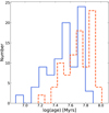 |
Fig. 12. Age distribution of our programme stars derived by applying the period–age relations by De Somma et al. (2021) for two assumptions on the amount of core convective overshooting during the core H-burning stage: no extension above the canonical value predicted by the Schwarzschild criterion (canonical scenario, solid blue line), or a moderate core overshoot (non-canonical scenario, dashed red line). |
5. Oxygen abundances
Oxygen is the third most abundant element in the Universe after hydrogen and helium, and the most abundant one among those not created in the Big Bang. It is also fairly easy to detect and measure as strong emission lines in HII regions in galaxies along the SH0ES distance ladder to H0 and is therefore often used as proxy for the global metallicity (e.g., Riess et al. 2016). However, gas-phase measurements are only a proxy for the stellar ones and may not give consistent results (e.g., Kewley & Ellison 2008; Davies et al. 2017). It is therefore important to provide direct measurements on the Cepheids themselves.
However, our instrumental setup includes only very few oxygen lines from which to measure the abundance, which makes the determination rather more uncertain than that of iron. Specifically, we used the two forbidden [OI] lines at 6300.30 and 6363.77 Å to measure the oxygen abundances for our stars. Both transitions cause strong airglow emissions in the night sky. However, at the spectral resolution of UVES, the heliocentric velocity at the time of observations and the radial velocity of the LMC of about 250 km s−1 shifts them sufficiently away from their rest-frame position so that the measurement is not affected by residuals in the sky subtraction.
The results are listed in Tables 7 and 8. For 29 out of 89 stars, we could not measure a meaningful oxygen abundance, either because the EW of the lines could not be measured, or because convergence was not reached in deriving the abundance.
Stellar oxygen abundances for the SH0ES sample.
Stellar oxygen abundances from the re-analysis of the Romaniello et al. (2008) archival sample.
The distribution of the measured oxygen abundances is shown in Fig. 13. The mean value from a Gaussian fit is [O/H] = −0.32 ± 0.01 dex with a width of σ = 0.09 ± 0.01 dex, which is consistent with the mean measurement error of 0.1 dex. Therefore, the same consideration of Sect. 4.2 on the unsuitability of LMC Cepheids alone to constrain the dependence of the PL relation on iron content applies to oxygen as well.
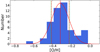 |
Fig. 13. Histogram of the oxygen abundances measured for the 60 out of 89 LMC Cepheids (see Table 7), together with its best fitting Gaussian (solid red curve). The vertical lines mark the position of the peak of the Gaussian (solid red), plus and minus one Gaussian sigma (red dashed) and the mean of the error on the iron abundance resulting from the spectral analysis (green dashed, Table 7). |
6. Summary and conclusions
In this study, we analysed the spectra of 89 LMC Cepheids to measure their iron and oxygen abundances. This is of crucial relevance for the local distance scale, of which the LMC is one of the anchors.
Our analysis indicates that the iron distribution of Cepheids in the LMC can be very accurately described by a single Gaussian with mean [Fe/H] = −0.409 ± 0.003 dex and σ = 0.076 ± 0.003 dex for iron and [O/H] = −0.32 ± 0.01 dex with a width of σ = 0.09 ± 0.01 dex for oxygen. We estimate a systematic uncertainty on the absolute mean values of 0.1 dex. In both cases, the observed scatter is fully compatible with the measurement error. Going beyond the present accuracy in order to characterise the chemical properties of LMC Cepheids will require a very significant effort and may not be worthwhile.
Our findings do not support the earlier results by Romaniello et al. (2008), who found a significantly larger distribution in iron (σ = 0.13 ± 0.02 dex). The difference can be explained by a residual spurious trend of the iron abundance versus the microturbulent velocity in their analysis. The difference of 0.1 dex in the mean values of iron can be explained by the different temperature scales. Here we derive the temperatures simultaneously with the other stellar parameters and abundances, while Romaniello et al. (2008) compute them a priori with the Line Depth Ratio method, also on the spectra themselves.
The fact that the chemical abundance distribution is effectively unresolved given the observational uncertainties that are attainable in practice implies that the LMC alone cannot be used to constrain the possible dependency of the Cepheid luminosity on their chemical composition, which is a source of major uncertainty in measuring the Hubble constant to ∼1%, as required to constrain possible deviations from the ΛCDM Cosmological Concordance Model. The most promising way to do so seems to be to combine the LMC with the SMC and the Galaxy, so as to achieve a long enough baseline in abundance with respect to the typical uncertainties.
On the other hand, the extreme chemical homogeneity of the LMC Cepheid population makes it an ideal environment in which to calibrate the PL relation at this particular metallicity. In retrospect, a crucial factor in the finding by the SH0ES team was that the period–Wesenheit relation in the HST-WFC3 H, V, and I bands has a very low intrinsic scatter of a mere 0.069 mag, or 3% (Riess et al. 2019).
Though Efstathiou (2020) noted that the discrepancy could be due to a metallicity dependence of the PL relation, which appears likely.
Acknowledgments
We warmly thank ESO’s Observing Programme Office and User Support Department for adapting the scheduling of our observations to the evolving constraints dictated by the Covid-19 pandemic. The outstanding job of the staff of ESO’s Paranal Science Operations in carrying out the observations under the gruelling circumstances is gratefully acknowledged. We thank Giulia De Somma, Marcella Marconi and Vincenzo Ripepi for fruitful discussions. We are grateful to the anonymous referee for carefully reading the manuscript and providing useful suggestions to improve it. S. M. and R. P. K. acknowledge support by the Munich Excellence Cluster Origins funded by the Deutsche Forschungsgemeinschaft (DFG, German Research Foundation) under Germany’s Excellence Strategy EXC-2094 390783311. R. I. A. acknowledges support from the Swiss National Science Foundation (SNSF) through an Eccellenza Professorial Fellowship (award PCEFP2_194638) as well as from the European Research Council (ERC) under the European Union’s Horizon 2020 research and innovation programme (Grant Agreement No. 947660). This research has made use of “Aladin sky atlas” developed at CDS, Strasbourg Observatory, France.
References
- Asplund, M., Grevesse, N., Sauval, A. J., et al. 2009, ARA&A, 47, 481 [Google Scholar]
- Barklem, P. S., Piskunov, N., & O’Mara, B. J. 2000, A&AS, 142, 467 [NASA ADS] [CrossRef] [EDP Sciences] [Google Scholar]
- Boch, T., & Fernique, P. 2014, Astronomical Data Analysis Software and Systems XXIII, 485, 277 [NASA ADS] [Google Scholar]
- Breuval, L., Kervella, P., Wielgórski, P., et al. 2021, ApJ, 913, 38 [NASA ADS] [CrossRef] [Google Scholar]
- Castelli, F., & Kurucz, R. L. 2004, IAU Symp., 210, A20 [Google Scholar]
- Cayrel, R., Depagne, E., Spite, M., et al. 2004, A&A, 416, 1117 [NASA ADS] [CrossRef] [EDP Sciences] [Google Scholar]
- Davies, B., Kudritzki, R.-P., Lardo, C., et al. 2017, ApJ, 847, 112 [Google Scholar]
- De Somma, G., Marconi, M., Cassisi, S., et al. 2021, MNRAS, 508, 1473 [NASA ADS] [CrossRef] [Google Scholar]
- Efstathiou, G. 2020, ArXiv e-prints [arXiv:2007.10716] [Google Scholar]
- Freedman, W. L., & Madore, B. F. 2011, ApJ, 734, 46 [NASA ADS] [CrossRef] [Google Scholar]
- Freudling, W., Romaniello, M., Bramich, D. M., et al. 2013, A&A, 559, A96 [NASA ADS] [CrossRef] [EDP Sciences] [Google Scholar]
- Genovali, K., Lemasle, B., Bono, G., et al. 2013, A&A, 554, A132 [NASA ADS] [CrossRef] [EDP Sciences] [Google Scholar]
- Gieren, W., Storm, J., Konorski, P., et al. 2018, A&A, 620, A99 [NASA ADS] [CrossRef] [EDP Sciences] [Google Scholar]
- Kewley, L. J., & Ellison, S. L. 2008, ApJ, 681, 1183 [Google Scholar]
- Kovtyukh, V. V., & Gorlova, N. I. 2000, A&A, 358, 587 [NASA ADS] [Google Scholar]
- Leavitt, H. S., & Pickering, E. C. 1912, Harvard College Observatory Circular, 173 [Google Scholar]
- Møller Larsen, J., Modigliani, A., & Bramich, D. 2020, UVES Pipeline Manual, VLT-MAN-ESO-19500-2965, ftp://ftp.eso.org/pub/dfs/pipelines/uves/uves-pipeline-manual-6.1.3.pdf [Google Scholar]
- Mucciarelli, A. 2013, ArXiv e-prints [arXiv:1311.1403] [Google Scholar]
- Mucciarelli, A., & Bonifacio, P. 2020, A&A, 640, A87 [NASA ADS] [CrossRef] [EDP Sciences] [Google Scholar]
- Mucciarelli, A., Pancino, E., Lovisi, L., et al. 2013, ApJ, 766, 78 [NASA ADS] [CrossRef] [Google Scholar]
- Persson, S. E., Madore, B. F., Krzemiński, W., et al. 2004, AJ, 128, 2239 [NASA ADS] [CrossRef] [Google Scholar]
- Planck Collaboration VI. 2020, A&A, 641, A6 [NASA ADS] [CrossRef] [EDP Sciences] [Google Scholar]
- Press, W. H., & Teukolsky, S. A. 1992, Comput. Phys., 6, 274 [NASA ADS] [CrossRef] [Google Scholar]
- Riess, A. G. 2020, Nat. Rev. Phys., 2, 10 [NASA ADS] [CrossRef] [Google Scholar]
- Riess, A. G., Macri, L. M., Hoffmann, S. L., et al. 2016, ApJ, 826, 56 [Google Scholar]
- Riess, A. G., Casertano, S., Yuan, W., et al. 2019, ApJ, 876, 85 [Google Scholar]
- Riess, A. G., Casertano, S., Yuan, W., et al. 2021, ApJ, 908, L6 [NASA ADS] [CrossRef] [Google Scholar]
- Ripepi, V., Catanzaro, G., Molinaro, R., et al. 2021, MNRAS [Google Scholar]
- Romaniello, M., Primas, F., Mottini, M., et al. 2008, A&A, 488, 731 [NASA ADS] [CrossRef] [EDP Sciences] [Google Scholar]
- Sbordone, L., & Ledoux, C. 2020, UVES Calibration Plan, VLT-PLA-ESO-13200-1123, https://www.eso.org/sci/facilities/paranal/instruments/uves/doc/VLT-PLA-ESO-13200-1123_v107.pdf [Google Scholar]
- Soszyński, I., Udalski, A., Szymański, M. K., et al. 2015, Acta Astron., 65, 297 [NASA ADS] [Google Scholar]
- Stetson, P. B., & Pancino, E. 2008, PASP, 120, 1332 [Google Scholar]
- Udalski, A., Szymański, M. K., & Szymański, G. 2015, Acta Astron., 65, 1 [NASA ADS] [Google Scholar]
- Urbaneja, M. A., Kudritzki, R.-P., Gieren, W., et al. 2017, AJ, 154, 102 [NASA ADS] [CrossRef] [Google Scholar]
- Verde, L., Treu, T., & Riess, A. G. 2019, Nat. Astron., 3, 891 [Google Scholar]
Appendix A: GALA configuration file
The full set of configuration parameters we used in the abundance analysis with GALA is listed in Table A.1. The reader is referred to the software documentation, specifically to the cookbook that comes with the software itself, for their definition and use.
Content of the GALA configuration file autofl.param.
Appendix B: Input equivalent widths
We report here the detailed input to our abundance analysis. For each programme star, a file contains, in a format suitable for GALA, the equivalent widths of the individual spectral lines we have measured on the spectra with the DAOSPEC software, as well as the corresponding atomic physics. The columns contain:
-
The wavelength (expressed in Å).
-
The observed EW (expressed in mÅ).
-
The uncertainty in EW (expressed in mÅ).
-
The code of the element in the usual Kurucz notation.
-
The logarithm of the oscillator strength.
-
The excitation potential (expressed in eV).
-
The logarithm of the radiative damping constant, γrad.
-
The logarithm of the Stark damping constant, γstark.
-
The logarithm of the Van der Waals damping constant, γVdW.
-
The velocity parameter α as defined by Barklem et al. (2000).
The reader is referred to the GALA documentation, specifically to the cookbook that comes with the software itself, for their definition and use.
All Tables
Stellar parameters as re-derived here in the abundance analysis for the Romaniello et al. (2008) archival sample.
Stellar iron abundances from the re-analysis of the Romaniello et al. (2008) archival sample.
Stellar oxygen abundances from the re-analysis of the Romaniello et al. (2008) archival sample.
All Figures
|
Fig. 1. Distribution on the plane of the sky of the 68 SH0ES Classical Cepheids targeted in this paper (red dots). The two stars for which we do not have spectroscopic data are marked in cyan. The stars from the Romaniello et al. (2008) sample that we re-analyse here are shown as yellow dots. The figure was generated with the ‘Aladin sky atlas’ software (Boch & Fernique 2014) using a DSS2 colour image of the LMC as background. |
| In the text | |
|
Fig. 2. PL relations in the various bands of the sky of the SH0ES Classical Cepheids (Riess et al. 2019, see Table 2 and Fig. 3). The two for which we do not have spectroscopic data are marked as open circles. The scatter in the |
| In the text | |
|
Fig. 3. Number of FeI (blue histogram) and FeII (orange histogram) spectral lines retained in the abundance analysis of each of the 89 programme stars after outlier rejection as part of the fitting procedure with the GALA code (see Sect. 3.1). The full input line list is reported in Table 2. |
| In the text | |
|
Fig. 4. Histograms of the output values of the diagnostics used to derive the stellar parameters for the 89 stars in our combined sample. Panel a: slope Sχ of FeI abundance vs. excitation potential χ used to derive the effective temperature Teff (solid blue curve, bottom x scale). The corresponding peak-to-peak values of the spread in iron abundance (ΔA(FeI)p2p, see Eq. (1)) are plotted as an open orange curve (top x scale). Panel b: slope SEWR of the relation between FeI abundance and reduced EW EWR = log(EW/λ), which ranges between −5.5 and −4.5, and is used to constrain the microturbulent velocity vturb (solid blue curve, bottom x scale). Also here, the corresponding peak-to-peak values of the spread in iron abundance (ΔA(FeI)p2p, see Eq. (1)) are plotted as an open orange curve (top x scale). Panel c: difference between FeI and FeII, the minimisation of which is used to determine the surface gravity log(g). The mean and standard deviation of the distribution are 0.007 and 0.033 dex, respectively, indicating excellent agreement between the derived FeI and FeII abundances, and hence gravity, with no appreciable systematic errors. |
| In the text | |
|
Fig. 5. Measured iron abundance vs. stellar parameters simultaneously derived in the GALA analysis. As expected, hardly any residual trend is present (red line). The points are colour-coded according to the phase along the pulsational cycle within which the stars were observed, with the scale represented by the bar on the far right. |
| In the text | |
|
Fig. 6. Stellar parameters as measured in our analysis vs the pulsational periods of the stars. The iron abundance shows a negligible correlation with the period, further confirming the robustness of our analysis. On the other hand, for the other stellar parameters, the correlations reflect the location of the instability strip, with a scatter dominated by having observed the stars at a random phase in the pulsational cycle. The points are colour-coded according to the phase along the pulsational cycle within which the stars were observed, with the scale represented by the bar on the far right. |
| In the text | |
|
Fig. 7. Derived stellar effective temperature (Teff) as a function of the phase along the pulsational cycle within which each star was observed (see Table 3). The size of the mean error on Teff is shown by the error bar in the lower-left corner. |
| In the text | |
|
Fig. 8. Histogram of the iron abundances measured for the combined sample of 89 LMC Cepheids, together with its best fitting Gaussian (solid red curve). The vertical lines mark the position of the peak of the Gaussian ([Fe/H] = −0.409 ± 0.003, solid red), plus and minus one Gaussian sigma (σ = 0.076 ± 0.003, red dashed) and the mean of the error on the iron abundance resulting from the spectral analysis (∼0.07 dex, green dashed line, Tables 5 and 6). |
| In the text | |
|
Fig. 9. Histograms of the iron abundance distributions of the sample of the 22 Cepheids in the Romaniello et al. (2008) sample. Left panel: original values from Romaniello et al. (2008, see their Table 9), together with the best fitting Gaussian (solid red curve). The vertical lines mark the position of the peak of the Gaussian (solid red) and plus and minus one Gaussian sigma (red dashed). Right panel: same as the left panel, but for our re-analysis of the same spectra. The distribution in the left panel was artificially broadened because of a spurious trend in [Fe/H] vs. vturb resulting from the abundance analysis (see Fig. 10 and the text). |
| In the text | |
|
Fig. 10. Measured iron abundance vs. stellar parameters as derived in Romaniello et al. (2008, see their Table 9), together with the results of a linear regression (red lines). A clear residual trend is present with vturb, which is responsible for the large scatter of σ = 0.13 that our analysis does not confirm. The points are colour-coded according to the phase along the pulsational cycle within which the stars were observed, with the scale represented by the bar on the far right. |
| In the text | |
|
Fig. 11. Residuals in the H-band dereddened magnitude PL relation as a function of iron abundance. Panel a: original Romaniello et al. (2008) sample of 22 LMC Cepheids, with photometry from Persson et al. (2004). Panel b: same sample, but with the iron abundances as revised here. Panel c: SH0ES sample of 68 LMC Cepheids, with iron abundances as measured here and photometry from Riess et al. (2019). To guide the eye, in all panels, the red line indicates a metallicity dependence of the Cepheid PL of γ = −0.2 mag dex−1, which is often quoted in the recent literature (e.g., Riess et al. 2019; Breuval et al. 2021; Ripepi et al. 2021). |
| In the text | |
|
Fig. 12. Age distribution of our programme stars derived by applying the period–age relations by De Somma et al. (2021) for two assumptions on the amount of core convective overshooting during the core H-burning stage: no extension above the canonical value predicted by the Schwarzschild criterion (canonical scenario, solid blue line), or a moderate core overshoot (non-canonical scenario, dashed red line). |
| In the text | |
|
Fig. 13. Histogram of the oxygen abundances measured for the 60 out of 89 LMC Cepheids (see Table 7), together with its best fitting Gaussian (solid red curve). The vertical lines mark the position of the peak of the Gaussian (solid red), plus and minus one Gaussian sigma (red dashed) and the mean of the error on the iron abundance resulting from the spectral analysis (green dashed, Table 7). |
| In the text | |
Current usage metrics show cumulative count of Article Views (full-text article views including HTML views, PDF and ePub downloads, according to the available data) and Abstracts Views on Vision4Press platform.
Data correspond to usage on the plateform after 2015. The current usage metrics is available 48-96 hours after online publication and is updated daily on week days.
Initial download of the metrics may take a while.