| Issue |
A&A
Volume 658, February 2022
|
|
|---|---|---|
| Article Number | A151 | |
| Number of page(s) | 11 | |
| Section | Interstellar and circumstellar matter | |
| DOI | https://doi.org/10.1051/0004-6361/202142411 | |
| Published online | 11 February 2022 | |
The impact of cosmic-ray attenuation on the carbon cycle emission in molecular clouds
1
I. Physikalisches Institut, Universität zu Köln,
Zülpicher Straße 77,
50937
Köln,
Germany
e-mail: This email address is being protected from spambots. You need JavaScript enabled to view it.
2
Center of Planetary Systems Habitability, The University of Texas at Austin,
USA
3
Department of Astronomy, University of Maryland,
College Park,
MD
20742,
USA
Received:
11
October
2021
Accepted:
11
January
2022
Abstract
Context. Observations of the emission of the carbon cycle species (C, C+, CO) are commonly used to diagnose gas properties in the interstellar medium, but they are significantly sensitive to the cosmic-ray ionization rate. The carbon-cycle chemistry is known to be quite sensitive to the cosmic-ray ionization rate, ζ, controlled by the flux of low-energy cosmic rays which get attenuated through molecular clouds. However, astrochemical models commonly assume a constant cosmic-ray ionization rate in the clouds.
Aims. We investigate the effect of cosmic-ray attenuation on the emission of carbon cycle species from molecular clouds, in particular the [CII] 158 μm, [CI] 609 μm, and CO (J = 1–0) 115.27 GHz lines.
Methods. We used a post-processed chemical model of diffuse and dense simulated molecular clouds and quantified the variation in both column densities and velocity-integrated line emission of the carbon cycle with different cosmic-ray ionization rate models.
Results. We find that the abundances and column densities of carbon cycle species are significantly impacted by the chosen cosmic-ray ionization rate model: no single constant ionization rate can reproduce the abundances modeled with an attenuated cosmic-ray model. Further, we show that constant ionization rate models fail to simultaneously reproduce the integrated emission of the lines we consider, and their deviations from a physically derived cosmic-ray attenuation model is too complex to be simply corrected. We demonstrate that the two clouds we modeled exhibit a similar average AV,eff – nH relationship, resulting in an average relation between the cosmic-ray ionization rate and density ζ(nH).
Conclusions. We conclude by providing a number of implementation recommendations for cosmic rays in astrochemical models, but emphasize the necessity for column-dependent cosmic-ray ionization rate prescriptions.
Key words: astrochemistry / ISM: abundances / ISM: clouds / cosmic rays / ISM: molecules
© ESO 2022
1 Introduction
Molecular clouds are flooded by energetic, charged particles, called cosmic rays (CRs), which are accelerated in shocked environments throughout the galaxy (Grenier et al. 2015; Padovani et al. 2020). In dense molecular gas, well-shielded from ultraviolet radiation, CRs are the dominant source of ionization. In particular, the ionization is dominated by protons with energies between 1 MeV–1 GeV and secondary electrons produced by primary protons (Dalgarno 2006).
Through the CR ionization of H2 and the formation of H , subsequent proton-transfer reactions lead to a diverse zoo of molecular chemistry, for example, HCO+, CO, H2O, and NH3, as well as initiating the deuteration process (see e.g., Tielens 2005; Dalgarno 2006; Bayet et al. 2011; Caselli & Ceccarelli 2012; Indriolo & McCall 2013; Bialy & Sternberg 2015; Bisbas et al. 2015; Gaches et al. 2019a). Cosmic-ray ionization also acts as a source of heating in dense gas. Thus, the CR ionization rate (CRIR), denoted ζ (units of H2 ionizations per sec), is one of the most fundamental parameters in astrochemical modeling.
Despite the importance of the CRIR, it is often treated simply with the assumption of a single constant rate. However, low-energy CRs rapidly lose energy as they propagate through molecular gas through Coulomb interactions, ionizations, and pion production (Schlickeiser 2002; Padovani et al. 2009).
There have been several parameterizations of the attenuation of the CRIR as a function of the hydrogen-nuclei column density, hereafter denoted ζ(N) (e.g., Padovani et al. 2009, 2018; Morlino & Gabici 2015; Schlickeiser et al. 2016; Phan et al. 2018; Ivlev et al. 2018; Silsbee & Ivlev 2019). Several astrochemical models have included such prescriptions in one-dimensional astrochemical models (e.g., Rimmer et al. 2012; Grassi et al. 2019; Owen et al. 2021; Redaelli et al. 2021). While including CR transport (at least high-energy CR transport) has started to become more standard in galactic-scale simulations, to the authors’ knowledge the inclusion of CR energy losses (and thus a CRIR gradient) has yet to be included in three-dimensional astrochemical models.
Carbon can be found in three major phases in the interstellar medium (ISM); the ionized (C+), the atomic (C), and the molecular in the form of CO. Their spectral line emission is of significant importance in controlling the gas temperature and the overall thermal balance in the ISM (Hollenbach & Tielens 1999). They can be also used to determine the ISM environmental parameters and identify the conditions that may lead to star formation. For example, the emission of 12CO lines is connected with the presence of molecular gas. The particular J = 1 − 0 transition at 115.27 GHz and with an energy separation between the two levels of hν∕kB ~ 5.5 K, is commonly used to infer to the column density of H2 via the so-called XCO−factor (see Bolatto et al. 2013, for a review). Combining all the different CO transitions together into a spectral line energy distribution (SLED) diagram can reveal much of the ISM conditions that exist in the observed objects. The two emission lines of atomic carbon, 3P1 → 3P0 at 609 μm (hereafter referred to simply as [CI]) and  at 370 μm, have also been proposed to probe the H2-rich gas (Papadopoulos et al. 2004; Offner et al. 2014; Gaches et al. 2019b; Bisbas et al. 2021) in both local (e.g., Lo et al. 2014)and extragalactic systems (e.g., Zhang et al. 2014; Bothwell et al. 2017). Finally, the particular line of C+ at 158 μm (hereafter referred to as [CII]) is frequently connected to the presence of warm and ionized gas due to the proximity of its ionization potential (11.2 eV) to that of hydrogen (13.6 eV), although a large fraction of it may originate from molecular gas (Accurso et al. 2017; Franeck et al. 2018).
Recent studies (Meijerink et al. 2011; Bialy & Sternberg 2015; Gaches et al. 2019a; Bisbas et al. 2015, 2017b, 2021) have shown that CRs play an immense role in determining the transitions between each carbon cycle phase. Through reactions of CO with He+, with the latter of which being a direct consequence of the presence of elevated CR energy densities in UV-shielded regions, the abundances of both C+ and C are increased. On the other hand, the transition between atomic and molecular gas remains hardly affected by ordinary boosts of CRIR. This effect can create extended molecular regions (with ⟨nH ⟩≲ 103 cm−3) rich in C and even in C+ if the CR ionization rate is ≳500 times the average one of the Milky Way. Thus modeling the propagation and the attenuation of CRs as a function of column density as accurately as possible is crucial when studying photodissociation and CR-dominated regions (CRDRs).
In this study, we include a prescription for ζ(N) in a post-processed three-dimensional astrochemical model of a molecular cloud. In particular, we investigate the impact of the resulting complex three-dimensional CRIR gradients on the abundances and emission from the carbon cycle species, C, C+, and CO. In Sect. 2, we describe the astrochemical CRDR model and our prescription for ζ(N). In Sect. 3, we discuss the results of our model analysis. We conclude in Sect. 4.
2 Methods
We used the density and velocity distributions of the “dense” and “diffuse” cloud models presented in Bisbas et al. (2021), which are subregions taken from the Wu et al. (2017) magneto-hydrodynamic simulations. Each subregion is a cube of side length L = 13.88 pc, resolved with 1123 uniform cells. The dense cloud has a total mass, Mtot = 5.9 × 10⁴ M⊙, a mean H-nucleus number density ⟨nH⟩≡ Mtot∕(L3μmH) ~ 640 cm−3, where mH is the mass of the hydrogen nucleus, and μ = 1.4 is the meanparticle mass. The mean (observed) H-nucleus column density is ⟨Ntot⟩ = ⟨nH⟩L = 2.7 × 1022 cm−2. The diffuse cloud has a total mass, Mtot = 1.9 × 10⁴ M⊙, mean H-nucleus number density, ⟨nH⟩ = 210 cm−3, and a mean column density, ⟨Ntot⟩ = 9.0 × 1021 cm−2. We focus our primary results on the dense cloud, although we note similarities with the diffuse cloud.
We computed the atomic and molecular abundances, x(i) = n(i)∕nH1, for species i, level populations, and the gas temperature using the publicly available astrochemical code2 3D-PDR (Bisbas et al. 2012). We adopted a subset of the UMIST 2012 chemical network (McElroy et al. 2013), which consists of 33 species and 330 reactions, and standard ISM abundances at solar metallicity (nHe/nH = 0.1, nC/nH = 10−4, nO/nH = 3 × 10⁻⁴; Cardelli et al. 1996; Cartledge et al. 2004; Röllig et al. 2007). We used an external isotropic far ultraviolet (FUV) intensity of G0 =10 (normalized according to Habing 1968), a metallicity of Z = 1 Z⊙, and a microturbulent dispersion velocity of vturb = 2 km s−1 to be consistent with Bisbas et al. (2021). Our use of these clouds enabled us to investigate the impact of CR attenuation of more realistic self-generated clouds, even though the simulations were evolved with different physical parameters (e.g., variable FUV radiation and no CR heating). However, since our goal is to investigate the impact of CR attenuation, the primary results of this work will not be greatly changed by a different external FUV flux.
Furthermore, to construct the emission maps of cooling lines, we solved the equation of radiative transfer using the approach presented inBisbas et al. (2017a), with updates presented in Bisbas et al. (2021) to account for dust emission and absorption.
Cosmic-ray attenuation was included using the prescription for the CRIR versus hydrogen column density, ζ(N), from Padovani et al. (2018), such that
![Mathematical equation: \begin{equation*}\log_{\textrm{10}} \left(\frac{\zeta(N)}{\textrm{s}^{-1}} \right) = \sum_{k =0}^9 c_k \left[\log_{\textrm{10}} \left(\frac{N_{\textrm{H, eff}}}{\textrm{cm}^{-2}} \right) \right]^k,\end{equation*}](/articles/aa/full_html/2022/02/aa42411-21/aa42411-21-eq3.png) (1)
(1)
where the coefficients, ck 3, were taken from Table F.1 of Padovani et al. (2018), shown also in Table 1, and N is the total hydrogen column density “seen” by the CR. We used the  model, which reproduces the AMS-02 high-energy CR spectrum (Aguilar et al. 2014, 2015) and adjusts the low energy spectrum, below E < 1 GeV, to reproduce the CRIR inferred in diffuse gas (e.g., Indriolo & McCall 2012; Indriolo et al. 2015; Neufeld & Wolfire 2017). For the hydrogen column density, we utilized the effective (local) hydrogen column density (Glover et al. 2010) computed as part of the radiation transfer calculations in 3D-PDR,
 (2)
(2)
where we summed over the  HEALPix rays of the ℓ = 0 level onto which the hydrogen number density was projected and summed along (see Bisbas et al. 2012 for details).
While the true column density, N, should take into account the propagation along potentially twisted magnetic field lines, our assumption allows for a first examination of the impact of CR attenuation in three dimensions and represents a case where the magnetic field lines are not significantly tangled (valid for nH ≤ 109 cm−3, see Padovani et al. 2013). We compare our CR-attenuated CRDR model with four constant-CR models, ζc = (1, 2, 5, 10) × 10−16 s−1. The particular ζc = ζM ≡ 2 × 10⁻¹⁶ s−1 rate corresponds to the total mass-weighted CRIR in the domain, calculated using the ζ(N) model:
 (3)
(3)
where the integral was performed over the volume, V, of the simulation domain.
In this work, we assume that the impinging CR flux is isotropic and free-stream into the cloud. Deviations from these assumptionswould incur a locally anisotropic CR flux. Cosmic-ray magneto-hydrodynamic simulations of molecular clouds are needed to elucidate the significance of this anisotropy or post-processing with more sophisticated treatments of CR transport (see e.g., Fitz Axen et al. 2021 for this treatment with point sources).
Polynomial coefficients, ck for Eqs. (1) and (6), from Table F.1 from Padovani et al. (2018).
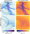 |
Fig. 1 Total gas column density (left) and line-of-sight mass-weighted CRIR (Eq. (4)) (right) for the dense (top) and diffuse (bottom) cloud models. |
3 Results and discussion
3.1 Gas and CR ionization rate distributions
Figure 1 shows the gas column densities and the line-of-sight mass-weighted CRIR,
 (4)
(4)
for both dense and diffuse clouds. We see that there is a strong correlation of the gas column density with the mass-weighted CRIR along the line-of-sight. There is an order of magnitude variation of the CRIR throughout the cloud due to the attenuation. Figure 2 shows the column density integrated along the Z axis4 for the carbon cyclespecies we consider for the two different clouds. Figure 3 summarizes the velocity-integrated line emission of [CII] 158μm, [CI] 609μm, and CO (J = 1−0) for both clouds. We discuss the aforementioned results in more detail below.
Figure 4 shows the 2D-PDF distribution, hereafter referred to as a “phase space”, of CRIR and density for the dense and diffuse clouds. The distribution shows that low-density regions encounter a CRIR an order of magnitude greater than at the highest densities. The overall trends can be explained by a self-gravitating cloud with turbulence-induced porosity, such that lower density gas is more likely to be closer to the edge of the domain and dense gas is typically found in more embedded regions in the cloud. The two clouds show remarkable similarities in the distribution functions for the same density range.
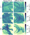 |
Fig. 2 Summary of the carbon-cycle column densities for the dense (left) and diffuse (right) cloud using the ζ(N) model. |
3.2 The average ζ – nH relation
Here, we discuss the average ζ – nH relation in both clouds and the implications for a more general relation. Numerous previous theoretical investigations have found an average trend between the effective (local) AV,eff and the total H-nucleus number density, nH, (see e.g., Glover et al. 2010; Van Loo et al. 2013; Safranek-Shrader et al. 2017; Seifried et al. 2017; Bisbas et al. 2019; Hu et al. 2021). Figure 5 shows the AV,eff − nH distribution for the two simulations along with a best fit function from Bisbas et al. (2019, and in prep):
![Mathematical equation: \begin{equation*}A_{\textrm{V, eff}}(n_{\textrm{H}}) = A_{\textrm{V,0}} \exp \left [a \left (\frac{n_{\textrm{H}}}{\textrm{cm}^{-3}} \right)^{\gamma} \right],\end{equation*}](/articles/aa/full_html/2022/02/aa42411-21/aa42411-21-eq9.png) (5)
(5)
where AV,0 = 0.05, a = 1.6, and γ = 0.12, and where for typical dust properties AV,eff and NH are related through N∕AV = 1.6 × 1021 cm−2 ≡ f (Bohlin et al. 1978; Weingartner & Draine 2001; Röllig et al. 2007; Rachford et al. 2009). We find that the best fit function reasonably reproduces the average trends in our distribution functions. A further discussion of the AV,eff – nH relation is deferred to Bisbas et al. (2019) (in particular their Appendix B and Fig. B.1) and Bisbas et al. (in prep).
Combining Eqs. (1) and (5), we get an analytic equation for the mean relationship of the attenuated CRIR and the density in the gas. We get:
![Mathematical equation: \begin{equation*}\log_{\textrm{10}} \left(\frac{\zeta}{\textrm{s}^{-1}} \right) = \sum_{k =0}^9 c_k \left[A+B \left(\frac{n_{\textrm{H}}}{\textrm{cm}^{-3}} \right)^{\gamma} \right]^k,\end{equation*}](/articles/aa/full_html/2022/02/aa42411-21/aa42411-21-eq10.png) (6)
(6)
where A = log10(fAV,0) = 19.90, B = alog10e = 0.69, γ = 0.12 (Eq. (5)), and the ck coefficients are the same as in Eq. (1) and they are given in Table 1. This ζ − nH relation is shown in Fig. 4 (red-dashed curve). This simple prescription is able to reproduce the average behavior of the two-dimensional distribution for both clouds. The universality of the ζ − nH relation is rooted at the universality of the AV,eff − nH relation, which is found to be remarkably robust across seven orders of magnitude in density, and it is seen in various simulation codes (the AV,eff − nH relation does, however, depend on metallicity; see Hu et al. 2021). We note that this trend is likely to hold only in the limit that the CR flux is relatively isotropic, that the transport is dominated by energy losses and not turbulent diffusion (and thus only dependent on the column density), and that there are no embedded sources of CRs.
Due to the similarity of the ζ – nH phase space between the two clouds and of their AV,eff – nH phase spaces, we expect the qualitative impact of CR attenuation to be similar. Therefore, in the rest of this paper, we focus only on the dense cloud simulation.
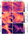 |
Fig. 3 Summary of the carbon-cycle line-of-sight integrated fluxes for the dense (left) and diffuse (right) cloud using the ζ(N) model. |
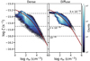 |
Fig. 4 Local CR ionization rate – density 2D-PDF for the dense and diffuse clouds. The red line is a parameterization utilizing an AV,eff–nH relation (seeEq. (5)) and the black dashed line is the analytic equation by Eq. (6). |
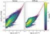 |
Fig. 5 AV,eff – nH 2D-PDF for the dense and diffuse clouds. The red-line is the AV,eff–nH relation (seeEq. (5)). |
3.3 Impact on the distribution of carbon cycle species
We first discuss the impact of CR attenuation on the distribution of C+, C, and CO. Figure 6 shows the column densities of C+, C, and CO for the ζ(N) model and the relative differences in the column densities, defined by
 (7)
(7)
for a given species, i, with a constant CRIR, ζc, relative to the ζ(N) model. We find that the ζc = 5 × 10⁻¹⁶ s−1 model significantly overproduces C+ and C and underproduces CO, while the ζc = 10−16 s−1 model underproduces C+ and C but overproduces CO. The model with ζc = 2 × 10⁻¹⁶ s−1 has the minimal error. The behavior of CO is interesting; the ζc = 5 × 10⁻¹⁶ s−1 model overproduces CO in diffuse regions while underproducing CO in a thin zone surrounding the dense gas structures. This trend is flipped for the ζc = 2 × 10⁻¹⁶ and 5 × 10⁻¹⁶ s−1 models. At high densities, the CO distributions are effectively identical.
Figures 7–9 show the x(C+) − n, x(C) − n, and x(CO) − n phase spaces, for our various simulations with the bin averages as red lines. The last panel on the bottom right of each figure shows the linear-relative error in the average abundance profiles for a specific constant CRIR model compared to the ζ(N) model.
Looking at Figs. 7–9, we can identify several general trends. First, for densities nH ≲ 100 cm−3, the abundance of C+ is insensitive to the ζ. This is because gas at these densities is preferentially located near the cloud boundary (following Eq. (5), this gas has AV eff ≤ 0.8, on average) where carbon photoionization is efficient and dominates the production of C+ 5. In this regime, photoionization keeps the carbon predominantly in ionized form, with x(C+) ≃ AC ≈ 10−4, where AC is the elemental carbon abundance.
Then, as we move to higher densities, we sampled regions at higher AV, at which point dust absorption becomes important, significantly reducing the efficiency of carbon photoionization. At nH ≫ 100 cm−3, CR-driven reactions dominate over photoionization and the C+ abundance then depends on ζ. In this regime, as the CRIR increases, the abundances of both C and C+ increase, at the expense of CO. This is because CRs (1) ionize He resulting in the formation of He+, and (2) excite H2 molecules generating FUV radiation inside the cloud interior (Sternberg et al. 1987; Gredel et al. 1989; Heays et al. 2014; Bialy 2020). Both the He+ ions and the FUV CR produced an FUV radiation result in the destruction of CO molecules and the formation of C and C+. Similarly, for very high CRIRs, the induced FUV radiation can become an important source of C+ through the photoionization of C. Thus, the abundances of C and C+ generally increase with ζ. For a thorough discussion of these chemical reactions, readers can refer to Sect. 2.3 in Bialy & Sternberg (2015), and also their Sect. 5 for analytic scaling relations (in particular, their Eq. (45)).
Indeed, looking at Figs. 7–8, we see that within this high-density regime, the C and C+ abundances are always higher for the two models with high CRIRs (ζc = (5, 10) × 10−16 s−1), compared to the ζ(N) model (at these densities, the ζ(N) model gives a CRIR that is typically below 5 × 10⁻¹⁶ s−1; see Fig. 4).
Looking at the bottom-right panels of Figs. 7–8, we see that as the density increases, the relative abundances of C and C+ (in each of the ζc models, relative to the ζ(N) model) increase with increasing ζc. At sufficiently high densities, even the models with ζc = 2 × 10⁻¹⁶ s−1 and ζc = 10−16 s−1 exhibit higher C and C+ abundances, compared to the ζ(N) model. This is because while the CRIR remains constant in the ζc models, it decreases with nH in the ζ(N) model, as seen in Fig. 4 (see also Eq. (6)). Specifically, at the points nH ≈ 5 × 10³ and 105 cm−3, the CRIR in the ζ(N) model falls below the values of the two constant CRIR models, ζc = 2 × 10⁻¹⁶ s−1 and ζc = 10−16 s−1, respectively. These are the points where there is a transition from underproduction to overproduction of C and C+ in the ζc = (1, 2) × 10−16 s−1 models (compared to the ζ(N) model), that is, the curves in the bottom-right panels cross zero.
Looking at Fig. 9, we see that while the region where the CO abundance is sensitive to ζ is limited to low and intermediatedensities, that is nH ≲ 104 cm−3, nH ≈ 104 cm−3 CO becomes essentially independent of ζ. This is because even though CRs drive the destruction processes of CO, at these high densities, the CO formation rate strongly exceeds the destruction rate (the CO formation-to-destruction rate ratio increases with nH ∕ζ). Thus, the carbon becomes predominantly in the form of CO, and the CO abundance saturates at the elemental carbon abundance, xCO ≈ AC.
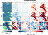 |
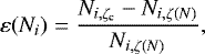
Fig. 6 Carbon cycle column density for the ζ(N) model and deviations in the calculated column densities for different ζc. First column: column densities of ionized carbon (top), neutral carbon (middle), and carbon monoxide (bottom) for our nonconstant ζ(N) model. Second to fourth columns: relative difference (see Eq. (7)) in column density for a constant CRIR with respect to the ζ(N) model for each of the aforementioned species. |
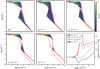 |
Fig. 7 C+ abundance, x(C+) versus hydrogen nuclei density, nH. The CR model is annotated in each panel. The red lines denote the binned averaged abundance profiles in log–log space. The dashed-dotted lines shows the ζ(N) abundance profile for comparison. Bottom right panel: relative error of the average abundance profiles. |
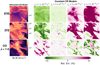 |
Fig. 10 Line-of-sight integrated flux for each carbon cycle species for the ζ(N) model and deviations in the integrated flux from models using different ζc. First column: velocity-integrated emission of the [CII] 158 μm (top), [CI] 609 μm (middle), and CO (1–0) (bottom) emission in units of (K km s−1). Second to fourth columns: relative emission for the different constant CR ionization rate models with respect to the ζ(N) model. |
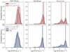 |
Fig. 11 PDFs of the velocity-integrated emission of [CII] 158 μm (left), [CI] 609μm (center), and CO (1–0) (right) for the different ionization rate models. The vertical lines highlight the peak emission. |
3.4 Variations in the observed emission
We now investigate the impact of CR attenuation on the velocity-integrated line emissions of [CII] 158μm, [CI] 3P1 → 3P0 at 609 μm, and the 12CO J =1−0 (hereafter ‘CO (1–0)’) rotational transition at 115.27 GHz. Figure 10 shows the [CI] 609 μm and CO (1–0) integrated emission and the relative errors of these with different constant CRIRs compared to the ζ(N) model.
We find that the 5 × 10⁻¹⁶ s−1 model is overly bright in [CII] 158 μm and [CI] 609 μm, while 10−16 s−1 is too dim. For [CI] 609 μm, there is a low-density pocket in which these trends are flipped. For CO (1–0), the ζc = 5 × 10⁻¹⁶ s−1 model is too dim in diffuse gas regions, while being over-bright in dense gas (compared to the ζ(N) model). This trend is flipped in the ζc = 10−16 s−1 model.
Figure 11 shows probability density functions (PDFs) of the distribution of the emission of [CII] 158 μm, [CI] 609 μm, and CO (1–0). For [CI] 609 μm, the distribution at the low end is nearly identical, while there are significant deviations for bright regions. The peak brightness changes drastically with different constant ionization rates, highlighting the issues with modeling C chemistry and emission with a constant ionization rate. However, the distributions of the [CI] 609 μm emission for the ζ(N) and ζc = 2 × 10⁻¹⁶ models are nearly identical. This trend is matched by the CO emission, where there is a broad distribution of high emission which is very sensitive to the constant CRIR chosen. For the [CII] 158μm emission, none of the constant CRIR models represent the distribution in the ζ(N) model well, although the mass-weighted ζc = 2 × 10⁻¹⁶ s−1 matches both the peak and the distribution best.
The physical reason behind the changing [CI] 609 μm emission peaks lies in the contrast between the gas temperature and the excitation temperature. The decrease in the emission peak is due to the dense-gas (nH > 103 cm−3) temperature dropping below hν∕kB ≃ 23.1 K, which is the temperature associated with the energy of the [CI] forbidden-line emission at 609 μm (see Appendix A). Thus, choosing a CRIR to match the diffuse gas produces higher temperatures in the dense gas. It is worth reminding that the temperatures calculated here are not self-consistent with the Hu et al. (2021) results. Their CRIR was scaled linearly with the local star-formation rate, without attenuation being included.
Our current analysis has focused on a single projection, along the Z axis, of the cloud. Here, we evaluate the impact of different lines of sight. In Fig. 12, we show the [CI] 609 μm integrated flux distribution for different projections Fig. 12 shows that the distributions are relatively similar, although there is more dim emission in the other projections. The X- and Y-projections are nearly identical. Figure 13 shows the ratio of the total integrated flux for each ζc model with respect to the ζ(N) model for the three emission lines considered here. The blue line shows the Z-projection emission, while the red-shaded regions show the overall spread with the line of sight. For the optically thin emission, the trend of the total flux ratio for different ζc values is the same. For CO, there is greater spread, although the qualitative trends are the same with different lines of sight. The higher spread is expected due to the optical thickness of the line.
Finally, we show in Fig. 14 the CO SLED for the different CRIR models. We find that for low-J transitions, all the ζc models reproduce the line ratios well. However, toward higher-J transitions, the differences become more discrepant, due to the attenuation of the CRs resulting in different temperature distributions in dense gas. The ζc = 10−16 and 2 × 10⁻¹⁶ s−1 models give the best agreement with the ζ(N) model, whilethe higher ζc models produce too much high J-CO excitation. This is because these lower CRIR models have a mass-weighted mean temperature that is quite similar to the one seen in the ζ(N) model (see Appendix A).
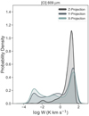 |
Fig. 12 PDFs of the velocity-integrated emission of [CI] 609 μm for three different lines of sight for the ζ(N) model. |
 |
Fig. 13 Ratios of the total integrated flux from different lines of sight for each of the CRIR models with respect to the ζ(N) model for [CII] (left), [CI] (middle), and CO (J = 1−0) (right). Theblue line denotes the ratio for the Z projection and the red band denotes the overall spread over the three lines of sight. |
 |
Fig. 14 CO SLEDS for each of the CRIR models. Left: CO line ratios between higher excitation transitions and the ground transition for the different cosmic-ray ionization rate models.Right: relative error in the CO line ratios for each ζc with respect to the ζ(N) model. |
4 Conclusions
We have presented an analysis of a post-processed photo-dissociation region model of a dense molecular cloud in which wehave included a prescription of the CRIR as a function of the local hydrogen column density, ζ(N). We find the following:
The column density projection maps of the carbon cycle species, C+, C, and CO, are significantly influenced by the inclusion of CR attenuation versus utilizing a constant ionization rate. The relative error in the column densities computed using a constant ionization rate versus an attenuated model can be greater than unity (Fig. 6). However, for deeply embedded regions, the impact on the CO column density is marginal.
The choice of a CR model has a profound impact on the resulting volumetric abundances of the carbon cycle species, ni (Figs. 7–9). This effect is particularly strong for C+ and C, with variations greater than an order of magnitude for number densities, nH > 103 cm−3.
We demonstrate that the overall velocity-integrated emission of many species is changed by imposing a column density dependent CRIR model, not only due to changes in the abundances, but also in the temperatures of the dense gas (nH > 103 cm−3) because of the volumetric nature of CR heating. In particular, we find that, irrespective of the chosen line of sight, high constant ionization rates overproduce [CII] and [CI] emission and underproduce CO (J = 1–0) emission, while the inverse is true for low constant ionization rate models. No constant ionization rate model is able to reproduce all lines simultaneously, although the rate ζc = 2 × 10⁻¹⁶ s−1 has the smallest relative errors for all projections.
For CO, the spectral line energy distribution is also impacted by the chosen CRIR model (see Fig. 14). For low-J transitions, Jup < 3, the total integrated fluxes are similar. However, for high-J transitions, there is a significant variation. Therefore, a CRIR chosen to model diffuse gas may misrepresent the emission in the dense gas.
We showed that the dense and diffuse clouds have similar distributions of the ζ − nH phase space. Under the assumption of a general AV,eff − nH relationship, the resulting ζ(nH) function reproduces the average trends shown in the ζ − nH distribution well (see Eq. (6) and Fig. 4).
In summary, we have investigated the effects of CR attenuation on the carbon-cycle chemistry, and compared them to constant CRIR models. The constant CRIR models cannot fully reproduce the behavior of the attenuated model over all regimes of densities, temperatures, and species. For the ck coefficients of Table 1 used (Padovani et al. 2018), the best match is found for ζc = 2 × 10⁻¹⁶ s−1, which reproduces the projected emission maps and columns reasonably well. However, even this model does not reproduce the local volume densities well in the simulation at high densities. Therefore, we recommend the following CRIR prescriptions, in descending order of emphasis:
If local (effective) column densities are available, a column-dependent prescription for the CRIR should be utilized (e.g., Eq. (1)); or,
if local column densities are not available, the analytic prescription in Eq. (6) for the necessary hydrogen-nuclei density for Milky Way-like environments should be utilized; or,
if neither of the above are possible, the constant CRIR, ζc = 2 × 10⁻¹⁶ s−1, should be utilized since it resulted in the smallest relative errors in the integrated line emission.
Our results represent a novel look at the impact of CR attenuation on the carbon-cycle chemistry of three-dimensional molecular clouds and the observed emission from these species. However, our treatment of CR transport is only approximate. Future studies will utilize more sophisticated CR physics to better untangle the fingerprints CR transport physics leaves of the molecular interstellar medium.
Acknowledgements
The authors thank the anonymous referee for their comments which improved the clarity of this work. The following PYTHON packages were utilized: NUMPY (Harris et al. 2020), SCIPY (Virtanen et al. 2020), MATPLOTLIB (Hunter 2007), DATASHADER, CMOCEAN. B.A.L.G. acknowledges support by the ERC starting grant No. 679852 ‘RADFEEDBACK’ and the Deutsche Forschungsgemeinschaft (DFG) via the Collaborative Research Center SFB 956 “Conditions and Impact of Star Formation”. T.G.B. acknowledges support from Deutsche Forschungsgemeinschaft (DFG) grant No. 424563772. S.B. acknowledges support from the Center for Theory and Computations (CTC) at the University of Maryland.
Appendix A Dense-gas temperature distributions
We investigate the response of the gas temperature in the nH ≥103 cm−3 regime with increasing ζ. Figure A.1 shows temperature PDFs for the various simulations including all cells with densities nH ≥103 cm−3. As expected, the distributions follow the trend that higher constant ionization rates produce warmer gas. However, only the ζc = 2 × 10⁻¹⁶ s−1 model reproduces the dense gas temperature distribution of the ζ(N) model. For observational tracers of the dense gas, the chosen ionization rate may have a significant impact on the model emission. Table A.1 shows the mass-weighted gas temperature,  (again, only including cells with nH≥103 cm−3). We find that the ζc = 10−16 s−1 and the 2 × 10⁻¹⁶ s−1 models have
  closer to the ζ(N) model. Indeed, the CO SLED for these two models best matches that of the SLED of ζ(N) (see Section 3.2).
Mass-weighted gas temperatures for different CR ionization rate models
We highlight the impact of these small changes within the 20-30 K temperature regime that have on higher-J CO transitions for nH>103 cm−3. Table A.2 shows radiation temperature (the equivalent blackbody temperature of the emission in the Rayleigh-Jeans limit6) calculations using RADEX (van der Tak et al. 2007) of the CO ladder (up to J = 10 −9) for a gas density of nH = 104 cm−3 with different gas temperatures, T = 20 and 26 K, and with N(CO) = 1018 cm−3. The aforementioned values were chosen to match with the conditions in the high-density regime as can be seen in Figs.1 and 6. Despite the relatively small difference in the average gas temperature, it has a profound impact on the predictions for the high-J transitions, with deviations up to ~40 times for the J = 10 − 9 transition. Thus, accurately modeling the temperature of the dense gas is of paramount importance in constraining the physical ISM environment from high-J CO transitions.
 |
Fig. A.1 Temperature PDFs in the dense gas (all cells with nH ≥ 103 cm−3) for the different CRIR models. |
RADEX model results for the radiation temperature, TR (K), of the CO J-ladder for nH = 104 cm−3.
References
- Accurso, G., Saintonge, A., Bisbas, T. G., & Viti, S. 2017, MNRAS, 464, 3315 [NASA ADS] [CrossRef] [Google Scholar]
- Aguilar, M., Aisa, D., Alvino, A., et al. 2014, Phys. Rev. Lett., 113, 121102 [Google Scholar]
- Aguilar, M., Aisa, D., Alpat, B., et al. 2015, Phys. Rev. Lett., 114, 171103 [CrossRef] [PubMed] [Google Scholar]
- Bayet, E., Williams, D. A., Hartquist, T. W., & Viti, S. 2011, MNRAS, 414, 1583 [NASA ADS] [CrossRef] [Google Scholar]
- Bialy, S. 2020, Commun. Phys., 3, 32 [NASA ADS] [CrossRef] [Google Scholar]
- Bialy, S., & Sternberg, A. 2015, MNRAS, 450, 4424 [NASA ADS] [CrossRef] [Google Scholar]
- Bisbas, T. G., Bell, T. A., Viti, S., Yates, J., & Barlow, M. J. 2012, MNRAS, 427, 2100 [NASA ADS] [CrossRef] [Google Scholar]
- Bisbas, T. G., Papadopoulos, P. P., & Viti, S. 2015, ApJ, 803, 37 [NASA ADS] [CrossRef] [Google Scholar]
- Bisbas, T. G., Tanaka, K. E. I., Tan, J. C., Wu, B., & Nakamura, F. 2017a, ApJ, 850, 23 [NASA ADS] [CrossRef] [Google Scholar]
- Bisbas, T. G., van Dishoeck, E. F., Papadopoulos, P. P., et al. 2017b, ApJ, 839, 90 [Google Scholar]
- Bisbas, T. G., Schruba, A., & van Dishoeck, E. F. 2019, MNRAS, 485, 3097 [NASA ADS] [Google Scholar]
- Bisbas, T. G., Tan, J. C., & Tanaka, K. E. I. 2021, MNRAS, 502, 2701 [CrossRef] [Google Scholar]
- Bohlin, R. C., Savage, B. D., & Drake, J. F. 1978, ApJ, 224, 132 [Google Scholar]
- Bolatto, A. D., Wolfire, M., & Leroy, A. K. 2013, ARA&A, 51, 207 [CrossRef] [Google Scholar]
- Bothwell, M. S., Aguirre, J. E., Aravena, M., et al. 2017, MNRAS, 466, 2825 [Google Scholar]
- Cardelli, J. A., Meyer, D. M., Jura, M., & Savage, B. D. 1996, ApJ, 467, 334 [Google Scholar]
- Cartledge, S. I. B., Lauroesch, J. T., Meyer, D. M., & Sofia, U. J. 2004, ApJ, 613, 1037 [NASA ADS] [CrossRef] [Google Scholar]
- Caselli, P., & Ceccarelli, C. 2012, A&ARv, 20, 56 [Google Scholar]
- Dalgarno, A. 2006, Proc. Natl. Acad. Sci., 103, 12269 [NASA ADS] [CrossRef] [Google Scholar]
- Fitz Axen, M., Offner, S. S. S., Gaches, B. A. L., et al. 2021, ApJ, 915, 43 [NASA ADS] [CrossRef] [Google Scholar]
- Franeck, A., Walch, S., Seifried, D., et al. 2018, MNRAS, 481, 4277 [NASA ADS] [CrossRef] [Google Scholar]
- Gaches, B. A. L., Offner, S. S. R., & Bisbas, T. G. 2019a, ApJ, 878, 105 [NASA ADS] [CrossRef] [Google Scholar]
- Gaches, B. A. L., Offner, S. S. R., & Bisbas, T. G. 2019b, ApJ, 883, 190 [NASA ADS] [CrossRef] [Google Scholar]
- Glover, S. C. O., Federrath, C., Mac Low, M. M., & Klessen, R. S. 2010, MNRAS, 404, 2 [Google Scholar]
- Grassi, T., Padovani, M., Ramsey, J. P., et al. 2019, MNRAS, 484, 161 [NASA ADS] [CrossRef] [Google Scholar]
- Gredel, R., Lepp, S., Dalgarno, A., & Herbst, E. 1989, ApJ, 347, 289 [Google Scholar]
- Grenier, I. A., Black, J. H., & Strong, A. W. 2015, ARA&A, 53, 199 [Google Scholar]
- Habing, H. J. 1968, Bull. Astron. Inst. Netherlands, 19, 421 [Google Scholar]
- Harris, C. R., Millman, K. J., van der Walt, S. J., et al. 2020, Nature, 585, 357 [NASA ADS] [CrossRef] [Google Scholar]
- Heays, A. N., Visser, R., Gredel, R., et al. 2014, A&A, 562, A61 [NASA ADS] [CrossRef] [EDP Sciences] [Google Scholar]
- Hollenbach, D. J., & Tielens, A. G. G. M. 1999, Rev. Mod. Phys., 71, 173 [Google Scholar]
- Hu, C.-Y., Sternberg, A., & van Dishoeck, E. F. 2021, ApJ, 920, 44 [NASA ADS] [CrossRef] [Google Scholar]
- Hunter, J. D. 2007, Comput. Sci. Eng., 9, 90 [NASA ADS] [CrossRef] [Google Scholar]
- Indriolo, N., & McCall, B. J. 2012, ApJ, 745, 91 [NASA ADS] [CrossRef] [Google Scholar]
- Indriolo, N., & McCall, B. J. 2013, Chem. Soc. Rev., 42, 7763 [NASA ADS] [CrossRef] [Google Scholar]
- Indriolo, N., Neufeld, D. A., Gerin, M., et al. 2015, ApJ, 800, 40 [NASA ADS] [CrossRef] [Google Scholar]
- Ivlev, A. V., Dogiel, V. A., Chernyshov, D. O., et al. 2018, ApJ, 855, 23 [NASA ADS] [CrossRef] [Google Scholar]
- Lo, N., Cunningham, M. R., Jones, P. A., et al. 2014, ApJ, 797, L17 [NASA ADS] [CrossRef] [Google Scholar]
- McElroy, D., Walsh, C., Markwick, A. J., et al. 2013, A&A, 550, A36 [NASA ADS] [CrossRef] [EDP Sciences] [Google Scholar]
- Meijerink, R., Spaans, M., Loenen, A. F., & van der Werf, P. P. 2011, A&A, 525, A119 [NASA ADS] [CrossRef] [EDP Sciences] [Google Scholar]
- Morlino, G., & Gabici, S. 2015, MNRAS, 451, L100 [NASA ADS] [CrossRef] [Google Scholar]
- Neufeld, D. A., & Wolfire, M. G. 2017, ApJ, 845, 163 [Google Scholar]
- Offner, S. S. R., Bisbas, T. G., Bell, T. A., & Viti, S. 2014, MNRAS, 440, L81 [NASA ADS] [CrossRef] [Google Scholar]
- Owen, E. R., On, A. Y. L., Lai, S.-P., & Wu, K. 2021, ApJ, 913, 52 [NASA ADS] [CrossRef] [Google Scholar]
- Padovani, M., Galli, D., & Glassgold, A. E. 2009, A&A, 501, 619 [NASA ADS] [CrossRef] [EDP Sciences] [Google Scholar]
- Padovani, M., Hennebelle, P., & Galli, D. 2013, A&A, 560, A114 [NASA ADS] [CrossRef] [EDP Sciences] [Google Scholar]
- Padovani, M., Ivlev, A. V., Galli, D., & Caselli, P. 2018, A&A, 614, A111 [NASA ADS] [CrossRef] [EDP Sciences] [Google Scholar]
- Padovani, M., Ivlev, A. V., Galli, D., et al. 2020, Space Sci. Rev., 216, 29 [CrossRef] [Google Scholar]
- Papadopoulos,P. P., Thi, W. F., & Viti, S. 2004, MNRAS, 351, 147 [NASA ADS] [CrossRef] [Google Scholar]
- Phan, V. H. M., Morlino, G., & Gabici, S. 2018, MNRAS, 480, 5167 [NASA ADS] [Google Scholar]
- Rachford, B. L., Snow, T. P., Destree, J. D., et al. 2009, ApJS, 180, 125 [NASA ADS] [CrossRef] [Google Scholar]
- Redaelli, E., Sipilä, O., Padovani, M., et al. 2021, A&A 656, A109 [NASA ADS] [CrossRef] [EDP Sciences] [Google Scholar]
- Rimmer, P. B., Herbst, E., Morata, O., & Roueff, E. 2012, A&A, 537, A7 [NASA ADS] [CrossRef] [EDP Sciences] [Google Scholar]
- Röllig, M., Abel, N. P., Bell, T., et al. 2007, A&A, 467, 187 [Google Scholar]
- Safranek-Shrader, C., Krumholz, M. R., Kim, C.-G., et al. 2017, MNRAS, 465, 885 [NASA ADS] [CrossRef] [Google Scholar]
- Schlickeiser, R. 2002, Cosmic Ray Astrophysics (Berlin: Springer) [CrossRef] [Google Scholar]
- Schlickeiser, R., Caglar, M., & Lazarian, A. 2016, ApJ, 824, 89 [NASA ADS] [CrossRef] [Google Scholar]
- Seifried, D., Walch, S., Girichidis, P., et al. 2017, MNRAS, 472, 4797 [NASA ADS] [CrossRef] [Google Scholar]
- Silsbee, K., & Ivlev, A. V. 2019, ApJ, 879, 14 [NASA ADS] [CrossRef] [Google Scholar]
- Sternberg, A., Dalgarno, A., & Lepp, S. 1987, ApJ, 320, 676 [NASA ADS] [CrossRef] [Google Scholar]
- Tielens, A. G. G. M. 2005, The Physics and Chemistry of the Interstellar Medium (Cambridge: Cambridge University Press) [Google Scholar]
- van der Tak, F. F. S., Black, J. H., Schöier, F. L., Jansen, D. J., & van Dishoeck, E. F. 2007, A&A, 468, 627 [NASA ADS] [CrossRef] [EDP Sciences] [Google Scholar]
- Van Loo, S., Butler, M. J., & Tan, J. C. 2013, ApJ, 764, 36 [NASA ADS] [CrossRef] [Google Scholar]
- Virtanen, P., Gommers, R., Oliphant, T. E., et al. 2020, Nat. Methods, 17, 261 [Google Scholar]
- Weingartner, J. C., & Draine, B. T. 2001, ApJ, 548, 296 [Google Scholar]
- Wu, B., Tan, J. C., Nakamura, F., et al. 2017, ApJ, 835, 137 [NASA ADS] [CrossRef] [Google Scholar]
- Zhang, Z.-Y., Henkel, C., Gao, Y., et al. 2014, A&A, 568, A122 [NASA ADS] [CrossRef] [EDP Sciences] [Google Scholar]
Hereafter, we refer to species abundances and densities through parentheses, and to elemental abundances through subscripts.
For implementation into FORTRAN codes, it is heavily advised to use 16 digit precision reals to avoid numerical inaccuracy after the logarithm is exponentiated.
Throughout this paper, projection plots integrate along the Z axis unless otherwise stated.
The ionization potential of C is hν = 11.3 eV. Thus, even in regions where the hydrogen is predominantly neutral (i.e., in the bulk of the ISM), carbon may be readily photoionized by photons with energies in the range hν = (11.3−13.6) eV.
RADEX defines this as the main beam antennae temperature with a beam filling factor of unity.
All Tables
Polynomial coefficients, ck for Eqs. (1) and (6), from Table F.1 from Padovani et al. (2018).
RADEX model results for the radiation temperature, TR (K), of the CO J-ladder for nH = 104 cm−3.
All Figures
|
Fig. 1 Total gas column density (left) and line-of-sight mass-weighted CRIR (Eq. (4)) (right) for the dense (top) and diffuse (bottom) cloud models. |
| In the text | |
|
Fig. 2 Summary of the carbon-cycle column densities for the dense (left) and diffuse (right) cloud using the ζ(N) model. |
| In the text | |
|
Fig. 3 Summary of the carbon-cycle line-of-sight integrated fluxes for the dense (left) and diffuse (right) cloud using the ζ(N) model. |
| In the text | |
|
Fig. 4 Local CR ionization rate – density 2D-PDF for the dense and diffuse clouds. The red line is a parameterization utilizing an AV,eff–nH relation (seeEq. (5)) and the black dashed line is the analytic equation by Eq. (6). |
| In the text | |
|
Fig. 5 AV,eff – nH 2D-PDF for the dense and diffuse clouds. The red-line is the AV,eff–nH relation (seeEq. (5)). |
| In the text | |
|
Fig. 6 Carbon cycle column density for the ζ(N) model and deviations in the calculated column densities for different ζc. First column: column densities of ionized carbon (top), neutral carbon (middle), and carbon monoxide (bottom) for our nonconstant ζ(N) model. Second to fourth columns: relative difference (see Eq. (7)) in column density for a constant CRIR with respect to the ζ(N) model for each of the aforementioned species. |
| In the text | |
|
Fig. 7 C+ abundance, x(C+) versus hydrogen nuclei density, nH. The CR model is annotated in each panel. The red lines denote the binned averaged abundance profiles in log–log space. The dashed-dotted lines shows the ζ(N) abundance profile for comparison. Bottom right panel: relative error of the average abundance profiles. |
| In the text | |
 |
Fig. 8 As in Fig. 7, but for C. |
| In the text | |
 |
Fig. 9 As in Fig. 7, but for CO. |
| In the text | |
|
Fig. 10 Line-of-sight integrated flux for each carbon cycle species for the ζ(N) model and deviations in the integrated flux from models using different ζc. First column: velocity-integrated emission of the [CII] 158 μm (top), [CI] 609 μm (middle), and CO (1–0) (bottom) emission in units of (K km s−1). Second to fourth columns: relative emission for the different constant CR ionization rate models with respect to the ζ(N) model. |
| In the text | |
|
Fig. 11 PDFs of the velocity-integrated emission of [CII] 158 μm (left), [CI] 609μm (center), and CO (1–0) (right) for the different ionization rate models. The vertical lines highlight the peak emission. |
| In the text | |
|
Fig. 12 PDFs of the velocity-integrated emission of [CI] 609 μm for three different lines of sight for the ζ(N) model. |
| In the text | |
|
Fig. 13 Ratios of the total integrated flux from different lines of sight for each of the CRIR models with respect to the ζ(N) model for [CII] (left), [CI] (middle), and CO (J = 1−0) (right). Theblue line denotes the ratio for the Z projection and the red band denotes the overall spread over the three lines of sight. |
| In the text | |
|
Fig. 14 CO SLEDS for each of the CRIR models. Left: CO line ratios between higher excitation transitions and the ground transition for the different cosmic-ray ionization rate models.Right: relative error in the CO line ratios for each ζc with respect to the ζ(N) model. |
| In the text | |
|
Fig. A.1 Temperature PDFs in the dense gas (all cells with nH ≥ 103 cm−3) for the different CRIR models. |
| In the text | |
Current usage metrics show cumulative count of Article Views (full-text article views including HTML views, PDF and ePub downloads, according to the available data) and Abstracts Views on Vision4Press platform.
Data correspond to usage on the plateform after 2015. The current usage metrics is available 48-96 hours after online publication and is updated daily on week days.
Initial download of the metrics may take a while.