| Issue |
A&A
Volume 658, February 2022
|
|
|---|---|---|
| Article Number | A62 | |
| Number of page(s) | 8 | |
| Section | Planets and planetary systems | |
| DOI | https://doi.org/10.1051/0004-6361/202142077 | |
| Published online | 01 February 2022 | |
KMT-2018-BLG-1988Lb: Microlensing super-Earth orbiting a low-mass disk dwarf
1
Department of Physics, Chungbuk National University,
Cheongju
28644,
Republic of Korea
e-mail: This email address is being protected from spambots. You need JavaScript enabled to view it.
2
Department of Astronomy, Tsinghua University,
Beijing
100084,
PR China
3
Max Planck Institute for Astronomy,
Königstuhl 17,
69117
Heidelberg,
Germany
4
Department of Astronomy, The Ohio State University,
140 W. 18th Ave.,
Columbus,
OH
43210,
USA
5
University of Canterbury, Department of Physics and Astronomy,
Private Bag 4800,
Christchurch
8020,
New Zealand
6
Korea Astronomy and Space Science Institute,
Daejon
34055,
Republic of Korea
7
Department of Particle Physics and Astrophysics, WeizmannInstitute of Science,
Rehovot
76100,
Israel
8
Center for Astrophysics,
Harvard & Smithsonian 60 Garden St.,
Cambridge,
MA
02138,
USA
9
School of Space Research, Kyung Hee University,
Yongin,
Kyeonggi
17104,
Republic of Korea
10
Department of Astronomy & Space Science, Chungbuk National University,
Cheongju
28644,
Republic of Korea
Received:
24
August
2021
Accepted:
15
November
2021
Abstract
Aims. We reexamine high-magnification microlensing events in the previous data collected by the KMTNet survey with the aim of finding planetary signals that were not noticed before. In this work, we report the planetary system KMT-2018-BLG-1988L, which was found from this investigation.
Methods. The planetary signal appears as a deviation with ≲0.2 mag from a single-lens light curve and lasted for about 6 h. The deviation exhibits a pattern of a dip surrounded by weak bumps on both sides of the dip. The analysis of the lensing light curve indicates that the signal is produced by a low-mass-ratio (q ~ 4 × 10⁻⁵) planetary companion located near the Einstein ring of the host star.
Results. The mass of the planet, Mplanet = 6.8−3.5+4.7 M⊕ and 5.6−2.8+3.8 M⊕ for the two possible solutions, estimated from the Bayesian analysis indicates that the planet is in the regime of a super-Earth. The host of the planet is a disk star with a mass of Mhost = 0.47−0.25+0.33 M⊙ and a distance of DL = 4.2−.14+1.8 kpc. KMT-2018-BLG-1988Lb is the 18th known microlensing planet with a mass below the upper limit of a super-Earth. The fact that 15 out of the 18 known microlensing planets with masses ≲10 M⊕ were detected in the 5 yr following the full operation of the KMTNet survey indicates that the KMTNet database is an important reservoir of very low-mass planets.
Key words: gravitational lensing: micro / planets and satellites: detection
© ESO 2022
1 Introduction
Microlensing searches for planets are being conducted by inspecting light curves of the more than 3000 lensing events that are detected annually by massive lensing surveys monitoring stars lying in the Galactic bulge field. Planetary signals in lensing light curves appear as short-lasting perturbations to the lensing light curves produced by the planet hosts. Some planetary signals may escape detection for two major reasons. The first is the short duration of a signal relative to the cadence of observations. The duration of a planetary signal becomes shorter as the mass ratio q between the planet and host decreases, and thus signals of lower-mass planets are more likely to be missed. The second cause arises due to the weakness of planetary signals. A majority of published planetary signals are produced by the crossings of source stars over planet-induced caustics, and the signals produced via this caustic-crossing channel tend to be strong. However, planetary signals produced via a non-caustic-crossing channel tend to be weak and may escape detection (Zhu et al. 2014). Planetary signals can also be weak if lensing events are affected by severe finite-source effects or involve faint source stars.
Complete detections of planets that include short and weak signals are important for the accurate estimation of the planet frequency and a solid demographic census of microlensing planetary systems. The basis for the statistical assessment of these planet properties is the detection efficiency, which is assessed as the ratio of the number of events with detected planets to the total number of lensing events, as done, for example, in Gould et al. (2010). If a planetary signal is missed despite its strength being above the detection threshold, the efficiency would be underestimated, and this would subsequently lead to the erroneous estimation of planet properties.
From a series of projects conducted during the COVID-19 period, microlensing data collected in previous years were reinvestigated for the purpose of finding missing planets. The reinvestigation was carried out via two approaches. The first approach was visually inspecting lensing light curves with weak or short anomaly features. From the visual reinvestigation of faint-source lensing events in the 2016–2017 season data, Han et al. (2020) reported four microlensing planets (KMT-2016-BLG-2364Lb, KMT-2016-BLG-2397Lb, OGLE-2017-BLG-0604Lb, and OGLE-2017-BLG-1375Lb), for which the planetary signals had not been noticed due to the weakness of the signals caused by the faintness of source stars. From the reexamination of the 2018–2019 season data, Han et al. (2021a,b) reported the detections of four planets (KMT-2018-BLG-1025Lb, KMT-2018-BLG-1976Lb, KMT-2018-BLG-1996Lb, and OGLE-2019-BLG-0954Lb), for which the planetary signals were missed due to their weakness caused by the non-caustic-crossing nature. The second approach was applying an automated algorithm to the previous data to search for buried signals of planets. Application of this algorithm to the 2018–2019 prime-field data of the Korea Microlensing Telescope Network (KMTNet; Kim et al. 2016) survey by Zang et al. (2021b) and Hwang et al. (2022) led to the discoveries of six planets (OGLE-2018-BLG-0977Lb, OGLE-2018-BLG-0506Lb, OGLE-2018-BLG-0516Lb, OGLE-2019-BLG-1492Lb, and KMT-2019-BLG-0253, OGLE-2019-BLG-1053) with weak and short signals. The automated searches for short and weak planetary signatures is planned to be extended to the data of the entire KMTNet fields.
In this work, we report the discovery of a super-Earth planet detected from the systematic reinvestigation of high-magnification lensing events conducted with the aim of finding missing planets in the 2018 season data obtained by the KMTNet survey. The planet was not noticed before because its signal was not only weak but also short due to its non-caustic-crossing origin and the very small planet/host mass ratio.
For the presentation of the planet discovery, we organize the paper according to the following structure. In Sect. 2, we describe the observation of the lensing event and the data used in the analysis. In Sect. 3, we depict the procedure of the lensing light curve analysis and present the lens system configuration found from the analysis. We also mention the degeneracy encountered in the interpretation of the lensing event. In Sect. 4, we investigate the possibility of measuring higher-order lensing observables. In Sect. 5, we define the source type by measuring the color and magnitude and estimate the angular Einstein radius. In Sect. 6, we describe the Bayesian analysis conducted to estimate the physical lens parameters. We summarize the result and conclude in Sect. 7.
2 Observations and data
The planet was detected from the analysis of the lensing event KMT-2018-BLG-1988. The source star of the event is located toward the Galactic bulge field with equatorial coordinates (RA, Dec)J2000 = (17:41:07.81, − 35:35:40.92), which corresponds to the galactic coordinates (l, b) = (−6°.168, −2°.686).
The lensing event was detected from the post-season inspection of the 2018 KMTNet data using the EventFinder algorithm (Kim et al. 2018). The source was located in the KMTNet field BLG37, which was covered with a 2.5 h cadence. This cadence was substantially lower than that of the KMTNet prime fields, for which the cadence was 15 min. The field corresponds to the BLG610 field of the Optical Gravitational Lensing Experiment (OGLE: Udalski et al. 2015), but no OGLE microlensing observation was conducted for this field in the 2018 season.
Observations of the event by the KMTNet survey were carried out using the three telescopes that are located at the Siding Spring Observatory (KMTA) in Australia, the Cerro Tololo Inter-American Observatory (KMTC) in Chile, and the South African Astronomical Observatory (KMTS) in South Africa. The telescopes are identical with a 1.6 m aperture, and each telescope is mounted with a camera yielding 2 × 2 deg2 field of view.Images were taken mainly in the I band, and a fraction of V -band images were obtained for the source color measurement.
Reduction of the images and photometry of the source were done using the KMTNet pipeline developed by Albrow et al. (2009). The pipeline is a customized version of the pySIS code established based on the difference imaging method (Tomaney & Crotts 1996; Alard & Lupton 1998). The error bars of the photometry data assessed by the automatized pipeline were readjusted using the method described in Yee et al. (2012) in order for them to be consistent with the scatter of data and to make the χ2 per degree of freedom for each data set unity. For a subset of KMTC I- and V -band data, additional photometry was done utilizing the pyDIA software (Albrow 2017) to construct the color-magnitude diagram (CMD) of stars around the source and to measure the reddening- and extinction-corrected (dereddened) source color and brightness. We describe the detailed procedure of the source color measurement in Sect. 5.
Figure 1 shows the lensing light curve of KMT-2018-BLG-1988 constructed with the combined data from the three KMTNet telescopes. At first glance, it appears to show a smooth and symmetric form of an event produced by a single-mass lens magnifying a single source (1L1S). Drawn over the data points is the 1L1S model curve with the lensing parameters (u0, tE) ~ (0.014, 50 days), where u0 denotes the lens-source separation (scaled to the angular Einstein radius θE) at the time of the closest lens-source approach t0, and tE is the event timescale. The full lensing parameters of the 1L1S model is presented in Table 1. The event was highly magnified with a peak magnification of Apeak ~ 1∕u0 ~ 70. A close lookat the region around the peak, shown in the inset of Fig. 1 and the top panel of Fig. 2, reveals that there exists a short-term anomaly. The anomaly exhibits deviations with ≲ 0.2 mag from the 1L1S model and lasted for about 6 h. The anomaly was found from the close inspection of the event conducted in the project of reexamining high-magnification events in the previous KMTNet data. In this project, high-magnification events are selected as targets for close examination due to their high sensitivities to planets (Griest & Safizadeh 1998).
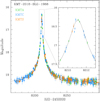 |
Fig. 1 Lensing light curve of KMT-2018-BLG-1988. The inset shows the zoom-in view of the peak region. The curve superposed on the data points is the single-lens single-source (1L1S) model. The colors of data points are set to match those of the telescopes marked in the legend. |
Lensing parameters of tested models.
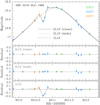 |
Fig. 2 Data around the peak region of the lensing light curve and three tested model curves: 2L1S (close), 2L1S (wide), and 1L1S. Three lower panels: residuals from the individual models. The curve drawn in the bottom panel represents the difference between the close 2L1S model and the 1L1S model. |
3 Light curve analysis
The signature of the anomaly comes mainly from the two KMTC points acquired at the epochs of HJD′≡HJD − 2 450 000 = 8210.719 and 8210.776, which exhibit deviations from the 1L1S model of ΔI = −0.182 mag (compared to the photometric uncertainty of σI = 0.026 mag) and − 0.132 mag (σI = 0.026 mag), respectively. The KMTS point at HJD′ = 8210.617 (with ΔI = +0.032 mag) and the KMTC point at HJD′ = 8210.863 (with ΔI = +0.057 mag) also show deviations, although the signals are weaker than the previous two points. We designate the four points taken at HJD′ = 8210.617, 8210.719, 8210.776, and 8210.863 as t1, t2, t3, and t4, respectively. The residuals from the 1L1S model, presented in the bottom panel of Fig. 2, show that the points at t2 and t3 manifest negative deviations, while the data points at t1 and t4 exhibit slight positive deviations, and thus the anomaly appears to be a dip surrounded by weak bumps on both sides of the dip.
We checked whether the anomaly were attributed to some kinds of correlated noise, for example, fake signals due to correlations with seeing. For this check, we examined the image quality of these data points and compared the quality with that of adjacent data points. The upper three panels of Fig. 3 show the difference images obtained by subtracting a template image taken before the lensing magnification from the object images of the three anomalous KMTC points (at t2, t2, and t3), and they are compared to the other three images taken about one day after the anomaly (at HJD′ = 8211.718, 8211.776, and 8211.863). In the panels, we insert the seeing (FWHM) values of the individual images. We find that the quality of the images taken during the anomaly is similar to that of the images obtained after the anomaly, indicating that there is no noticeable correlations with seeing. There exists a saturated bright star on the lower left side of the source, but we find that it does not affect the photometry of the source. Therefore, we conclude that the anomaly is real.
The fact that the anomaly lasted for a short period of time and it occurred near the peak of a high-magnification event suggests thepossibility that the anomaly was produced by a planetary companion. The fact that the anomaly does not exhibit a sharp spike indicates that the source did not cross a planet-induced caustic. The anomaly pattern characterized by a dip surrounded by shallow bumps suggests that the anomaly was produced by the source star’s passage through the planet-host axis on the opposite side of the planet. Example planetary lensing events with similar anomaly patterns are found in OGLE-2018-BLG-0677 (Herrera-Martín et al. 2020), KMT-2018-BLG-1976, KMT-2018-BLG-1996 (Han et al. 2021a), KMT-2019-BLG-0253, OGLE-2018-BLG-0506, OGLE-2018-BLG-0516, and OGLE-2019-BLG-0149 (Hwang et al. 2022). The possibility of a binary-source interpretation (Gaudi 1998; Gaudi & Han 2004) for the origin of the anomaly is excluded because a source companion produces only positive deviations, while the observed anomaly exhibits a negative deviation.
Considering the possible planet origin of the anomaly, we conduct a binary-lens (2L1S) modeling for the observed light curve. A 2L1S lensing light curve is described by 7 parameters: t0, u0, tE, s, q, α, and ρ. The first three (t0, u0, tE) are 1L1S parameters describing the lens-source approach, and the next three parameters (s, q, α) characterize the binary lens, denoting the projected separation (scaled to θE) and mass ratio between the lens components (M1 and M2), and the source trajectory angle defined as the angle between the direction of the source motion and M1 –M2 axis, respectively. The last parameter (normalized source radius), defined as the ratio of the angular source radius θ* to the Einstein radius, that is, ρ = θ*∕θE, is included to account for finite-source effects during caustic crossings, although the anomaly is unlikely to be produced by a caustic crossing.
In the 2L1S modeling, we divide the lensing parameters into two groups, in which (s, q) in the first group are searched for using a grid approach, while the other parameters in the second group are searched for via a downhill approach. We use the Markov chain Monte Carlo (MCMC) algorithm for the downhill approach. Because a central anomaly can be produced not only by a planetary companion lying near the Einstein ring but also by a wide or a close binary companion with a similar mass to that of the primary lens (Han & Gaudi 2008), we set the ranges of the grid parameters s and q wide enough, − 1.0 ≤ logs < 1.0 and − 5.5 ≤ logq < 1.0, to check the binary origin of the anomaly. From this first-round modeling, we identify local solutions in the Δχ2 map on the s–q plane. In the second-round modeling, we refine the identified local solutions by releasing all parameters as free parameters.
In Table 1, we list the lensing parameters of the solutions found from the 2L1S modeling conducted under the assumption of a rectilinear relative lens-source motion (standard model). We identify two local solutions with sclose ~ 0.97 (close solution) and swide ~ 1.01 (wide solution), indicating that the companion to the lens is located very close to the Einstein ring regardless of the solution. The estimated lens mass ratio is on the order of 10−5, indicating that the companion to the lens is a very low-mass planet. The model curves of the solutions are drawn over the data points and the residuals from the solutions are presented in Fig. 2. Both the close and wide 2L1S models explain all the anomalous points, improving the fit with Δχ2 ~ 80 relative to the 1L1S model.
In Fig. 4, we present the lens system configurations, which show the source trajectory (the curve with an arrow) with respect to the caustic (red concave closed figure), of the close (upper panel) and wide (lower panel) solutions. We note that the presented configurations are for the models considering higher-order effects causing non-rectilinear lens-source motion to be discussedbelow, but the configurations of the standard models are very similar to the presented ones. As predicted from the pattern and location, the anomaly was generated by the passage of the source through the negative anomaly region formed around the planet-host axis on the opposite side of the planet. We mark the positions of the source at the four epochs of the anomaly: t1, t2, t3, and t4. The two KMTC data points at t2 and t3 correspond to the epochs of the source passage through the negative perturbation region, and the other two points at t1 and t4 correspond to the epochs when the source passed the positive perturbation regions extending from the back-end cusps of the caustic.
The degeneracy between the close and wide solutions is very severe with Δχ2 = 0.1. The type of the degeneracy is similar to that identified by Yee et al. (2021), who found that there existed a continuous transition between the two well-known types of degeneracy in planetary lensing events: “close–wide” (Griest & Safizadeh 1998; Dominik 1999; An 2005) and “inner–outer” (Gaudi & Gould 1997) degeneracies. A planetary companion induces two types of caustics, in which one is located close to the planet host (central caustic) and the other lies away from the host (planetary caustic). The close-wide degeneracy arises due to the similarity between the two central caustics of the solutions with s < 1.0 and s > 1.0. The inner-outer degeneracy arises due to the similarity between the two light curves resulting from the source trajectories passing the inner (with respect to the primary) and outer region of the planetary caustic. From the geometry of the source trajectory with respect to the central caustic, on one hand, the light curve of KMT-2018-BLG1988 is subject to the close–wide degeneracy because the source approached the central caustic. From the geometry of the source trajectory relative to the planetary caustic, on the other hand, the light curve is also subject to the inner–outer degeneracy because the source passed the outer (right) and inner (left) region of the planetary caustic, as shown in the insets of the individual panels of Fig. 4. As a result, the degeneracy is caused by the combination of the two types of degeneracy.
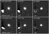 |
Fig. 3 Difference images of the data points taken during (upper three panels) and one day after the anomaly (lower panels). The labels in the upper and lower left side of each image indicate the time of the image acquisition and seeing (FWHM). |
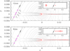 |
Fig. 4 Lens system configurations for the close (upper panel) and wide (lower panel) 2L1S models. In each panel, the curve with an arrow is the source trajectory and the cuspy close figures represent the caustics. The caustic shape varies depending on time due to the variation in the M1 –M2 separation induced by the lens orbital motion, and the presented caustic is the one corresponding to the time of the anomaly, that is, HJD′~ 8107.7. The gray curves around the caustic are the equi-magnification contours. The four empty circles on the source trajectory drawn in magenta color represent the source locations at t1 = 8210.617, t2 = 8210.719, t3 = 8210.776, and t4 = 8210.863. The size of the circle is arbitrarily set and not scaled to the source size. The inset in each panel shows a wider view including both central and planetary caustics. |
4 Higher-order effects
The physical parameters of the mass M and distance DL to the lens can be constrained by measuring the lensing observables including the event timescale tE, angular Einstein radius θE, and microlens-parallax πE. The first two observables are related to M and DL by
 (1)
(1)
where μ represents the relative lens-source proper motion, κ = 4G∕(c2AU),  is the relative lens-source parallax, and DS denotes thedistance to the source star. The additional measurement of πE would enable one to uniquely determine M and DL by
 (2)
(2)
where πS = AU∕DS represents the annual parallax of the source star (Gould 2000). The event timescale is measured from the light curve modeling and presented in Table 1. The Einstein radius is estimated by θE = θ*∕ρ, where ρ is measured from the analysis of the deviations in the lensing light curve caused by finite-source effects, and θ* is deduced from the source color and brightness. We discuss in detail the procedure of determination in the following section. The microlens parallax is measured from the deviation of the light curve caused by the non-rectilinear lens-source motion induced by the orbital motion of Earth around the Sun (Gould 1992). For the measurement πE, we conduct an additional modeling considering the microlens-parallax effect. In this modeling, we also consider the orbital motion of the lens (Dominik 1998), which is known to produce similar deviations to those induced by the parallax effect (Batista et al. 2011). The inclusion of the higher-order effects in modeling requires one to include two extra pairs of lensing parameters: (πE,E, πE,N) and (d s∕dt, dα∕dt). The first pair denote the north and east components of the microlens parallax vector πE = (πrel∕θE)(μ∕μ), respectively, and the other pair represent the annual change rates of the binary separation and source trajectory angle, respectively.
The lensing parameters obtained from the modeling considering the higher-order effects (higher-order 2L1S model) are listed in Table 1. We find that the consideration of the higher-order effects improves the fit by Δχ2 ~ 11 with respect to the standard models. It is found that finite-source effects cannot be firmly detected because the source did not cross the caustic. Nevertheless, the upper limit of ρ can be placed. The left panel of Fig. 5 shows the distribution of points in the MCMC chain (scatter plot) on the u0 –ρ parameter plane. We set a conservative upper limit as ρmax = 0.003. The right panel of Fig. 5 shows the scatter plot on the πE,E–πE,N plane. It shows that the uncertainties of the parallax parameters are big, especially the north component πE,N. Similarly, the uncertainties of the orbital parameters are considerable.
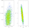 |
Fig. 5 Scatter plots on the u0–ρ (left panel) and πE,E–πE,N (right panel)planes. The color coding is set to represent points with <1σ (red), <2σ (yellow), <3σ (green), <4σ (cyan), and <5σ (blue). |
5 Source star
For the estimation of the angular Einstein radius, we specify the source type by measuring its dereddened color and brightness,  . In order to measure
  from the uncalibratedvalues, (V − I, I), in the instrumental color-magnitude diagram (CMD), we use the Yoo et al. (2004) method, in which the centroid of red giant clump (RGC) is used for calibration.
Figure 6 shows the source location (empty circle with error bars) with respect to the RGC centroid (red filled dot) in the instrumental CMD of stars around the source constructed using the pyDIA photometry of the KMTC I- and V -band data. Also marked is the location of the blend (green filled dot). The measured instrumental colors and magnitudes of the source and RGC centroid are (V − I, I) = (2.462 ± 0.063, 21.248 ± 0.002) and  , respectively.From the offsets in color and magnitude between the source and RGC centroid, Δ(V − I, I), together with the known dereddened values of theRGC centroid
  from Bensby et al. (2013) and Nataf et al. (2013), we estimate the dereddened color and magnitude of the source as
 (3)
(3)
indicating that the spectral type of the source is K2V.
The angular source radius is estimated by first converting the measured V − I color into V − K color using the color-color relation of Bessell & Brett (1988), and then deduce θ* from the (V − K)–θ* relation of Kervella et al. (2004). From this procedure, it is estimated that the source has an angular radius of
 (4)
(4)
Combined with the measured event timescale and the upper limit of the normalized source radius, the lower limits of the Einstein radius and the relative lens-source proper motion are set as
 (5)
(5)
and
 (6)
(6)
respectively.
We checked whether a significant fraction of the blended light comes from the lens. The flux from a lens contributes to the blended flux, and thus if the lens is bright enough, the lens can be additionally constrained by analyzing the blended flux, for example, the planetary events OGLE-2018-BLG-1269 (Jung et al. 2020a) and OGLE-2018-BLG-0740 (Han et al. 2019). For this check, we measured the astrometric offset between the baseline object and the source. The position of the source was measured from the difference images obtained during lensing magnifications. The measured offsets in the east and north directions are Δθ(E, N) = (37.2 ± 5.6, 370.0 ± 4.8) mas. The offset is well beyond the measurement error, indicating that the blended flux is likely to come from an adjacent star unrelated to lensing. Considering that the blend lies on the main-sequence branch of disk stars, it is unlikely that the blend is a binary companion to the source that lies in the bulge. This is also supported by the fact that the lens brightness expected from the mass and distance, to be estimated in the next section, is much fainter than the brightness of the blend.
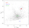 |
Fig. 6 Source location (blue empty dot) with respect to the centroid of red giant clump (RGC, filled red dot) in the color-magnitude diagram constructed using the pyDIA photometry of the KMTC data. Also marked is the location of the blend (green filled dot). |
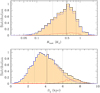 |
Fig. 7 Bayesian posterior distributions of the planet host mass and distance to the lens. In each panel, the blue and red curves indicate the contributions by the disk and bulge lens populations. The solid vertical line represents the median of the distribution and the two dotted lines denote 1σ range of the distribution. |
Physical lens parameters.
6 Physical parameters of planetary system
We estimate the physical parameters of the planetary system based on the measured lensing observables. Among the lensing observables of (tE, θE, πE), the event timescale is relatively well constrained, but the uncertainty of the microlens parallax is substantial, and only the upper limit of the Einstein radius is constrained, making it difficult to uniquely determine M and DL using the relation in Eq. (2). We, therefore, estimate the physical lens parameters by conducting a Bayesian analysis using the constraints from the observables together with a prior Galactic model.
In the Bayesian analysis, we first conduct a Monte Carlo simulation to produce a large number (2 × 10⁶) of artificial lensing events, for which the locations of the lens and source, lens-source transverse speeds, v⊥, and lens masses are derived from the Galactic model. The Galactic model is constructed by adopting the Han & Gould (2003) physical distribution,Han & Gould (1995) dynamical distribution, and Zhang et al. (2020) mass function of Galactic objects. The further description about the Galactic model is found in Jung et al. (2021). For the individual simulated events, we compute lensing observables by tE = DLθE∕v⊥,  , and πE = πrel∕θE, and then construct the posterior distributions of the lens mass and distance for the events with observables lying within the ranges of the observed values.
Figure 7 shows the posterior distributions of the planet host mass and distance to the planetary system. In Table 2, we summarize the masses of the host, Mhost, and planet, Mplanet, distance, and projected host-planet separation, a⊥, estimated based on the lensing parameters of the close and wide solutions. For each parameter, the median of the Bayesian distribution is taken as a represent value, and the lower and upper limits are set as the 16 and 84% of the distribution, respectively. The estimated mass,  for the close solution and
  for the wide solution, indicates that the planet is in the regime of a super-Earth, which is defined as a planet with a mass higher than the mass of Earth, but substantially lower than those of the Solar System’s ice giants, that is, Uranus and Neptune (Valencia et al. 2007). The mass of the planet host,
  , indicates that the host is a late K or an early M dwarf. The estimated distance to the lens,
  kpc, suggests that the lens is likely to lie in the disk. According to the Bayesian estimation of the disk (blue curve in Fig. 7) and bulge (red curve) contributions, the probability of a disk lens is ~ 82%. We note that the uncertainties of the estimated physical lens parameters are considerable due to the combination of the statistical nature of the Bayesian analysis and the weak constraints of lensing observables. Furthermore, the estimated parameters can vary depending on adopted models (Yang et al. 2021).
The planetary system KMT-2018-BLG-1988L demonstrates the importance of high-cadence microlensing surveys in finding low-mass planets. By setting the upper mass limit of a super-Earth as ~ 10 M⊕, there exist 18 microlensing planetary systems with planet masses lower than this upper limit, including the system reported in this work. In Table 3, we list these planets discovered so far from the lensing surveys that have been conducted for almost three decades. In the table, we list the masses of planets and hosts together with the references and brief comments for notable systems. We note that the list is arranged according to the chronological order of the lensing event discovery not by the times of the planet discovery. Among these discovered planets, 15 planets have been found since 2016, when the KMTNet survey conducted its full operation, indicating that the KMTNet database is an important reservoir of low-mass microlensing planets.
Microlensing planets with masses of less than 10 M⊕.
7 Conclusion
We reported the super-Earth planet KMT-2018-BLG-1988L detected from the reinvestigation of high-magnification events in the previous microlensing data collected by the KMTNet survey. The planetary signal appeared as a deviation with ≲ 0.2 mag from a 1L1Scurve and lasted for about 6 h. The analysis of the lensing light curve indicated that the signal was produced by a low-mass-ratio planetary companion located at around the Einstein ring of the host star. The mass of the planet,  and
and  for the two possible solutions, estimated from the Bayesian analysis indicated that the planet was in the regime of a super-Earth. The planet belonged to a disk star with a mass of
  located at a distance of
 kpc. KMT-2018-BLG-1988L is the 18th microlensing planet discovered with a mass below the upper limit of a super-Earth. The fact that 15 out of the 18 known planets with masses ≲ 10 M⊕ were detected in the 5 yr following the full operation of the KMTNet survey indicates that the KMTNet database is an important reservoir of very low-mass planets.
Acknowledgements
Work by C.H. was supported by the grants of National Research Foundation of Korea (2020R1A4A2002885 and 2019R1A2C2085965). This research has made use of the KMTNet system operated by the Korea Astronomy and Space Science Institute (KASI) and the data were obtained at three host sites of CTIO in Chile, SAAO in South Africa, and SSO in Australia.
References
- Alard, C., & Lupton, R. H. 1998, ApJ, 503, 325 [Google Scholar]
- Albrow, M. 2017, https://doi.org/10.5281/zenodo.268049 [Google Scholar]
- Albrow, M., Horne, K., Bramich, D. M., et al. 2009, MNRAS, 397, 2099 [Google Scholar]
- An, J. H. 2005, MNRAS, 356, 1409 [Google Scholar]
- Batista, V., Gould, A., Dieters, S., et al. 2011, A&A, 529, A102 [NASA ADS] [CrossRef] [EDP Sciences] [Google Scholar]
- Beaulieu, J.-P., Bennett, D. P., Fouqué, P., et al. 2006, Nature, 439, 437 [Google Scholar]
- Bennett, D. P., Bond, I. A., Udalski, A., et al. 2008, ApJ, 684, 663 [Google Scholar]
- Bensby, T., Yee, J. C., Feltzing, S., et al. 2013, A&A, 549, A147 [NASA ADS] [CrossRef] [EDP Sciences] [Google Scholar]
- Bessell, M. S.,& Brett, J. M. 1988, PASP, 100, 1134 [Google Scholar]
- Blackman, J. W., Beaulieu, J.-P., Cole, A. A., et al. 2021, AJ, 161, 279 [NASA ADS] [CrossRef] [Google Scholar]
- Bond, I. A., Bennett, D. P., Sumi, T., et al. 2017, MNRAS, 469, 2434 [Google Scholar]
- Dominik, M. 1998, A&A, 329, 361 [NASA ADS] [Google Scholar]
- Dominik, M. 1999, A&A, 349, 108 [NASA ADS] [Google Scholar]
- Gaudi, B. S. 1998, ApJ, 506, 533 [Google Scholar]
- Gaudi, B. S., & Gould, A. 1997, ApJ, 486, 85 [Google Scholar]
- Gaudi, B. S., & Han, C. 2004, ApJ, 611, 528 [NASA ADS] [CrossRef] [Google Scholar]
- Gould, A. 1992, ApJ, 392, 442 [Google Scholar]
- Gould, A. 2000, ApJ, 542, 785 [NASA ADS] [CrossRef] [Google Scholar]
- Gould, A., Dong, S., Gaudi, B. S., et al. 2010, ApJ, 720, 1073 [NASA ADS] [CrossRef] [Google Scholar]
- Gould, A., Udalski, A., Shin, I.-G., et al. 2014, Science, 345, 46 [Google Scholar]
- Gould, A., Ryu, Y.-H., Calchi Novati, S., et al. 2020, J. Kor. Astron. Soc., 53, 9 [NASA ADS] [Google Scholar]
- Griest, K., & Safizadeh, N. 1998, ApJ, 500, 37 [Google Scholar]
- Han, C., & Gould, A. 1995, ApJ, 447, 53 [Google Scholar]
- Han, C., & Gould, A. 2003, ApJ, 592, 172 [Google Scholar]
- Han, C., & Gaudi, B. S. 2008, ApJ, 689, 53 [CrossRef] [Google Scholar]
- Han, C., Yee, J. C., Udalski, A., et al. 2019, AJ, 158, 102 [NASA ADS] [CrossRef] [Google Scholar]
- Han, C., Udalski, A., Kim, D., et al. 2020, A&A, 642, A110 [EDP Sciences] [Google Scholar]
- Han, C., Udalski, A., Kim, D., et al. 2021a, A&A, 650, A89 [NASA ADS] [CrossRef] [EDP Sciences] [Google Scholar]
- Han, C., Udalski, A., Lee, C.-U., et al. 2021b, A&A, 649, A90 [EDP Sciences] [Google Scholar]
- Herrera-Martín, A., Albrow, M. D., Udalski, A., et al. 2020, AJ, 159, 256 [Google Scholar]
- Hwang, K.-H., Zang, W., Gould, et al. 2022, AJ, 163, 43 [NASA ADS] [CrossRef] [Google Scholar]
- Jung, Y. K., Gould, A., Udalski, A., et al. 2020a, AJ, 160, 148 [NASA ADS] [CrossRef] [Google Scholar]
- Jung, Y. K., Udalski, A., Zang, W., et al. 2020b, AJ, 160, 255 [Google Scholar]
- Jung, Y. K., Han, C., Udalski, A., et al. 2021, AJ, 161, 293 [NASA ADS] [CrossRef] [Google Scholar]
- Kervella, P., Thévenin, F., Di Folco, E., & Ségransan, D. 2004, A&A, 426, 29 [Google Scholar]
- Kim, S.-L., Lee, C.-U., Park, B.-G., et al. 2016, J. Kor. Astron. Soc., 49, 37 [NASA ADS] [CrossRef] [Google Scholar]
- Kim, D.-J., Kim, H.-W., Hwang, K.-H., et al. 2018, AJ, 155, 76 [Google Scholar]
- Kondo, I., Yee, J. C., Bennett, D. P., et al. 2021, AJ, 162, 77 [NASA ADS] [CrossRef] [Google Scholar]
- Mróz, P., Poleski, R., Gould, A., et al. 2020, ApJ, 903, L11 [Google Scholar]
- Nataf, D. M., Gould, A., Fouqué, P., et al. 2013, ApJ, 769, 88 [Google Scholar]
- Ryu, Y.-H., Udalski, A., Yee, J. C., et al. 2020, AJ, 160, 183 [Google Scholar]
- Shvartzvald, Y., Yee, J. C., Calchi Novati, S., et al. 2017, ApJ, 840, L3 [Google Scholar]
- Tomaney, A. B., & Crotts, A. P. S. 1996, AJ, 112, 2872 [Google Scholar]
- Udalski, A., Szymański, M. K., & Szymański, G. 2015, Acta Astron., 65, 1 [NASA ADS] [Google Scholar]
- Udalski, A., Ryu, Y.-H., Sajadian, S., et al. 2018, Acta Astron., 68, 1 [Google Scholar]
- Valencia, D., Sasselov, D. D., & O’Connell, R. J. 2007, ApJ, 656, 545 [Google Scholar]
- Yang, H., Mao, S., Zang, W., & Zhang, X. 2021, MNRAS, 502, 5631 [NASA ADS] [CrossRef] [Google Scholar]
- Yee, J. C., Shvartzvald, Y., Gal-Yam, A., et al. 2012, ApJ, 755, 102 [Google Scholar]
- Yee, J. C., Zang, W, Udalski, A., et al. 2021, AJ, 162, 180 [NASA ADS] [CrossRef] [Google Scholar]
- Yoo, J., DePoy, D. L., Gal-Yam, A., et al. 2004, ApJ, 603, 139 [Google Scholar]
- Zang, W., Han, C., Kondo, I., et al. 2021a, Res. Astron. Astrophys., 9, 239 [CrossRef] [Google Scholar]
- Zang, W., Hwang, K.-H., Udalski, A., et al. 2021b, AJ, 162, 163 [NASA ADS] [CrossRef] [Google Scholar]
- Zhang, X., Zang, W., Udalski, A., et al. 2020, AJ, 159, 116 [Google Scholar]
- Zhu, W., Penny, M., Mao, S., Gould, A., & Gendron, R. 2014, ApJ, 788, 73 [Google Scholar]
All Tables
All Figures
|
Fig. 1 Lensing light curve of KMT-2018-BLG-1988. The inset shows the zoom-in view of the peak region. The curve superposed on the data points is the single-lens single-source (1L1S) model. The colors of data points are set to match those of the telescopes marked in the legend. |
| In the text | |
|
Fig. 2 Data around the peak region of the lensing light curve and three tested model curves: 2L1S (close), 2L1S (wide), and 1L1S. Three lower panels: residuals from the individual models. The curve drawn in the bottom panel represents the difference between the close 2L1S model and the 1L1S model. |
| In the text | |
|
Fig. 3 Difference images of the data points taken during (upper three panels) and one day after the anomaly (lower panels). The labels in the upper and lower left side of each image indicate the time of the image acquisition and seeing (FWHM). |
| In the text | |
|
Fig. 4 Lens system configurations for the close (upper panel) and wide (lower panel) 2L1S models. In each panel, the curve with an arrow is the source trajectory and the cuspy close figures represent the caustics. The caustic shape varies depending on time due to the variation in the M1 –M2 separation induced by the lens orbital motion, and the presented caustic is the one corresponding to the time of the anomaly, that is, HJD′~ 8107.7. The gray curves around the caustic are the equi-magnification contours. The four empty circles on the source trajectory drawn in magenta color represent the source locations at t1 = 8210.617, t2 = 8210.719, t3 = 8210.776, and t4 = 8210.863. The size of the circle is arbitrarily set and not scaled to the source size. The inset in each panel shows a wider view including both central and planetary caustics. |
| In the text | |
|
Fig. 5 Scatter plots on the u0–ρ (left panel) and πE,E–πE,N (right panel)planes. The color coding is set to represent points with <1σ (red), <2σ (yellow), <3σ (green), <4σ (cyan), and <5σ (blue). |
| In the text | |
|
Fig. 6 Source location (blue empty dot) with respect to the centroid of red giant clump (RGC, filled red dot) in the color-magnitude diagram constructed using the pyDIA photometry of the KMTC data. Also marked is the location of the blend (green filled dot). |
| In the text | |
|
Fig. 7 Bayesian posterior distributions of the planet host mass and distance to the lens. In each panel, the blue and red curves indicate the contributions by the disk and bulge lens populations. The solid vertical line represents the median of the distribution and the two dotted lines denote 1σ range of the distribution. |
| In the text | |
Current usage metrics show cumulative count of Article Views (full-text article views including HTML views, PDF and ePub downloads, according to the available data) and Abstracts Views on Vision4Press platform.
Data correspond to usage on the plateform after 2015. The current usage metrics is available 48-96 hours after online publication and is updated daily on week days.
Initial download of the metrics may take a while.