| Issue |
A&A
Volume 658, February 2022
|
|
|---|---|---|
| Article Number | A77 | |
| Number of page(s) | 10 | |
| Section | Extragalactic astronomy | |
| DOI | https://doi.org/10.1051/0004-6361/202040133 | |
| Published online | 03 February 2022 | |
A MUltiwavelength Study of ELAN Environments (AMUSE2)
Ubiquitous dusty star-forming galaxies associated with enormous Lyα nebulae on megaparsec scales
1
Department of Physics, Colorado College, 14 E. Cache La Poudre Street, Colorado Springs, CO 80903, USA
2
Academia Sinica Institute of Astronomy and Astrophysics (ASIAA), No. 1, Sec. 4, Roosevelt Rd., Taipei 10617, Taiwan
e-mail: This email address is being protected from spambots. You need JavaScript enabled to view it.
3
Max-Planck-Institut fur Astrophysik, Karl-Schwarzschild-Str 1, 85748 Garching bei München, Germany
4
Dipartimento di Fisica G. Occhialini, Università degli Studi di Milano Bicocca, Piazza della Scienza 3, 20126 Milano, Italy
5
Centre for Extragalactic Astronomy, Durham University, South Road, Durham DH1 3LE, UK
6
Institute for Computational Cosmology, Durham University, South Road, Durham DH1 3LE, UK
7
Department of Astronomy, Tsinghua University, Beijing 100084, PR China
8
Dipartimento di Fisica e Astronomia, Università di Firenze, Via G. Sansone 1, 50019 Sesto Fiorentino, Firenze, Italy
9
INAF – Osservatorio Astrofisico di Arcetri, 50125 Florence, Italy
10
UCO/Lick Observatory, University of California, 2013 Santa Cruz, Santa Cruz, CA 95064, USA
11
Kavli Institute for the Physics and Mathematics of the Universe (Kavli IPMU), 5-1-5 Kashiwanoha, Kashiwa 277-8583, Japan
12
Korea Astronomy and Space Science Institute, 776 Daedeokdae-ro, Yuseong-gu, Daejeon 34055, Republic of Korea
Received:
15
December
2020
Accepted:
25
October
2021
Abstract
We have been undertaking a systematic survey at 850 μm based on a sample of four prototypical z ∼ 2 − 3 enormous Lyα nebulae (ELANe) as well as their megaparsec-scale (Mpc-scale) environments to study the physical connections between ELANe and their coeval dusty submillimeter galaxies (SMGs). By analysing the SCUBA-2 data with self-consistent Monte Carlo simulations to construct the number counts, here, we report on the overabundance of 850 μm-selected submillimeter sources around all the four ELANe, by a factor of 3.6 ± 0.6 (weighted average) compared to the blank fields. This suggests that the excessive number of submillimeter sources are likely to be part of the Mpc-scale environment around the ELANe, corroborating the co-evolution scenario for SMGs and quasars; this is a process which may be more commonly observed in the ELAN fields. If the current form of the underlying count models continues toward the fainter end, our results would suggest an excess of the 850 μm extragalactic background light by a factor of between 2–10, an indication of significant background light fluctuations on the survey scales. Finally, by assuming that all the excessive submillimeter sources are associated with their corresponding ELAN environments, we estimate the SFR densities of each ELAN field, as well as a weighted average of ΣSFR = 1200 ± 300 M⊙ yr−1 Mpc−3, consistent with that found in the vicinity of other quasar systems or proto-clusters at similar redshifts; in addition, it is a factor of about 300 greater than the cosmic mean.
Key words: galaxies: clusters: general / galaxies: halos / galaxies: high-redshift / cosmic background radiation / submillimeter: galaxies
© ESO 2022
1. Introduction
Galaxies that are selected at submillimeter wavelengths, in particular at 850 micron, contain sites that exhibit some of the most intensive star formation across the Universe, with estimated star-formation rates up to thousands of solar masses per year (e.g., Barger et al. 2012; Swinbank et al. 2014; Cowie et al. 2017; Dudzevičiūtė et al. 2020). They are predominantly located at z = 1 − 3, with a long tail toward z > 4 (Barger et al. 2000; Chapman et al. 2005; Wardlow et al. 2011; Simpson et al. 2014; Chen et al. 2016a; Stach et al. 2018; Dudzevičiūtė et al. 2020; Smail et al. 2021), matching the trend of cosmic star formation rate (SFR) densities (Madau & Dickinson 2014). Evidence that has been collected since the discovery of the first submillimeter galaxies (SMGs; Smail et al. 1997; Barger et al. 1998; Hughes et al. 1998) points to an evolutionary scenario whereby these massive (1010–1011 M⊙ in stellar masses; da Cunha et al. 2015; Michałowski et al. 2017) dusty star-forming galaxies would evolve into the likes of local massive elliptical galaxies, undergoing subsequent multiple phase transitions that include optically bright quasars, compact quiescent galaxies, and dry mergers (e.g., Toft et al. 2014).
The latest evidence supporting this hypothetical evolution comes from galaxy clustering analyses, which have been enabled thanks to the sufficiently large-scale submillimeter surveys that have only recently become available (e.g., Geach et al. 2017). These studies have found, via the measurements of both auto-correlation functions and cross-correlation functions, that SMGs are predominantly located in dark-matter halos with masses of around 1012–1013 M⊙ at z ∼ 1 − 3 (Hickox et al. 2011; Chen et al. 2016a,b; Wilkinson et al. 2017; An et al. 2019; García-Vergara et al. 2020; Lim et al. 2020). This is consistent with their being the predicted progenitors of local massive elliptical galaxies, as is the case for the bright quasars at similar redshifts (White et al. 2012; Timlin et al. 2018, and references therein).
In general, subsequent active black hole accretion that coincides with or follows intensive star-forming events has long been proposed, even in the local Universe (e.g., Hopkins et al. 2006), to partly explain the rapid quenching of star formation through feedback. This hypothesis, together with the clustering analyses, would suggest an intimate co-evolution between black hole growth and star formation, such that detecting star formation in and around quasar host galaxies is expected. Indeed, the correlated signals found via cross-correlation analyses between infrared background measurements and quasar samples have further supported, on average, the co-existing nature of the two populations on halo scales (Wang et al. 2015). In addition, targeted submillimeter observations on well-defined AGN samples have revealed overdensities of submillimeter sources, as indicated by excessive submillimeter source counts, around some high-redshift radio galaxies (e.g., Stevens et al. 2003; Dannerbauer et al. 2014), as well as IR luminous AGN selected by the WISE satellite (e.g., Jones et al. 2017), again suggesting the possible co-evolution and co-existence of both active black hole accretion and dusty star formation on Mpc scales around massive halos. However, these studies have often reported overdensity only in a few fields over a larger parent sample, casting the question that the co-evolution may not be universal and can only occur under certain conditions or preferentially around a certain type of quasar (Rigby et al. 2014; Zeballos et al. 2018).
To improve our understanding of this co-evolution and to expand the quasar types studied, as part of the A MUltiwavelngth Study of ELAN Environment (AMUSE2; Arrigoni Battaia et al. 2021; Chen et al. 2021), we have been conducting submillimeter observations around Enormous Lyman Alpha nebulae (ELANe). ELANe represent the extreme of known Lyα nebulae with exceptionally bright (SBLyα ∼ 10−17 erg s−1 cm−2 arcsec−2) Lyα emission over > 100 kpc in physical scales, normally embodying multiple powering sources such as AGN, quasars, and other galaxy populations. Current statistics show that only ∼4% of bright quasars are associated with ELANe, translating into a number density of few times 10−6 Mpc−3 (Arrigoni Battaia et al. 2019, 2021; Cai et al. 2019). Spectral analyses focusing on the powering of ELANe have suggested a large amount of cool and dense gas (≳1010 M⊙ and ≳1 cm−3; Arrigoni Battaia et al. 2015; Hennawi et al. 2015), a finding that is further strengthened by the detection of molecular gas via CO in the circumgalactic medium (CGM) around a central group of galaxies in the MAMMOTH-I ELAN (Emonts et al. 2019). ELANe therefore represent one of the ideal quasar samples for a comprehensive study of the co-evolution between SMGs and quasars and extending the studies to one of the rarest and likely densest regimes.
Our first results intriguingly show a factor of four in overdensities for submillimeter sources around one ELAN, MAMMOTH-1 (z = 2.32; Cai et al. 2017; Arrigoni Battaia et al. 2018a). In this paper, we report our results on three more ELANe, the Jackpot nebula (z = 2.04; Hennawi et al. 2015), the Slug nebula (z = 2.28; Cantalupo et al. 2014), and the Fabulous nebula (z = 3.17; Arrigoni Battaia et al. 2018b), the first discovered ELANe that marked the start of studies regarding this new class of Lyman alpha nebulae. We present our data and analyses in Sects. 2 and 3, along with a summary and discussion of the impact of our results in Sect. 4. We assume the cosmological parameters H0 = 70 km s−1 Mpc−1, ΩM = 0.3, and ΩΛ = 0.7. In this cosmology, 1″ corresponds to about 7.6–8.4 physical kpc at the redshift range of our sample (Table 1). All distances reported in this work are proper. Finally, in this paper we define overdensity as nsrc/nfield, in which nsrc is the number density of the submillimeter sources in the ELAN fields and nfield is that for the blank fields.
Information of the four ELANe in our sample, along with their best-fit parameters for the underlying counts models formulated as Schecter functions.
2. Observations and data reduction
The dataset for the four ELAN fields studied in this work were acquired with the Submillimetre Common-User Bolometer Array 2 (SCUBA-2; Holland et al. 2013) on the James Clerk Maxwell Telescope (JCMT) during flexible observing in 2017 September 02,16,17,23,24, 2018 January 16-18, February 12 and March 29 (programs ID: M17BP024, M18AP054) under good weather conditions (τ225 GHz ≤ 0.06). For each target, the observations covered a field-of-view of ≃13.7′ in diameter using a DAISY scanning pattern centered on each ELAN position. Each field was scheduled with cycles (scans) of about 30 minutes, resulting in 3 hours (6 scans) for the MAMMOTH-1, the Slug and the Jackpot ELANe, while in 2.7 hours (5 scans) for the Fabulous ELAN. Even though SCUBA-2 acquires simultaneously data at 850 and 450 μm, here we focus only on the dataset at longer wavelengths as the 450 μm dataset is not deep enough to obtain proper number counts.
The data reduction follows the method outlined in Chen et al. (2013a) and Arrigoni Battaia et al. (2018a), which rely on the Dynamic Iterative Map Maker (DIMM) included in the SMURF package from the STARLINK software (Jenness et al. 2010; Chapin et al. 2013). Each scan has been reduced adopting the standard configuration file, dimmconfig_blank_field.lis, which is best for our science purposes. The coaddition of the reduced scans into final maps was then performed with the MOSAIC_JCMT_IMAGES recipe in PICARD, the Pipeline for Combining and Analyzing Reduced Data (Jenness et al. 2008).
Point source detectability is increased by applying a standard matched filter to these final maps. For this purpose, we used the PICARD recipe SCUBA2_MATCHED_FILTER. As a last step, we adopted the standard conversion factor for 850 μm (537 Jy pW−1), with upwards of 10% correction for flux calibration. The uncertainty of the flux conversion factor at 850 μm is typically 5% (Dempsey et al. 2013).
The final noise level at the centers of our maps (ELAN positions) is 0.88, 0.97, 1.02, 1.01 mJy beam−1, respectively, for the MAMMOTH-1, the Jackpot, the Slug, and the Fabulous ELANe. In this work, we focus on effective areas characterized by noise levels smaller than 2.5 times this central noise (Table 1 and white curves in Fig. 1).
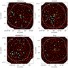 |
Fig. 1. SCUBA-2 signal-to-noise maps at 850 μm for the Fabulous, Jackpot, MAMMOTH-1, and Slug ELANe (yellow star). Sources detected at over 4σ are marked by cyan circles, and the size of the circles represents 2× the FWHM of the beam. The white curve bounds the effective area of every map, which is about 10′ (∼5 Mpc) in diameter. The quasars that contribute significantly to the powering of the corresponding ELAN are marked as yellow stars (coordinates in Table 1). |
Furthermore, we produced a true noise map (jackknife map) for each field by subtracting two maps, each representing the sum of approximately half of that source’s dataset. Therefore, the residual map should represent source-free noise data because all real sources should be subtracted irrespective of their significance. Importantly, we multiply these true noise maps by the scaling factor  with t1 and t2 being the exposure time of each pixel from the two maps, to correct for the difference in exposure time. The central noise in these jackknife maps is consistent with the noise in the science data (0.88, 0.95, 1.03, 1.01 mJy beam−1, respectively, for MAMMOTH-1, the Jackpot, the Slug, and the Fabulous ELANe).
3. Differential number counts
We extracted point sources from the SCUBA-2 maps by following the procedure from Chen et al. (2013a). The source extraction algorithm identifies the pixel with the highest signal-to-noise ratio (S/N) and subtracts a scaled point spread function (PSF) centered at the location of that pixel. The process continues until the highest S/N in the map falls below the detection threshold. In all four ELAN fields, we detect 73 sources with > 4σ located within effective areas of the maps. The locations of the detected sources, plotted over (S/N) maps, are shown in Fig. 1, and their relevant information is listed in Tables A.1–A.4.
To obtain the raw number counts, we first sum the number of sources in every flux bin and divide the sum by the width and detectable area of the bin. The detectable area is defined as the region of the map within which the sources with a given flux density can be detected above the S/N threshold. The flux bins are roughly in equal partition in logarithmic scale between the minimum and maximum flux densities of the detected sources. To correct for the detection of spurious sources, counts obtained from the jackknife maps using the same procedure are subtracted off, and the results are the raw number counts. The number of sources detected in the jackknife maps can be used to determine the fraction of spurious detections, which is 40% at the simulation threshold of 2.5σ, and 7% at the catalog threshold of 4σ.
The raw number counts are affected by observational biases, including flux boosting, source blending, and incompleteness. Instead of making corrections for these biases separately, we chose to account for these effects altogether through Monte Carlo simulations. Our goal in the simulations is to determine underlying count models that correctly reproduce the raw number counts in every field. We chose to model the differential number counts using a Schechter function of the form
 (1)
(1)
where N0 is the normalization and S0 is the characteristic flux.
The Schechter function or a double power-law function have been typically adopted for analyzing submillimeter number counts (e.g., Chen et al. 2013a; Geach et al. 2017). Here, the Schechter function is preferred over a double power-law because of a smaller number of free parameters involved. It is also the model adopted by the fiducial blank-field counts and, thus, more straightforward comparisons can be made. Experimentally, we find that the Schechter function reproduces the distribution of faint fluxes in our sample more accurately. We note, however, that the choice of the function does not significantly affect our results.
Accurate positional information and low contamination rates are not critical for statistical analyses of number counts (Chen et al. 2013a). To probe the faintest sources in our data set, we looked for the lowest detection threshold corresponding to statistically significant excess counts. The adopted detection threshold of 2.5σ is consistent with the excess in the positive signal, which is evident in Fig. 2.
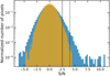 |
Fig. 2. Histogram of signal-to-noise ratio for pixels located within the effective area of the Jackpot map (blue) and the corresponding jackknife map (yellow). The solid vertical line represents the 2.5σ cut used in our simulations. The dashed line represents the threshold of 4σ above which we catalog sources. We note that the excessive negative signals compared to the jackknife map are a result of matched filtering, which can be properly accounted for during source extraction processes using a correct PSF. |
The simulation proceeds as follows. First, we fit the Schechter function to raw number counts using the least-squares method. The obtained initial parameters are used to populate the jackknife map with mock sources. The positions of mock sources are selected randomly. The lowest fluxes we inject are 1 mJy, the same as that adopted by the fiducial blank-field model (Geach et al. 2017) that we later use to compare our results. At this value, the integrated flux density of our models is statistically consistent with the extragalactic background light (EBL; e.g., Puget et al. 1996). Our results are not, in fact, sensitive to the adopted flux levels of the faintest injected sources. For a given set of model parameters, we create 100 simulated maps and calculate the mean recovered counts. The ratios of the raw counts to mean recovered counts, which are typically different in different flux bins, are used to create a new set of counts by multiplying the raw counts by these ratios. This new set of adjusted counts are then used for the next round of Schechter function fitting, for which the best fit is adopted as the new input model for the next iteration of the simulations. For each field, the process is repeated until the convergence, which is when the recovered counts fall within 1σ error of the raw counts.
The parameters of the underlying models obtained through this procedure are listed in Table 1. Given the limited dynamical range of the measured counts, N0 and S0 tend to be degenerate. We therefore keep the value of S0 fixed to 2.5, same as the fiducial blank-field model (Geach et al. 2017), but the other two parameters free. By doing so, we confirm that the simulations can converge and the results from each run are consistent with each other. We also confirm that changing S0 to other values does not significantly alter the results. To verify our methods, we run the same analyses on the SCUBA-2 images of one known blank field, CDF-N, and we confirm that CDF-N shows no evidence of overdensity, which is consistent with the published results (Chen et al. 2013a).
We tested whether the models determined through Monte Carlo simulations reproduce the raw number counts. We created 500 simulated maps for each ELAN field by injecting sources into the respective jackknife map according to the derived counts model. The mean recovered counts along with 90% confidence intervals are shown in Fig. 3. We find good agreements between the simulated counts and the raw counts in all four ELAN fields, confirming that our Monte Carlo simulations have properly accounted for observational biases. We note that the brightest bin in MAMMOTH-1 ELAN contains only two sources and its counts do not, in fact, differ substantially from the model; however, given the low probability of chance detection, they are often suspected to be associated with the ELAN system (Arrigoni Battaia et al. 2018a).
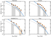 |
Fig. 3. Differential number counts recovered from 500 realizations of the number counts models determined through Monte Carlo simulations (orange) and the fiducial model (gray). The shaded regions represent the 90% confidence intervals of the counts recovered from the simulated maps. The black points are raw differential number counts, as defined in Sect. 3. The underlying counts models and the fiducial model (Geach et al. 2017) are plotted in blue and gray, respectively. The effect of flux boosting can be observed as the shaded regions are lying above their input model. We note that the lower zero limits of the fiducial model realizations at faint fluxes reflect the non-uniform noise structure of our maps, where incompleteness increases with the distance, from the center of the map. |
To further verify that our procedure is able to constrain the overdensity, we constructed another set of 500 simulated maps using a blank field model. By injecting sources into the jackknife maps following a blank-field model, we simulated the number counts that would have been observed in each of the four fields if an overdensity were not present. As a blank field model, we selected the Schechter function from Geach et al. (2017), with the following parameters: N0 = 7180 ± 1220 deg−2, S0 = 2.5 ± 0.4 mJy, and γ0 = 1.5 ± 0.4, referred to as the fiducial model throughout this paper. As shown in Fig. 3, the realizations of the blank field model result in recovered counts that are significantly lower than the raw counts from the ELAN fields, confirming the presence of overdensities.
4. Discussion
In the previous section, we determine the number count models that reproduce the observed density of sources in ELAN fields. We plot these models in the left panel of Fig. 4, along with blank field models from the literature (Chen et al. 2013b; Casey et al. 2013; Geach et al. 2017; Zavala et al. 2017). A comparison between ELANe and blank fields reveals the presence of overdensities that extend from the lowest fluxes up to 6 − 7 mJy. Above that threshold, the ELAN models become indistinguishable from the fiducial model based on the current statistics. We have tried splitting the counts by the distance to the ELAN, meaning the inner < 2′ and outer > 2′ regions, but we do not find any significant differences, so there is no evidence of counts overdensity as a function of radial distance, contrary to what was found in other submillimeter or millimeter counts studies toward other AGN samples or dense fields at high redshifts (Zeballos et al. 2018; Cooke et al. 2019).
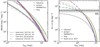 |
Fig. 4. Best-fit number counts models and their integrated energy densities. Left: derived number counts models underlying distribution of sources in ELAN fields compared to blank field models (gray). To highlight the typical uncertainties in these models, we show the confidence bands for the Geach et al. model and for the Jackpot field. Right: extragalactic background light as a function of flux. In both panels, the models for ELANe are plotted in solid at the flux range of the measured counts, and dashed in flux regimes fainter than our measurements. |
As a test, we have tried different radial binning procedures but we found the results insensitive to these choices. There are a few factors that could be the root of the variety in the results compared to the previous work that suggested otherwise. First, there is the sample size. Previous studies have at least twice the number of fields compared to ours and some also have significantly deeper data. This is despite the fact that the observed differences in overdensity between the inner and outer regions reported in these studies are marginal, that is, close to or less than 3 sigma. We therefore expect that our current data quality would not have allowed us to make the detection if the SMGs around ELANe behave similarly to those in other dense fields. Second, while the first factor argues from a purely statistical point of view, it is also possible that the SMGs intrinsically span a wider physical range in the environments around ELANe compared to those around HzRGs or X-ray selected clusters targeted by other studies. The fact that the footprint of our SCUBA-2 observations (Fig. 1) matches the expected span (∼10–20 cMpc) of a protocluster hosting a massive (1013–1014 M⊙) halo at the redshift of our sample ELANe (Chiang et al. 2013) makes the scenario of more widespread SMG distribution around ELANe a plausible hypothesis.
To quantify the overdensity factor for each of the ELANe, we adopted two approaches. In the first approach, which was also adopted in other studies (Arrigoni Battaia et al. 2018b), for each field we first correct the raw counts for observational biases by dividing the raw counts in each flux bin by the ratios of the mean recovered counts to its underlying model obtained from the simulations. We then fit the fiducial model to these corrected counts, allowing only the normalization N0 to vary. The overdensity factor is defined as the ratio of the obtained normalization to fiducial model normalization. As a result, we find that the overdensity factors for each field are 2.7 ± 0.5, 2.0 ± 0.4, 1.8 ± 0.5, 3.8 ± 0.7, respectively. for MAMMOTH-1, the Jackpot, the Slug, and the Fabulous ELANe. The uncertainties in each field have taken into account both Poisson noises and those from the simulations. The weighted average overdensity factor in our sample is 2.3 ± 0.21.
The first approach is appropriate if the shape of the model in ELANe agrees with that of the fiducial model. However, as shown in Fig. 3 and Table 1 there is tentative evidence that the models in ELANe are steeper, so the overdensity could be flux dependent. In such cases, estimating overdensity factors by only fitting the normalization would bias the results to the lower end. To mitigate this bias we therefore estimate the overdensity factors by simply comparing the cumulative number of sources between each ELAN field and the fiducial field. The cumulative number of sources are obtained by integrating the models within the flux range probed by our SCUBA-2 observations (S850 ∼ 2.5 − 10 mJy). As a result, we find overdensity factors of 3.6 ± 0.9, 3.8 ± 1.2, 2.9 ± 1.8, and 3.9 ± 1.5 for MAMMOTH-1, the Jackpot, the Slug, and the Fabulous ELANe, respectively. These give a weighted overdensity factor of 3.6 ± 0.62. As expected, the overdensity factors using the cumulative approach are slightly larger than the normalization approach in the three fields where the best-fit underlying models have slightly steeper slopes. In addition, since the cumulative method additionally includes the uncertainties from the bright-end slope, γ, the uncertainties of the overdensity factors would be larger compared to those of the first approach with fittings only to the normalization. The results from both approaches however are consistent with each other, thus we chose to adopt this second approach since it does not suffer from any possible bias due to the assumptions of the model shape.
Our results are consistent with those found in our pilot study on the MAMMOTH-1 ELAN alone (Arrigoni Battaia et al. 2018a). By expanding the measurements to include three more ELANe, we have found overabundant submillimeter sources around all four ELANe and obtained a more precise average overdensity factor. With these results, we conclude that there are significantly (with a > 4σ confidence level) more SMGs around ELANe in general. We postulate that this overdensity is likely caused by additional SMGs that are physically associated with each ELAN, but future emission line measurements are needed to confirm this hypothesis; this would also allow us to measure the three-dimensional overdensity factors. Our results are also in agreement with submillimeter and millimeter surveys in other samples of AGN, such as high-redshift radio galaxies (HzRGs) and WISE-selected AGN, in which (on average) a factor of 2–6 in overdensity was found (e.g., Rigby et al. 2014; Jones et al. 2017; Zeballos et al. 2018). What we found to be different is that, while it comes with a varying range of significance, the overabundant submillimeter sources is found in all the surveyed ELAN fields; this ubiquity was not observed in other studies where typically less than half of the targeted fields show any signs of overdensity. While surveying more ELAN fields is needed, these findings support the fact that certain levels of co-evolution exist between SMGs and AGN, as they are likely part of similarly dense environments, and the co-evolution may be more commonly observed in the ELAN fields.
On the other hand, if our best-fit count models continue to the fainter end, our findings could have implications for the extragalactic background light (EBL) measurements at 850 μm. In the right panel of Fig. 4, we plot the integrated flux density above a given flux density based on the best-fit models for each ELAN field as well as the fiducial model. By comparing the results to the background light measurements from the COBE satellite (Fixsen et al. 1998), we find that in the ELAN fields, the background light can already be fully accounted for by integrating the counts models down to 1 − 2 mJy, and there would be significantly excessive background light if the models are integrated down to 0.1 mJy level – which is the faintest detection level reported for other fields (e.g., Chen et al. 2014; Fujimoto et al. 2016; Hsu et al. 2017; González-López et al. 2017, 2020). Our results therefore suggest that there could be up to an order of magnitude in fluctuations with regard to the 850 μm background on the survey scales toward these dense fields. On the other hand, if this level of fluctuation does exist, we would expect these extreme fluctuations to be rare; otherwise, a deficit of background light at a similar level would have to exist in some other fields to bring the average down to the observed level by COBE. Deeper observations are key for constructing the shape of the number count distribution at the faint end, which, in turn, will provide better constraints in this area.
Finally, we attempted to estimate the total obscured star formation within the Mpc scale environments of ELAN, which can be achieved by assuming that the excess number of submillimeter sources are all associated with the respective ELAN. To compute the SFR densities we first seek a proper conversion from S850 to SFRs. We utilized a sample of ALMA-identified SMGs in the UKIDSS-UDS field, which has been studied in detail with proper SED fittings (Dudzevičiūtė et al. 2020). Similarly to our observations, the sample of Dudzevičiūtė et al. (2020) was drawn from a flux-limited sample produced by the SCUBA-2 Cosmology Legacy Survey (Geach et al. 2017). Their results should therefore be representative, on average, of SCUBA-2 sources uncovered in other fields. These authors found a linear correlation of log10[SFR(M⊙ yr−1)] = (0.42 ± 0.06) × log10[S870(mJy)] + (2.19 ± 0.03) for their SMGs, which span a flux range of ∼1 − 10 mJy, appropriate for the SCUBA-2 sources discovered in our target ELAN fields. We then computed the total SFR densities by integrating over a given S850 range in which the SFR contribution at a given S850 is the product of the excess number density of the submillimeter sources and their corresponding SFR based on the conversion. For each field, by considering a flux range of S850 = 1 − 20 mJy and assuming a sphere with an equivalent circular radius of the corresponding effective area, we obtain SFR densities of 1100 ± 500, 1100 ± 500, 2300 ± 1100, and 1400 ± 1100 M⊙ yr−1 Mpc−3 for Fabulous, Slug, Jackpot, and MAMMOTH-1 ELAN, and a weighted average SFR density of ΣSFR = 1200 ± 300 M⊙ yr−1 Mpc−3. We plot the results in Fig. 5, showing that they are consistent with those found in the Mpc-scale environments of other quasar samples or proto-clusters at z ∼ 2 − 3 (Clements et al. 2014; Dannerbauer et al. 2014; Kato et al. 2016). This result suggests that the star formation activities around ELANe are at a similar level of other dense systems in this redshift range, or, in other words, at a factor of about 300 greater than the cosmic mean.
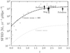 |
Fig. 5. Cosmic SFR density in physical volumes. The estimates based on our counts measurements are plotted in black points, with the corresponding field names indicated. The gray points mark the values reported in the literature around samples of overdense regions (Clements et al. 2014; Kato et al. 2016) that are not known to host ELANe. The cosmic mean is plotted in gray dashed based on Eq. (15) of Madau & Dickinson (2014) but converted to physical volume density, whilst the black curve shows the cosmic mean multiplied by a factor of 300. |
5. Summary
In this second paper of the AMUSE2 series, we present the results of a SCUBA-2 850 μm survey around four ELANe, with the aim of understanding the dust-obscured star formation around these massive systems on Mpc scales. We summarize our findings in the following.
-
By carefully performing the number counts analyses through self-consistent simulations, we find that the number of submillimeter sources with S850 ≳ 3 mJy are overabundant in all four ELANe fields, by a factor of 2–4 within ∼5 Mpc. The significance of overdensity detection in each field varies between 1–4 σ, depending on the precise methods used in computing these overdensity factors. The weighted average overdensity factor is 2.3 ± 0.2, if normalized to the fiducial blank-field counts, or 3.6 ± 0.6, if instead adopting a cumulative method over the flux density range probed.
-
By integrating the number count models in the ELAN fields, we find that the 850 μm EBL would be fully accounted for at 1–2 mJy, and up to an order of magnitude higher when integrating down to about 0.1 mJy; thereby suggesting an order of magnitude fluctuations of the 850 μm EBL on the survey scales toward these dense fields. Deeper observations are key to constraining the count shapes at the faint end, which, in turn, will provide better constraints in this regard.
-
Finally, assuming that all the excessive sources can be attributed to SMGs associated with the corresponding ELANe, and by adopting a linear S850-to-SFR relation reported by a general SMG study (Dudzevičiūtė et al. 2020), we find SFR densities of 1000–2000 M⊙ yr−1 Mpc−3 with a weighted average of ΣSFR = 1200 ± 300 M⊙ yr−1 Mpc−3, which is a factor of about 300 larger than the cosmic mean. These are consistent with those found in other quasar samples or proto-clusters, suggesting that the presence of ELANe in the central ∼100 kpc regions does not significantly affect the dust-obscured star-forming activities on Mpc scales.
This work represents the first step into systematically quantifying the Mpc-scale environments around ELAN from the perspective of dusty star formation. Follow up observations with spectroscopic measurements to confirm member associations would be the next step to understand their spatial and kinematic distributions, key to unlock the formation processes on z ∼ 2 − 3 massive proto-clusters.
If we instead adopt 0.1 mJy as the faintest injected sources for the simulations, the factor would be 2.2 ± 0.3, consistent to within 1σ to the adopted method.
3.5 ± 0.7 if we instead adopt 0.1 mJy as the faintest injected sources for the simulations.
Acknowledgments
We thank the first ever ESO summer research program (Manara et al. 2019) that facilitated the start of this research project; Ian Smail for providing useful comments on this work; and the reviewer for a thoughtful report that has improved the manuscript. C. C. C. acknowledges support from the Ministry of Science and Technology of Taiwan (MOST 109-2112-M-001-016-MY3). M. N. and F. A. B. warmly thank the JCMT staff for their hospitality and support during the observatory visits and observing runs. This project has received funding from the European Research Council (ERC) under the European Union’s Horizon 2020 research and innovation programme (grant agreement No 757535). Y. Y.’s research was supported by Basic Science Research Program through the National Research Foundation of Korea (NRF) funded by the Ministry of Science, ICT & Future Planning (NRF-2019R1A2C4069803). The James Clerk Maxwell Telescope is operated by the East Asian Observatory on behalf of The National Astronomical Observatory of Japan; Academia Sinica Institute of Astronomy and Astrophysics; the Korea Astronomy and Space Science Institute; Center for Astronomical Mega-Science (as well as the National Key R&D Program of China with No. 2017YFA0402700). Additional funding support is provided by the Science and Technology Facilities Council of the United Kingdom and participating universities and organizations in the United Kingdom and Canada. Additional funds for the construction of SCUBA-2 were provided by the Canada Foundation for Innovation. This research made use of Astropy (http://www.astropy.org), a community-developed core Python package for Astronomy (Astropy Collaboration 2013, 2018). The authors wish to recognize and acknowledge the very significant cultural role and reverence that the summit of Maunakea has always had within the indigenous Hawaiian community. We are most fortunate to have the opportunity to conduct observations from this mountain.
References
- An, F. X., Simpson, J. M., Smail, I., et al. 2019, ApJ, 886, 48 [NASA ADS] [CrossRef] [Google Scholar]
- Arrigoni Battaia, F., Hennawi, J. F., Prochaska, J. X., & Cantalupo, S. 2015, ApJ, 809, 163 [NASA ADS] [CrossRef] [Google Scholar]
- Arrigoni Battaia, F., Chen, C.-C., Fumagalli, M., et al. 2018a, A&A, 620, A202 [NASA ADS] [CrossRef] [EDP Sciences] [Google Scholar]
- Arrigoni Battaia, F., Prochaska, J. X., Hennawi, J. F., et al. 2018b, MNRAS, 473, 3907 [NASA ADS] [CrossRef] [Google Scholar]
- Arrigoni Battaia, F., Hennawi, J. F., Prochaska, J. X., et al. 2019, MNRAS, 482, 3162 [NASA ADS] [CrossRef] [Google Scholar]
- Arrigoni Battaia, F., Chen, C.-C., Liu, H. Y. B., et al. 2021, ApJ, submitted [arXiv:2111.15392] [Google Scholar]
- Astropy Collaboration (Price-Whelan, A. M., et al.) 2018, AJ, 156, 123 [Google Scholar]
- Astropy Collaboration (Robitaille, T. P., et al.) 2013, A&A, 558, A33 [NASA ADS] [CrossRef] [EDP Sciences] [Google Scholar]
- Barger, A. J., Cowie, L. L., Sanders, D. B., et al. 1998, Nature, 394, 248 [Google Scholar]
- Barger, A. J., Cowie, L. L., & Richards, E. A. 2000, AJ, 119, 2092 [NASA ADS] [CrossRef] [Google Scholar]
- Barger, A. J., Wang, W. H., Cowie, L. L., et al. 2012, ApJ, 761, 89 [Google Scholar]
- Cai, Z., Fan, X., Yang, Y., et al. 2017, ApJ, 837, 71 [NASA ADS] [CrossRef] [Google Scholar]
- Cai, Z., Cantalupo, S., Prochaska, J. X., et al. 2019, ApJS, 245, 23 [Google Scholar]
- Cantalupo, S., Arrigoni-Battaia, F., Prochaska, J. X., Hennawi, J. F., & Madau, P. 2014, Nature, 506, 63 [Google Scholar]
- Casey, C. M., Chen, C.-C., Cowie, L. L., et al. 2013, MNRAS, 436, 1919 [NASA ADS] [CrossRef] [Google Scholar]
- Chapin, E. L., Berry, D. S., Gibb, A. G., et al. 2013, MNRAS, 430, 2545 [Google Scholar]
- Chapman, S. C., Blain, A. W., Smail, I., & Ivison, R. J. 2005, ApJ, 622, 772 [NASA ADS] [CrossRef] [Google Scholar]
- Chen, C.-C., Cowie, L. L., Barger, A. J., et al. 2013a, ApJ, 762, 81 [NASA ADS] [CrossRef] [Google Scholar]
- Chen, C.-C., Cowie, L. L., Barger, A. J., et al. 2013b, ApJ, 776, 131 [Google Scholar]
- Chen, C.-C., Cowie, L. L., Barger, A. J., Wang, W.-H., & Williams, J. P. 2014, ApJ, 789, 12 [NASA ADS] [CrossRef] [Google Scholar]
- Chen, C.-C., Smail, I., Ivison, R. J., et al. 2016a, ApJ, 820, 82 [NASA ADS] [CrossRef] [Google Scholar]
- Chen, C.-C., Smail, I., Swinbank, A. M., et al. 2016b, ApJ, 831, 91 [NASA ADS] [CrossRef] [Google Scholar]
- Chen, C. C., Arrigoni Battaia, F., Emonts, B., Lehnert, M. D., & Prochaska, J. X. 2021, ApJ, 923, 200 [NASA ADS] [CrossRef] [Google Scholar]
- Chiang, Y. K., Overzier, R., & Gebhardt, K. 2013, ApJ, 779, 127 [NASA ADS] [CrossRef] [Google Scholar]
- Clements, D. L., Braglia, F. G., Hyde, A. K., et al. 2014, MNRAS, 439, 1193 [NASA ADS] [CrossRef] [Google Scholar]
- Cooke, E. A., Smail, I., Stach, S. M., et al. 2019, MNRAS, 486, 3047 [Google Scholar]
- Cowie, L. L., Barger, A. J., Hsu, L. Y., et al. 2017, ApJ, 837, 139 [Google Scholar]
- da Cunha, E., Walter, F., Smail, I. R., et al. 2015, ApJ, 806, 110 [Google Scholar]
- Dannerbauer, H., Kurk, J. D., De Breuck, C., et al. 2014, A&A, 570, A55 [NASA ADS] [CrossRef] [EDP Sciences] [Google Scholar]
- Dempsey, J. T., Friberg, P., Jenness, T., et al. 2013, MNRAS, 430, 2534 [Google Scholar]
- Dudzevičiūtė, U., Smail, I., Swinbank, A. M., et al. 2020, MNRAS, 494, 3828 [Google Scholar]
- Emonts, B. H. C., Cai, Z., Prochaska, J. X., Li, Q., & Lehnert, M. D. 2019, ApJ, 887, 86 [NASA ADS] [CrossRef] [Google Scholar]
- Fixsen, D. J., Dwek, E., Mather, J. C., Bennett, C. L., & Shafer, R. A. 1998, ApJ, 508, 123 [Google Scholar]
- Fujimoto, S., Ouchi, M., Ono, Y., et al. 2016, ApJS, 222, 1 [Google Scholar]
- García-Vergara, C., Hodge, J., Hennawi, J. F., et al. 2020, ApJ, 904, 2 [CrossRef] [Google Scholar]
- Geach, J. E., Dunlop, J. S., Halpern, M., et al. 2017, MNRAS, 465, 1789 [Google Scholar]
- González-López, J., Bauer, F. E., Romero-Cañizales, C., et al. 2017, A&A, 597, A41 [NASA ADS] [CrossRef] [EDP Sciences] [Google Scholar]
- González-López, J., Novak, M., Decarli, R., et al. 2020, ApJ, 897, 91 [Google Scholar]
- Hennawi, J. F., Prochaska, J. X., Cantalupo, S., & Arrigoni-Battaia, F. 2015, Science, 348, 779 [Google Scholar]
- Hickox, R. C., Myers, A. D., Brodwin, M., et al. 2011, ApJ, 731, 117 [NASA ADS] [CrossRef] [Google Scholar]
- Holland, W. S., Bintley, D., Chapin, E. L., et al. 2013, MNRAS, 430, 2513 [Google Scholar]
- Hopkins, P. F., Hernquist, L., Cox, T. J., et al. 2006, ApJS, 163, 1 [Google Scholar]
- Hsu, L.-Y., Cowie, L. L., Barger, A. J., & Wang, W.-H. 2017, ApJ, 850, 189 [NASA ADS] [CrossRef] [Google Scholar]
- Hughes, D. H., Serjeant, S., Dunlop, J., et al. 1998, Nature, 394, 241 [Google Scholar]
- Jenness, T., Cavanagh,, B., Economou, F., & Berry, D. S. 2008, in Astronomical Data Analysis Software and Systems XVII, eds. R. W. Argyle, P. S. Bunclark, & J. R. Lewis, ASP Conf. Ser., 394, 565 [NASA ADS] [Google Scholar]
- Jenness, T., Berry, D., Chapin, E., et al. 2010, in Astronomical Data Analysis Software and Systems XX, eds. I. N. Evans, A. Accomazzi, D. J. Mink, A. H. Rots, et al., ASP Conf. Ser., 442, 281 [NASA ADS] [Google Scholar]
- Jones, S. F., Blain, A. W., Assef, R. J., et al. 2017, MNRAS, 469, 4565 [Google Scholar]
- Kato, Y., Matsuda, Y., Smail, I., et al. 2016, MNRAS, 460, 3861 [Google Scholar]
- Lim, C.-F., Chen, C.-C., Smail, I., et al. 2020, ApJ, 895, 104 [NASA ADS] [CrossRef] [Google Scholar]
- Madau, P., & Dickinson, M. 2014, ARA&A, 52, 415 [Google Scholar]
- Manara, C. F., Harrison, C., Zanella, A., et al. 2019, Messenger, 178, 57 [NASA ADS] [Google Scholar]
- Michałowski, M. J., Dunlop, J. S., Koprowski, M. P., et al. 2017, MNRAS, 469, 492 [Google Scholar]
- Puget, J. L., Abergel, A., Bernard, J. P., et al. 1996, A&A, 308, L5 [Google Scholar]
- Rigby, E. E., Hatch, N. A., Röttgering, H. J. A., et al. 2014, MNRAS, 437, 1882 [NASA ADS] [CrossRef] [Google Scholar]
- Simpson, J. M., Swinbank, A. M., Smail, I., et al. 2014, ApJ, 788, 125 [Google Scholar]
- Smail, I., Ivison, R. J., & Blain, A. W. 1997, ApJ, 490, L5 [NASA ADS] [CrossRef] [Google Scholar]
- Smail, I., Dudzevičiūtė, U., Stach, S. M., et al. 2021, MNRAS, 502, 3426 [NASA ADS] [CrossRef] [Google Scholar]
- Stach, S. M., Smail, I., Swinbank, A. M., et al. 2018, ApJ, 860, 161 [Google Scholar]
- Stevens, J. A., Ivison, R. J., Dunlop, J. S., et al. 2003, Nature, 425, 264 [NASA ADS] [CrossRef] [Google Scholar]
- Swinbank, A. M., Simpson, J. M., Smail, I., et al. 2014, MNRAS, 438, 1267 [Google Scholar]
- Timlin, J. D., Ross, N. P., Richards, G. T., et al. 2018, ApJ, 859, 20 [NASA ADS] [CrossRef] [Google Scholar]
- Toft, S., Smolčić, V., Magnelli, B., et al. 2014, ApJ, 782, 68 [Google Scholar]
- Wang, L., Viero, M., Ross, N. P., et al. 2015, MNRAS, 449, 4476 [NASA ADS] [CrossRef] [Google Scholar]
- Wardlow, J. L., Smail, I., Coppin, K. E. K., et al. 2011, MNRAS, 415, 1479 [Google Scholar]
- White, M., Myers, A. D., Ross, N. P., et al. 2012, MNRAS, 424, 933 [NASA ADS] [CrossRef] [Google Scholar]
- Wilkinson, A., Almaini, O., Chen, C.-C., et al. 2017, MNRAS, 464, 1380 [NASA ADS] [CrossRef] [Google Scholar]
- Zavala, J. A., Aretxaga, I., Geach, J. E., et al. 2017, MNRAS, 464, 3369 [NASA ADS] [CrossRef] [Google Scholar]
- Zeballos, M., Aretxaga, I., Hughes, D. H., et al. 2018, MNRAS, 479, 4577 [Google Scholar]
Appendix A: Source catalogs
In this appendix, we provide the source catalogs for ≥4 σ detection. The last two columns of each table represent the deboosted flux densities ( ) and the positional uncertainties (Δ(α, δ)), which are estimated as follows. We use the 500 simulated maps described in Section 3 in every field to estimate the flux boosting factors and positional uncertainties. In every map, we search for an injected source corresponding to a detected source. An injected source is considered a match if it is located within the beam area of a detected source. We define flux boosting as the ratio of the recovered source flux to the intrinsic source flux. Both flux boosting and positional offsets are recorded for each injected source and we find they are both a function of S/N, which is consistent with previous findings (e.g., Geach et al. 2017). In the catalogs, we therefore apply the median flux boosting correction for each source given its S/N and we quote the corresponding positional uncertainty.
SCUBA-2 850 μm detected sources within the assumed effective area around the Slug ELAN
SCUBA-2 850 μm detected sources within the assumed effective area around the Jackpot ELAN
SCUBA-2 850 μm detected sources within the assumed effective area around the Fabulous ELAN
SCUBA-2 850 μm detected sources within the assumed effective area around the MAMMOTH-1 ELAN
All Tables
Information of the four ELANe in our sample, along with their best-fit parameters for the underlying counts models formulated as Schecter functions.
SCUBA-2 850 μm detected sources within the assumed effective area around the Slug ELAN
SCUBA-2 850 μm detected sources within the assumed effective area around the Jackpot ELAN
SCUBA-2 850 μm detected sources within the assumed effective area around the Fabulous ELAN
SCUBA-2 850 μm detected sources within the assumed effective area around the MAMMOTH-1 ELAN
All Figures
|
Fig. 1. SCUBA-2 signal-to-noise maps at 850 μm for the Fabulous, Jackpot, MAMMOTH-1, and Slug ELANe (yellow star). Sources detected at over 4σ are marked by cyan circles, and the size of the circles represents 2× the FWHM of the beam. The white curve bounds the effective area of every map, which is about 10′ (∼5 Mpc) in diameter. The quasars that contribute significantly to the powering of the corresponding ELAN are marked as yellow stars (coordinates in Table 1). |
| In the text | |
|
Fig. 2. Histogram of signal-to-noise ratio for pixels located within the effective area of the Jackpot map (blue) and the corresponding jackknife map (yellow). The solid vertical line represents the 2.5σ cut used in our simulations. The dashed line represents the threshold of 4σ above which we catalog sources. We note that the excessive negative signals compared to the jackknife map are a result of matched filtering, which can be properly accounted for during source extraction processes using a correct PSF. |
| In the text | |
|
Fig. 3. Differential number counts recovered from 500 realizations of the number counts models determined through Monte Carlo simulations (orange) and the fiducial model (gray). The shaded regions represent the 90% confidence intervals of the counts recovered from the simulated maps. The black points are raw differential number counts, as defined in Sect. 3. The underlying counts models and the fiducial model (Geach et al. 2017) are plotted in blue and gray, respectively. The effect of flux boosting can be observed as the shaded regions are lying above their input model. We note that the lower zero limits of the fiducial model realizations at faint fluxes reflect the non-uniform noise structure of our maps, where incompleteness increases with the distance, from the center of the map. |
| In the text | |
|
Fig. 4. Best-fit number counts models and their integrated energy densities. Left: derived number counts models underlying distribution of sources in ELAN fields compared to blank field models (gray). To highlight the typical uncertainties in these models, we show the confidence bands for the Geach et al. model and for the Jackpot field. Right: extragalactic background light as a function of flux. In both panels, the models for ELANe are plotted in solid at the flux range of the measured counts, and dashed in flux regimes fainter than our measurements. |
| In the text | |
|
Fig. 5. Cosmic SFR density in physical volumes. The estimates based on our counts measurements are plotted in black points, with the corresponding field names indicated. The gray points mark the values reported in the literature around samples of overdense regions (Clements et al. 2014; Kato et al. 2016) that are not known to host ELANe. The cosmic mean is plotted in gray dashed based on Eq. (15) of Madau & Dickinson (2014) but converted to physical volume density, whilst the black curve shows the cosmic mean multiplied by a factor of 300. |
| In the text | |
Current usage metrics show cumulative count of Article Views (full-text article views including HTML views, PDF and ePub downloads, according to the available data) and Abstracts Views on Vision4Press platform.
Data correspond to usage on the plateform after 2015. The current usage metrics is available 48-96 hours after online publication and is updated daily on week days.
Initial download of the metrics may take a while.