| Issue |
A&A
Volume 658, February 2022
|
|
|---|---|---|
| Article Number | A132 | |
| Number of page(s) | 18 | |
| Section | Planets and planetary systems | |
| DOI | https://doi.org/10.1051/0004-6361/202039037 | |
| Published online | 10 February 2022 | |
Probing Kepler’s hottest small planets via homogeneous search and analysis of optical secondary eclipses and phase variations
1
Dip. di Fisica e Astronomia “Ettore Majorana”, Università di Catania,
Via S.Sofia 64,
95123,
Catania,
Italy
2
INAF – Osservatorio Astrofisico di Catania,
Via S.Sofia 78,
95123,
Catania,
Italy
e-mail: This email address is being protected from spambots. You need JavaScript enabled to view it.
3
INAF – Osservatorio Astrofisico di Torino,
Via Osservatorio, 20,
10025
Pino Torinese,
TO,
Italy
4
Dipartimento di Fisica, Università degli Studi di Torino,
via Pietro Giuria 1,
10125
Torino,
Italy
5
Observatoire de Genève, Université de Genève,
51 Chemin des Maillettes,
1290
Sauverny,
Switzerland
6
Space Research Institute, Austrian Academy of Sciences,
Schmiedlstr. 6,
8042
Graz,
Austria
Received:
27
July
2020
Accepted:
8
November
2021
Abstract
Context. High-precision photometry can lead to the detection of secondary eclipses and phase variations of highly irradiated planets.
Aims. We performed a homogeneous search and analysis of optical occultations and phase variations of the most favorable ultra-short-period (USP) (P < 1 days) sub-Neptunes (Rp < 4 R⊕), observed by Kepler and K2, with the aim to better understand their nature.
Methods. We first selected 16 Kepler and K2 USP sub-Neptunes based on the expected occultation signal. We filtered out stellar variability in the Kepler light curves, using a sliding linear fitting and, when required, a more sophisticated approach based on a Gaussian process regression. In the case of the detection of secondary eclipse or phase variation with a confidence level higher than 2σ, we simultaneously modeled the primary transit, secondary eclipse, and phase variations in a Bayesian framework, by using information from previous studies and knowledge of the Gaia parallaxes. We further derived constraints on the geometric albedo as a function of the planet’s brightness temperature.
Results. We confirm the optical secondary eclipses for Kepler-10b (13σ), Kepler-78b (9.5σ), and K2-141b (6.9σ), with marginal evidence for K2-312b (2.2σ). We report new detections for K2-106b (3.3σ), K2-131b (3.2σ), Kepler-407b (3.0σ), and hints for K2-229b (2.5σ). For all targets, with the exception of K2-229b and K2-312b, we also find phase curve variations with a confidence level higher than 2σ.
Conclusions. Two USP planets, namely Kepler-10b and Kepler-78b, show non-negligible nightside emission. This questions the scenario of magma-ocean worlds with inefficient heat redistribution to the nightside for both planets. Due to the youth of the Kepler-78 system and the small planetary orbital separation, the planet may still retain a collisional secondary atmosphere capable of conducting heat from the day to the nightside. Instead, the presence of an outgassing magma ocean on the dayside and the low high-energy irradiation of the old host star may have enabled Kepler-10b to build up and retain a recently formed collisional secondary atmosphere. The magma-world scenario may instead apply to K2-141b and K2-131b.
Key words: planets and satellites: terrestrial planets / planets and satellites: atmospheres / planets and satellites: surfaces / techniques: photometric
© ESO 2022
1 Introduction
Ultra-short-period (USP, P < 1 days) sub-Neptunes (Rp < 4 R⊕) are intriguing planets because of the very close proximity to their host stars. They are about as common as hot Jupiters (Winn et al. 2018) and are often members of multi-planet systems (Sanchis-Ojeda et al. 2014). The existence of USP sub-Neptunes is not easily explained by current formation and migration models (Carrera et al. 2018), although it is generally believed that they migrated from outer regions. Indeed, their formation is highly improbable at the present location because of temperatures higher than the dust sublimation radius (a∕R⋆ ~ 8 for Sun-like stars; e.g., Isella et al. 2006).
So far, a small number of USP planets have been well characterized thanks to space-based photometry and high-precision radial-velocity follow-up studies, such as Corot-7b (Léger et al. 2011; Haywood et al. 2014), Kepler-10b (Batalha et al. 2011; Dumusque et al. 2014; Weiss et al. 2016), Kepler-78b (Sanchis-Ojeda et al. 2013; Pepe et al. 2013; Howard et al. 2013), K2-141b (Malavolta et al. 2018; Barragán et al. 2018), 55 Cancrie (Demory et al. 2016a; Nelson et al. 2014), K2-229b (Santerne et al. 2018), WASP-47e (Weiss et al. 2017; Vanderburg et al. 2017), K2-131b (Dai et al. 2017), K2-106b (Sinukoff et al. 2017; Guenther et al. 2017), and K2-312b (Frustagli et al. 2020). Most USP small planets have a rocky compositionwith varying silicate-to-iron mass fractions (Dai et al. 2019) and are generally less massive than 8 M⊕. Some of them could be the remnant cores of hot Neptunes or sub-Saturns that lost their primordial H or He atmospheres under the action of the intense stellar irradiation, particularly, while the star was still young and, hence, active (photo-evaporation) (Lecavelier Des Etangs 2007; Winn et al. 2017; Kubyshkina et al. 2018). Depending on the planet’s surface gravity and on the timescale and strength of the competing photo-evaporation and surface outgassing or release processes, USP planets may or may not possess an atmospheric envelope (Miguel et al. 2011; Lopez & Fortney 2013; Owen & Wu 2017; Ito et al. 2015; Kislyakova & Noack 2020). Only a collisional atmosphere, with a relatively high molecular weight in the case of USP planets, may be able to retain and redistribute heat, as might be the case of 55 Cnc e (Dawson & Fabrycky 2010; Winn et al. 2011; Demory et al. 2011, 2016b; Dai et al. 2019).
The surface of rocky USP planets may be at least partially covered by magma because, at their equilibrium temperatures (typically higher than ~2200 K), silicates melt (Schaefer & Fegley 2004, 2009; Schaefer et al. 2012). In this scenario of “magma-ocean worlds,” a very high temperaturecontrast is expected between the continuously illuminated dayside of the planet and its hidden nightside. Indeed, any possible non-collisional atmosphere (i.e., exosphere) of metal vapors above the magma surface would be unable to transfer heat to the nightside (Léger et al. 2011). As a result, the nightside flux of a magma-ocean world is expected to be negligible.
The observation of transiting systems from space-based high-precision photometry as provided by the optical Kepler Space Telescope allows us to detect secondary eclipses and phase variations (Esteves et al. 2013, 2015; Sheets & Deming 2017; Jansen & Kipping 2018), especially when a large number of orbital phases can be combined as in the case of USP planets. The secondary eclipse depth is a measure of the brightness of the planet and, in the optical band, results from two contributions: the reflection of stellar light from the planetary atmosphere and the planet thermal emission. The latter may in principle be the dominant contribution for USP sub-Neptunes, given the very high irradiation these planets receive from their host stars. With optical data only, it is not possible to disentangle the reflected and thermal contributions (Cowan & Agol 2011). Nevertheless, non-negligible nightside flux – as derived from the difference between the occultation depth and the flux level just before (after) the transit ingress (egress) – can only be due to thermal nightside emission and, hence, indicate the presence of either a mechanism capable of heating the planetary nightside surface or of heat redistribution from the dayside to the nightside.
In this work, we present a homogeneous search for and analysis of secondary eclipses and phase variations in Kepler and K2 USP sub-Neptunes, with the precise aim of better understanding the nature of these planets.
2 Target selection
The USP sub-Neptunes considered in our study were selected from the Kepler and K2 catalogs of confirmed planets with P < 1 days, Rp < 4 R⊕ and a Kepler magnitude of the host star < 14. The data were collected from the NASA Exoplanet Archive1. Kepler is the most precise space-based telescope to date, both in terms of its exquisite photometric precision and the length of photometric datasets (stellar light curves).
Given the size and distance of the USP planets from their host star, a secondary eclipse can be observed if the signal-to-noise ratio (S/N) is high enough to enable the detection of a flux decrease of at least a few ppm, when the planet passes behind its host star. For each selected USP planet, we computed the expected S/N for the secondary eclipse as:
 (1)
(1)
where σ is the photometric precision of the Kepler light curve, which is related to the brightness of the host star in the Kepler band-pass; Nep is the number of data points during all observed eclipses: the larger the number of planetary orbits observed by Kepler, the higher Nep and, thus, the S/N of the occultation. δec is the estimated depth of the secondary eclipse that was computed with Eqs. (9), (10), and (11) (Sect. 4.4) by (i) using the stellar and planetary parameters from previous studies; and (ii) considering a conservative Bond albedo of AB = 0.5 under the assumption of isotropic scattering by a perfect Lambertian sphere, namely, Ag = 2∕3 ⋅ AB (Rowe et al. 2006), and no heat redistribution to the nightside (Eq. (18) in Sect. 4.6 for ϵ = 0).
We selected only those targets with theoretically computed S∕N ≥ 2 on the secondary eclipse depth (Eq. (1)). The USP planets that meet this criterion are Kepler-10b, Kepler-78b, Kepler-407b, Kepler-1171b, and Kepler-1323b among the Kepler planets, and K2-23e/WASP-47e, K2-96b/HD 3167b, K2-100b, K2-106b, K2-131b, K2-141b, K2-157b, K2-183b, K2-229b, K2-266b, and K2-312b/HD 80653b from the K2 confirmed planets. However, after the analysis of the Kepler and K2 light curves, only eight USP sub-Neptunes: mainly Super-Earths, namely, Kepler-10b, Kepler-78b, Kepler-407b, K2-106b, K2-131b, K2-141b, K2-229b, and K2-312b, are found to show optical secondary eclipses with S∕N > 2 (see Sect. 5).
3 Stellar parameters
With the availability of DR2 Gaia parallaxes (Gaia Collaboration 2018), we improved the parameters of the stellar hosts of the above-mentioned eight systems with secondary eclipses detected at S∕N > 2, to impose a prior on the stellar density (Winn 2010) in the global modeling of transits, secondary eclipses, and phase variations (see Sect. 4.2). We re-determined the radius and mass of the host stars by fitting the stellar Spectral Energy Distribution (SED) and using the MESA Isochrones and Stellar Tracks (MIST; Dotter 2016; Choi et al. 2016) with the publicly available EXOFASTv2 code (Eastman et al. 2019), which makes use of the differential evolution Markov chain Monte Carlo (DE-MCMC, Ter Braak 2006) Bayesian technique. The stellar parameters were simultaneously constrained by the SED and the MIST isochrones, as the SED primarily constrains the stellar radius R* and effective temperature Teff, and a penalty for straying from the MIST evolutionary tracks ensures that the resulting star is physical in nature.
For each star, we fitted the available archival magnitudes from the WISE bands (Cutri & et al. 2014), Sloan bands from the APASS DR9 (Henden et al. 2015), Johnson’s B, V, R and 2MASS J, H, K bands from the UCAC4 catalog (Zacharias et al. 2012), the Kepler (Greiss et al. 2012) and Gaia (Gaia Collaboration 2018) bands. We imposed Gaussian priors on the Gaia DR2 parallax as well as on the stellar effective temperature Teff and metallicity [Fe/H] from the literature values. The DR2 parallax value was first corrected for the systematic offset of 82 ± 33μas as reported in Stassun & Torres (2018). The prior on the parallax greatly helps constraining the stellar radius and in general improves the accuracy and precision of the stellar parameters. In Table 1, we present the improved parameters of the stars hosting the planets for which we found the secondary eclipse at S∕N > 2. For Kepler-10, we used the very precise stellar density as computed through asteroseismology (Fogtmann-Schulz et al. 2014). Along with it, we obtained the mass, radius, luminosity, and age from the same source. The stellar density determination was later used as a prior in the simultaneous fit of the transit, secondary eclipse, and phase variation (see Sect. 4.2).
Stellar parameters from the SED fitting and the MIST evolutionary tracks (Eastman et al. 2019).
4 Light curve analysis
For the selected Kepler targets (Sect. 2), we downloaded the Kepler light curves, both in long-cadence (29.4 min) and short-cadence (58 s) sampling (when available), from the Kepler Mikulski Archive for Space Telescopes (MAST)2. For the K2 targets, we used the light curves extracted and calibrated by Vanderburg & Johnson (2014) and Vanderburg et al. (2016). The light curves were corrected for possible contamination of background stars as reported in the Kepler Input Catalogue (Brown et al. 2011).
4.1 Search for secondary eclipses and phase variations
From the downloaded light curves we removed possible stellar variability due to the rotational modulation of photospheric active regions, following the method described by Sanchis-Ojeda et al. (2013). This is basically a sliding linear fitting (SLF) over the out of primary transit and secondary eclipse data points with a timescale equal to the orbital period (cf. Sect. 3.2 in Sanchis-Ojeda et al. 2013 for more details). Since the orbital period of USP planets is considerably shorter than typical stellar rotation signals (Prot ≳ 10 days), in most cases, this method efficiently filters out stellar variations, while preserving in particular the planet phase variations (as an example, see its application to K2-141 in Fig. 1). Indeed, it has enabled the discovery of the secondary eclipse and phase variations of Kepler-78b and K2-141b orbiting active stars (Sanchis-Ojeda et al. 2013; Malavolta et al. 2018). In the case of a multiple transiting system, the transits of the planetary companions were removed before the filtering of stellar variability. We then phase-folded the detrended light curves for a visual inspection of the secondary eclipse and phase variations. The targets showing a clear signal of a secondary eclipse or a hint of it were further studied in a Bayesian framework through DE-MCMC analyses (Ter Braak 2006) of the detrended light curves.
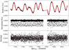 |
Fig. 1 Detrending of the stellar variability in the light curve of K2-141 using the sliding linear fitting. Top: K2-141 light curve after removing the transits of planet c; the SLF model is over-plotted in red. Middle: detrended light curve. Bottom: residual of the model with the best-fit planetary parameters. |
4.2 Model and analysis of transits, secondary eclipses and phase curves
We define the model used for the DE-MCMC analyses as a combination of a transit model, a phase curve, and a secondary eclipse model, following Esteves et al. (2013) as follows:
 (2)
(2)
Ftr is the transit model with the formalism of Mandel & Agol (2002) for a quadratic limb-darkened law. The term for phase variations Fph is defined as (Perryman 2011, and references therein):
 (3)
(3)
where Aph is the phase amplitude, α ∈ [0, π] is the angle between the star and the observer subtended at the planet with cos α = − sin(i)sin(2π(ϕ(t) + 0.25)), i ∈ [0, π∕2], and ϕ being the orbital inclination and the orbital phase, respectively, with ϕ = 0 at mid-transit. The angle (ϕ + 0.25) corresponds to the position at radial velocity maximum for a circular orbit (quadrature). The phase function is truncated near its peak at ϕ = 0.5 for the entire duration of the secondary eclipse because the full illuminated planet disk is occulted by the star.
The function of the secondary eclipse Fec is made up of three parts: (i) the out of secondary eclipse flux which is set to zero; (ii) the flux at the eclipse ingress and egress which is derived by calculating the area of the planet being occulted by the star during ingress and egress; and (iii) the complete occultation part with depth δec. The area of the unocculted planetary disk visible to the observer Aec can thus be computed as
 (4)
(4)
where p is the planet’s radius and ζ(t) is the projected distance between the stellar and the planetary disk centers, both in unit of stellar radius; α1 and α2 are the cosine angles given by:
 (5)
(5)
Then, Fec is then defined as:
 (6)
(6)
The orbits of USP planets are expected to be tidally locked and, hence, circular and co-rotational because of the very strong tidal effects at the extreme proximity to their host star. By considering circular orbits, the free parameters of our model are the orbital period (P), the epoch of mid-transit (Tc), the transit duration (Tdur), the orbital inclination (i), the planet-to-stellar radius ratio (p), the eclipse depth(δec), and the amplitude of phase variation (Aph). A phase offset term was also explored, but it was found to be consistent with zero in the phase curves with the highest precision (Kepler-10b and Kepler-78b; see Fig. A.9 for Kepler-10b) and was therefore fixed to zero in our model. We included an additional term ϵref to F(t) in Eq. (2) because even though our light curves were normalized to 1 in relative flux by the sliding linear fitting (Sect. 4.1), this term allows for possible, albeit very small, changes in the reference level of the out-of-transit flux. The limb-darkening coefficients were fixed to the theoretically computed values for the stellar effective temperature, surface gravity, and metallicity (Sing 2010). To derive more accurate and precise transit parameters, we imposed a prior on the stellar density using the values in Table 1 (Sect. 3). This prior affects all the transit parameters except Tc and, at the same time, speeds up the DE-MCMC analyses. The stellar density is indeed related to the other parameters through the relation:
 (7)
(7)
where
 (8)
(8)
and θ1 = − Tdur∕(2P) is the orbital phase at the transit ingress (Giménez 2006).
For the analysis of the Kepler long-cadence data, the model was oversampled at 1 min sampling and then binned to the long-cadence samples to overcome the well-known issue of light-curve distortions due to long integration times (Kipping 2010). For the DE-MCMC analyses, we used a Gaussian likelihood function and the Metropolis-Hastings algorithm to accept or reject a proposal step. We followed the prescriptions given by Eastman et al. (2013, 2019) about the number of DE-MCMC chains (16, specifically, twice the number of free parameters) and the criteria for the removal of burn-in points and the convergence and proper mixing of the chains. The chains were initialized close to the literature values for the transit parameters and relatively close to the expected theoretical values for δec and Aph. The median values and the 15.86–84.13% quantiles of the obtained posterior distributions were respectively taken as the best-fit values and 1σ uncertainties for each fitted parameter.
4.3 Modeling with Gaussian processes
For most of the targets, the SLF technique described in Sect. 4.1 performed well in terms of removing stellar variability by leaving practically negligible correlated noise in the residuals (≲ 15% relative to the photometric rms), as estimated following Pont et al. (2006) and Bonomo et al. (2012). However, in two cases of particularly active stars, namely K2-131 and K2-229, a significantly higher correlated noise was still present after the SLF filtering, that is, 32% and 43% of the residual rms, respectively. This indicates that the SLF was unable to account for short-term activity variations of these two stars and, thus, a more sophisticated approach is needed.
As the correlated noise is expected to be a consequence of active regions co-rotating with the stellar surface, we employed a Gaussian process (GP) regression with a Simple Harmonic Oscillator covariance kernel (Foreman-Mackey et al. 2017). We thus modeled theunfiltered light curve simultaneously with the GP regression and the planetary model (Eq. (2)). We used the celerite2 package (Foreman-Mackey et al. 2017; Foreman-Mackey 2018) for the GP implementation. The posterior samples of the free parameters were derived with an MCMC method, using the emcee package (Foreman-Mackey et al. 2013)3. The results of the GP hyper-parameters, namely the GP amplitude, the damping time scale and the undamped period, are given in Table 2; the corresponding transit, secondary eclipse, and phase curve parameters of K2-131b and K2-229b are presented inSect. 5. The residuals of the best fit of the light curves of K2-131 (in Fig. 2) and K2-229 (in Fig. B.2) show no significant correlated noise, proving that for these two cases the GP approach performed better than the SLF.
Considering the GP modeling being computationally demanding and time consuming due to the large number of photometric data points, we employed the SLF filtering for all the targets but K2-131 and K2-229, as the leftover correlated noise in the SLF residuals is insignificant. Nonetheless, we compared the results of the two approaches, SLF vs GP, for K2-141 and obtained fully consistent results (Table 3). This points to a similar efficiency of the techniques when the residuals of the SLF do not show high correlated noise.
Best-fit Gaussian process hyper-parameters for the three systems when applied.
Comparison of the transit, secondary eclipse and the phase curve model parameters of K2-141b with two different detrending techniques, namely the sliding linear fitting and Gaussian processes.
4.4 Secondary eclipses and constraints on dayside reflection and thermal emission
The optical dayside flux from the secondary eclipse depth is a combination of the reflected light and thermal emission from the planet (e.g., López-Morales & Seager 2007; Snellen et al. 2009):
 (9)
(9)
where δref is the reflected flux and δtherm represents the dayside thermal emission. The two components can be expressed as:
 (10)
(10)
![Mathematical equation: \begin{equation*}\delta_{\textrm{therm}}\,{=}\,\pi\left(\frac{R_{\textrm{p}}}{R_{\star}}\right){}^{2} \frac{\int_{\lambda} \frac{2hc^{2}}{\lambda^{5}} \left[\textrm{exp} \left(\frac{hc}{k_{\textrm{B}}\lambda T_{\textrm{d}}}\right) - 1 \right]^{-1} \Omega_{\lambda} \textrm{d}\lambda}{\int_{\lambda} S_{\lambda}^{CK} \Omega_{\lambda} \textrm{d}\lambda},\end{equation*}](/articles/aa/full_html/2022/02/aa39037-20/aa39037-20-eq11.png) (11)
(11)
where Ag is the geometric albedo, a the semi-major axis, h is the Planck constant, kB the Boltzmann constant, c the speed of light, Td the planet’s dayside brightness temperature. and  is the stellar flux as computed by Castelli & Kurucz (2003) for the stellar Teff, log g, and [Fe/H]; both the planetary and stellar flux are integrated over the Kepler passband Ωλ 4. In addition, Rp∕a is derived from the model fit following Eq. (12) in Giménez (2006).
In order to estimate the relative fraction of reflection and thermal emission from the occultation depth, Eqs. (9), (10), and (11) are used to compute the geometric albedo as a function of varying dayside brightness temperature.
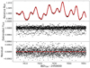 |
Fig. 2 Gaussian-process detrending of the stellar variability in the light curve of K2-131. Top: light curve with the GP model over-plotted in red. Middle: detrended light curve. Bottom: best-fit residuals of the combined fit. The GP detrending and model fitting are carried out simultaneously, unlike the SLF detrending. |
4.5 Phase variations and constraints on the nightside emission
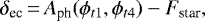
The phase curve conveys information about the flux from the planet dayside as the planet moves along its orbit. The difference between the eclipse depth δec and the amplitude of the phase variation Aph allows us to estimate the nightside flux. Indeed, the flux during the secondary eclipse corresponds to the stellar flux only because the planet is hidden by the star. The flux at the base of the phase curve just before or after transit (phases T1 ∕T4 respectively in Fig. 3) instead includes the possible contribution from the nightside thermal emission, as well as the flux  due to the reflection and thermal emission of the thin bright crescent of the illuminated planet hemisphere. On the other side, just before and after the conjunction (phases t1∕t4), the dayside hemisphere is not entirely visible because a small fraction of it, say
  , is hidden from the observer (it is equal in area to the dark crescent that is in view at this epoch). Therefore,
  can be computed as the difference between the maximum of the phase variation at phase 0.5 and the value of the phase curve at the secondary eclipse ingress t1 or egress t4 as (see Fig. 3)
 (12)
(12)
where  is the phase curve value computed at t1 or t4. The difference between the flux level
  at the transit ingress (egress) T1∕T4 and the bottom of the secondary eclipse, that is, the flux from the star alone (Fstar), has two contributions: (i) the nightside emission δnight and (ii) the reflection and emission from the crescent of the illuminated hemisphere
  . Therefore, as shown in Fig. 3, we can compute the nightside flux δnight5 from the following set of equations:
 (13)
(13)
 (14)
(14)
 (15)
(15)
and, based on symmetry considerations, the bright crescent at T1 ∕T4 will be exactly equal in area to the crescent of the illuminated hemisphere, which is directed away from the observer just before and after occultation, that is, at t1/t4. In other words:
 (16)
(16)
 (17)
(17)
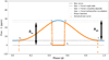 |
Fig. 3 Phase curve of a circular orbit around the secondary eclipse showing the difference flux reference levels. The duration of the secondary eclipse is equal to the transit duration. The times t1, t2, t3, and t4 define the ingress and egress moments of the planetary occultation in the same way as T1, T2, T3, T4 for the primary transit. The eclipse depth is actually the difference between the flux references of planet’s brightness at t1 ∕t4 and the stellar brightness at t2∕t3. |
4.6 Dayside and nightside temperatures
After estimating δnight with Eq. (17), nightside temperatures could, in principle, be derived from Eq. (11) by replacing δtherm with δnight and Td with Tn. The theoretical dayside and nightside effective temperatures, following Cowan & Agol (2011), are equal to:
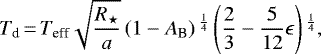 (18)
(18)
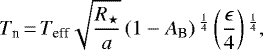 (19)
(19)
where AB is the Bond albedo and ϵ is the heat circulation efficiency that parameterizes the heat flow from the dayside to the nightside: ϵ = 0 indicates no heat circulation to the nightside, while ϵ = 1 means perfect heat redistribution. Assuming a zero Bond albedo, that is, a perfectly absorbing exoplanet, the maximum dayside temperature is equal to  , which corresponds to ϵ = 0 and thus Tn = 0 K; the lower limit would be the uniform temperature for ϵ = 1, namely:
  .
.
The maximum value of Ag for 100% reflection and a null thermal emission (δec = δref) further permits us to estimate the maximum possible Bond albedo AB by using the relation AB = 3∕2 Ag for a perfect Lambertian sphere (Rowe et al. 2006). In this way, the lower limit on Td corresponding to the maximum AB value and ϵ = 1 can be computed. However, this relation cannot be assumed when Ag itself is closeto or greater than 1. Moreover, in the case of significant nightside emission, we can further constrain the lower limit on Td as Td ≥ Tn, because the dayside cannot be colder than the nightside (ϵ = 1).
5 Results
We searched for the secondary eclipse and phase variations for each of the 16 USP planets that successfully passed our selection criterion described in Sect. 2. However, we detected the secondary eclipse with S∕N > 2 only in half of our sample, that is, in the eight systems Kepler-10b, Kepler-78b, Kepler-407b, K2-106b, K2-131b, K2-141b, K2-229b, and K2-312b, which are discussed sequentially below. The secondary eclipse and phase variations went undetected in the other systems mainly because the signal of the optical occultation is actually shallower than our conservative estimates in Sect. 2 and, thus, is buried in the noise.
5.1 Kepler-10b
Kepler-10b is the first rocky planet discovered by the Kepler space telescope in 2011 (Batalha et al. 2011). It orbits a ~10 Gyr-old solar-like G dwarf with a period of 0.837 d or ~20 hrs, and has a transiting companion with a period of ~ 45 d (Fressin et al. 2011; Dumusque et al. 2014; Weiss et al. 2016). The planet’s mass is around 3.6 M⊕ and a radius of 1.48 R⊕. From its bulk density, interior structure models suggest a rocky, Earth-like composition. The best-fit model parameters of our simultaneous fit of transit, secondary eclipse, and phase curve to the Kepler short-cadence data are listed in Table 4 and the best-fit model plot is shown in Fig. 4.
The secondary eclipse depth is found to be 10.4 ± 0.9 ppm and theamplitude of the phase variation 7.4 ± 0.8 ppm. The difference between these two parameters indicates a nightside emission of 3.0 ± 1.2 ppm (Eq. (17)), which is significant at the 2.5σ level. This fully agrees with the results of Fogtmann-Schulz et al. (2014), but is slightly at odds with other works reporting negligible nightside emission (Sheets & Deming 2014; Hu et al. 2015; Esteves et al. 2015). The nightside temperature corresponding to our nightside emission is Tn ~ 2800 K. The temperature of the dayside cannot be lower than Tn and must be, thus, Td ≥ 2800 K.
From δec, we computed the geometric albedo as a function of the dayside temperature (using Eqs. (10) and (11)). The Ag vs Td plot is shown in Fig. 5. The maximum Ag value corresponds to a relatively high value of 0.74 ± 0.06, but Ag should be lower than ~ 0.6 from the previous estimate on the dayside temperature of Td ≥ 2800 K (Fig. 5). On the contrary, the maximum dayside temperature for a perfectly absorbing planet (Ag = 0) is  K (see Fig. 5 for zero fractional reflected light). The two theoretical dayside temperatures, namely
  and
and  (see Sect. 4.6), are also shown in the plot.
Best-fit parameters and associated uncertainties from our fit of primary transits, secondary eclipses, and phase variations.
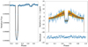 |
Fig. 4 Planetary light curve showing the primary transit, secondary eclipse and the phase variation. Left: detrended, phase-folded, and binned light curve of Kepler-10b (blue points). The best-fit model is over-plotted in solid black line. Right: enlarged view of the secondary eclipse and phase variation. Uncertainties of the best-fit model are shown at 1σ and 3σ in dark and light orange, respectively. The residuals of the best-fit model are displayed in the bottom. |
5.2 Kepler-78b
Kepler-78b is a rocky super-Earth orbiting a relatively young G-type dwarf with an age of ~750 Myr old in an 8.5 h orbit (Sanchis-Ojeda et al. 2013; Howard et al. 2013; Pepe et al. 2013). The planet has a mass of 1.8 M⊕ and a radius of 1.2 R⊕ resulting in an Earth-like density of 5.3 g cc−1. Short-cadence data for this target is not available and therefore we used the 4-yr long-cadence light curve for our analysis. Our best-fit model is shown in Fig. 6.
Our analysis shows a high-confidence secondary eclipse detection with δec = 12.4 ± 1.3 ppm and a phase-amplitude of 7.6 ± 1.0 ppm and, hence, similar to Kepler-10b, the difference implies a nightside emission of δnight = 4.8 ± 1.6 ppm (3σ). Compared to the results of Sanchis-Ojeda et al. (2013), that is, δec = 10.5 ± 1.2 ppm and Aph = 8.8 ± 1.0 ppm, we obtained a slightly deeper secondary eclipse and a slightly lower amplitude of phase variation, although our solution and theirs agree within 2σ. The nightside emission corresponds to a temperatureTn ~ 2700 K and, hence, it gives a lower limit to the dayside temperature, Td ≳ 2700 K). The relationbetween Ag and Td for the measured δec is shown in Fig. 7; Ag tends to 0.48 ± 0.06 at the saturation level, that is, for the lower dayside temperatures, while the maximum dayside temperature for a null reflection (Ag = 0) is 3060 K. Using the lower limit on the dayside temperature, we further constrain the geometric albedo to be less than 0.3.
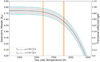 |
Fig. 5 Geometric albedo (Ag) estimated as a function of the dayside temperature of Kepler-10b. The cyan lines correspond to the 3σ uncertainty in the computation of Ag. The two vertical red lines and orange regions display the theoretical temperatures and associated 1σ error bars, by considering zero Bond albedo and negligible or perfect heat redistribution. The maximum geometric albedo is at 0.74 ± 0.06. The maximum dayside temperature can be as high as 3430(+50∕−40) K in the case of100% thermal emission. |
5.3 Kepler-407b
Kepler-407b orbits a G dwarf in a 16 hr period. Previous RV analysis on this target provided an upper limit on the planet’s mass and also a partial orbit of a non-transiting companion (Marcy et al. 2014). We determined its radius precisely at 1.07 ± 0.02R⊕. Furthermore, we present a 3σ detection of a secondary eclipse depth at 6 ± 2 ppm and a phase variation with an amplitude at 3.2 ± 1.5 ppm. The difference of these two parameters is positive, but not precise enough to claim evidence for a significant nightside emission. The best-fit model plot is shown in Fig. 8.
Using the secondary eclipse depth value, we computed Ag as a function of Td (see Fig. 9). The maximum geometric albedo, in the case where the eclipse depth is due to the pure reflection of the stellar light, is 0.56 ± 0.19. By assuming isotropic scattering from the planet, that is, AB = 3∕2Ag, we obtained lower limits on thedayside temperature as Td ≥ 1400 K and Td ≥ 1800 K for ϵ = 1 and ϵ = 0, respectively.In the case of pure thermal emission, the dayside temperature could be as high as 3270 ± 140 K.
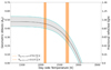 |
Fig. 7 Constraints on the geometric albedo and the dayside temperature of Kepler-78b (ref. Fig. 5). The maximum geometric albedo is 0.48 ± 0.06. The maximum dayside temperature is 3060(+40∕−50) K in the case of100% thermal emission. |
5.4 K2-141b
K2-141b is a rocky super-Earth in a 6.7 h orbit around an active K-dwarf with a rotation period of ~14 days (Malavolta et al. 2018; Barragán et al. 2018). The planet has a mass of 5.1 M⊕ (Malavolta et al. 2018) and a radius of 1.5 R⊕, thereby resulting in a super-terrestrial density of 8.2 g cc−1. Our analysis provides a robust detection (> 6σ) of both the eclipse depth at 26.2 ppm and the phase variation with an amplitude of 23.4
 ppm, in agreement with Malavolta et al. (2018). Since δec and Aph are indistinguishable within the error bars, there is no indication of thermal emission from the nightside. Figure 10 shows the phase-folded transit, eclipse, and phase variation along with the best-fit model.
Given the observed eclipse depth (δec), we computed Ag as a function of Td (Fig. 11). The geometric albedo saturates at 0.34 ± 0.05. Assuming isotropic scattering for Ag = 0.34, we obtain an upper limit of 0.5 on the Bond albedo and, therefore, the theoretical lower limit on the dayside temperature is computed to be ~2300 K for ϵ = 0. The maximum dayside temperature that the planet could achieve for no reflection is  K.
K.
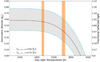 |
Fig. 9 Constraints on the geometric albedo and the dayside temperature of Kepler-407b (ref. Fig. 5). The geometric albedo at saturation is 0.56(+0.19∕−0.18), while the maximum dayside temperature is 3270 ± 140 K. |
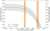 |
Fig. 11 Constraints on the geometric albedo and the dayside temperature of K2-141b (ref. Fig. 5). The maximum geometric albedo is 0.34 ± 0.05, while the maximum dayside temperature is 2860(+50∕−60) K. |
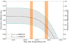 |
Fig. 13 Constraints on the geometric albedo and the dayside temperature of K2-131b (ref. Fig. 5). The maximum geometric albedo is 0.55(+0.18∕−0.17), while the maximum dayside temperature is 3320(+140∕−180) K. |
5.5 K2-131b
The K2-131 system consists of a single discovered exoplanet in an 8.86 hr orbit around an active late G main-sequence star with a rotation period of ~11 days (Dai et al. 2017). The planet’smass of 6.3 M⊕ (Dai et al. 2019)and a radius of 1.6 R⊕ results in a similar composition as that of K2-141b. The simultaneous model of transit, eclipse, and phase variation corresponding to the best-fit parameters is shown in Fig. 12.
With a confidence level slightly higher than 3σ, we found a secondary eclipse depth of  ppm and an amplitude of the phase variation of
  ppm. These two parameters are practically equal, which implies that the nightside emission is likely negligible and thus an inefficient heat redistribution.
The variation of Ag with Td in Fig. 13 shows that the maximum attainable dayside temperature is  K. The geometric albedo at saturation is
  and the corresponding lower limit on Td for isotropic scattering and ϵ = 0 is ~1900 K.
5.6 K2-106 b
K2-106b orbits a G dwarf with Teff ~5600 K in a 13.7 h orbit and is accompanied by a warm Neptune with a period of 13.34 days (Adams et al. 2017). With a mass of 8.4 M⊕ (Sinukoff et al. 2017) and a radiusof 1.71 R⊕, K2-106b is characterized as a dense rocky planet. Our best-fit model for the secondary eclipse and phase variations is shown in Fig. 14.
We observed a secondary eclipse depth of  ppm (3.3σ) and a phase variation amplitude of 16.1 ± 7.0 ppm (2.3σ). The positive difference between the two parameters, namely,
  ppm, may suggestthe presence of nightside emission, but the large uncertainty prevents us from drawing any firm conclusion. The Ag –Td plot shown in Fig. 15 suggests a relatively high maximum geometric albedo of 0.9 ± 0.3. On the contrary, for 100% thermal emission, the maximum dayside temperatureis 3620
 K, which is higher than the theoretical maximum value
  K for zero Bond albedo.
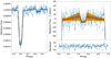 |
Fig. 14 Primary transit, secondary eclipse, and the phase variation of K2-106b with 1σ and 2σ model uncertainties (ref. Fig. 4). |
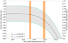 |
Fig. 15 Constraints on the geometric albedo and the dayside temperature of K2-106b (ref. Fig. 5). The maximum geometric albedo is 0.9 ± 0.3, while the maximum dayside temperature is 3620(+160/–200) K. |
5.7 K2-229 b
K2-229b orbits an active late G dwarf in a ~14 hr orbit. With a mass of 2.59 M⊕ and a radiusof 1.14 R⊕, it is believed to have a Mercury-like composition (Santerne et al. 2018). Our simultaneous analysis provides a secondary eclipse depth  ppm at more than 2σ confidence level with an amplitude of phase variation being consistent with zero
  ppm. Not much can be inferred about the nightside emission due to the poor precision on both δec and Aph. The phase-foldedlight curve, along with the best-fit model, is shown in Fig. 16.
The Ag -Td diagram in Fig. 17 indicates a maximum geometric albedo of  , while the maximum dayside temperature is
  K. These outcomes should be taken with caution, because the model selection performed in Sect. 5.9 does not favor the secondary eclipse model for K2-229b. More analyses will thus be needed to properly assess the robustness of the K2-229b occultation signal.
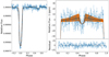 |
Fig. 16 Primary transit, secondary eclipse, and the phase variation of K2-229b with 1σ model uncertainties (ref. Fig. 4). |
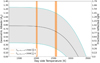 |
Fig. 17 Constraints on the geometric albedo and the dayside temperature of K2-229b (ref. Fig. 5). The geometric albedo at saturation is 0.7 ± 0.3, while the maximum dayside temperature is 3200 K. |
5.8 K2-312 b
K2-312b orbits an active F main-sequence star in a ~17 h orbit. The planet’s mass and radius is 5.6 M⊕ and 1.61 R⊕, respectively, thereby suggesting a rocky Earth-like composition with no thick atmosphere (Frustagli et al. 2020). Our analysis indicates a secondary eclipse depth of δec = 8.1 ± 3.7 ppm at a confidence level of 2.2 σ. However, we could not detect the phase curve variation as its amplitude is consistent with zero (2.7 ± 3.5 ppm). The plot of the best-fit transit, secondary eclipse, and phase curve model over the phase-folded binned data is shown in Fig. 18.
Despite the large uncertainty on δec, we estimated Ag as a function of Td. Figure 19 shows that the maximum dayside temperature is 3476 K for 100% thermal emission. On the other end, the upper limit on the geometric albedo for 100% reflection is 0.5 ± 0.2.
5.9 Summary and model selection using the Akaike Information Criterion
By using the publicly available high-precision Kepler photometry, we modeled the secondary eclipses and phase curve variations of eight ultra-short-period sub-Neptunes. We confirm previous detections of secondary eclipse for the three USP planets Kepler-10b, Kepler-78b, and K2-141b, and a marginal detection for K2-312b. We report four new discoveries of secondary eclipses for the planets Kepler-407b (3.0σ), K2-106b (3.3σ), K2-131b (3.2σ), and hints toward K2-229b (2.5σ) and K2-312b(2.2σ), however, with relatively low significance given the very shallow signals. We also detected the phase variations with confidence levels from 2 to 10σ for all planets, except K2-229b and K2-312b.
For the low-significance signals, namely, all the systems but Kepler-10, Kepler-78, and K2-141, we computed the values of the Akaike Information Criterion (AIC) for (i) the model with the secondary eclipse and phase variation, except for K2-312 and K2-229, for which we only considered the eclipse depth model, as the amplitude of their phase variation is not significant and (ii) a constant (flat) model. The ΔAIC values for Kepler-407b, K2-131b, K2-106b, and K2-312b in favor of the planetary model are equal to 6.4, 9.4, 10.0, 9.2, respectively, and would thus indicate “strong evidence” for the presence of the secondary eclipse and phase variation (Kass & Raftery 1995). None of these ΔAIC values is so high to claim “very strong evidence” (ΔAIC > 10), which is, however, expected for secondary eclipses detected at the ~ 2−3σ level. In constrast, however, the ΔAIC ~ 1 for K2-229b does not provide any “positive evidence” in favor of the secondary eclipse model. We interpret this as a warning that the detection of the secondary eclipse of K2-229b may be spurious. Further analyses, going beyond the scope of this paper, are needed to investigate the occultation signal of this planet.
The AIC model selection is just as much a Bayesian procedure as is the BIC model selection (Burnham & Anderson 2004). However, in our specific cases, the BIC may penalize complex models (e.g., phase curve and secondary eclipse models against flat out of transit models) more strongly than the AIC. This is due to the large number of data points in the light curves and the very small planetary signals with amplitudes less than the scatter of the data.
From the measured occultation depths, we estimated the geometric albedo Ag as a function of the average dayside temperature, Td, for each planet. We then provided an upper limit on both Ag and Td in the case of a purely reflective (100% reflection) or purely absorbing (100% thermal emission) planet, respectively.
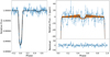 |
Fig. 18 Primary transit, secondary eclipse and the phase variation of K2-312b with 1σ model uncertainties (ref. Fig. 4). |
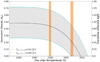 |
Fig. 19 Constraints on the geometric albedo, and the dayside temperature of K2-312b (ref. Fig. 5). The maximum geometric albedo is 0.5 ± 0.2, while the maximum dayside temperature is 3476(+228∕−305) K. |
6 Discussion and conclusion
Optical data only cannot break the degeneracy between reflected and thermally emitted light. Nevertheless, the analysis of the optical Kepler photometry in the present work leads to some important constraints. For instance, by comparing the eclipse depth, δec, and the phase variation amplitude, Aph, we unveiled nightside emission for Kepler-10b and Kepler-78b, and possibly Kepler-407b and K2-106b. Assuming that the dayside cannot be colder than the nightside, we obtained a lower limit on the dayside temperature, namely, Td ≳ Tn, which is comparable to the maximum theoretical value Td,max from thermal equilibrium considerations (see Sects. 5.1 and 5.2, along with related Figs. 5 and 7). This implies planetary temperatures hotter than Td,max, possibly due to heat retention through greenhouse effects of a high molecular weight collisional atmosphere.
The bulk density measured for the planets considered in this work indicates that they do not host a primary, hydrogen-dominated atmosphere, which was likely lost swiftly given the action of the intense stellar irradiation (e.g., Lopez 2017; Kubyshkina et al. 2018). Therefore, these planets may have quickly developed a secondary, possibly CO2-dominated, atmosphere as a result of volcanic activity or magma ocean outgassing (e.g., Elkins-Tanton 2008). Furthermore, if the secondary atmosphere formed while the star was still active, mass-loss driven by the intense stellar irradiation would have led to a complete escape also of this secondary atmosphere (e.g., Kulikov et al. 2006; Tian 2009), leaving behind a magma ocean on the dayside that would release heavy metals into an exosphere through non-thermal processes such as sputtering (e.g., Pfleger et al. 2015; Vidotto et al. 2018). However, an exosphere would not be able to redistribute heat because of its non-collisional nature and the magma ocean would be present only on the dayside, leaving a cold nightside (Léger et al. 2011).
Kepler-78b orbits a young star (Sanchis-Ojeda et al. 2013). It is therefore possible that this planet still hosts part of the CO2-dominated atmosphere released following the loss of the primary hydrogen-dominated atmosphere. Indeed, the youth of the host star and the small orbital distance pose the condition for the presence of induction heating in the planetary interior (Kislyakova et al. 2017), which would significantly strengthen surface volcanism and outgassing counteracting escape (Kislyakova et al. 2018; Kislyakova & Noack 2020). If this secondary atmosphere is dense enough to be collisional, then heat could be carried from the day to the nightside. Furthermore, Kepler-78b orbits inside the Alfvén radius of the star (Strugarek et al. 2019), thus powering magnetic star-planet interactions that may provide further energy heating up the planetary atmosphere.
In contrast, Kepler-10b orbits an old star (Fogtmann-Schulz et al. 2014) suggesting that the secondary atmosphere that was built up initially may have already been lost and that neither induction heating nor magnetic star-planet interaction would be present to support a collisional atmosphere against escape. However, a further secondary, CO2-dominated atmosphere may have built up over time from outgassing of the magma ocean present on the dayside as a result of the decreasing strength of mass loss with time due to the decreasing amount of high-energy radiation emitted by late-type stars with increasing age.
The scenario of magma-ocean planets with no heat redistribution as described by Léger et al. (2011) may apply to both K2-141b and K2-131b. Indeed, for both planets we found fully consistent values of δec and Aph, hence, there is no evidence for a significant nightside emission. For Kepler-407b, K2-106b, K2-229b, and K2-312b, the great uncertainties on δec and Aph prevent us from deriving useful constraints on possible nightside emissions.
As mentioned before, solely optical photometry does not allow us to precisely measure geometric albedos. It is still debated whether the albedos of USP small planets should be prevalently high or low. High albedos (Ag > 0.2) would require clouds of substantial reflective molecules in the secondary atmosphere (Demory 2014). Alternatively, for near-airless planets, high albedos could be the result of specular reflections from the moderately wavy lava surfaces made of metallic species such as iron oxides (Modirrousta-Galian et al. 2021). However, low albedos (Ag ≲ 0.1) have also been predicted for lava-ocean planets under a different theoretical framework by Essack et al. (2020). In this case, the occultation signal would be mostly due to high thermal emission (e.g. Figs. 11, 13). Moreover, we found that the corresponding brightness temperatures for very low albedos and no heat redistribution (Sheets & Deming 2017) might be even higher than the maximum theoretical estimates. This would imply additional heat sources such as internal tidal or magnetic heating (e.g. Lanza 2021).
Constraining the Bond albedo (AB) and the circulation efficiency (ϵ) requires a couple of assumptions, specifically: a scattering relationship between the Bond albedo and the geometric albedo, which we assumed isotropic in this work, and thermal equilibrium between the received stellar irradiation and the planet emission. Future infrared observations, for instance, with the forthcoming James Webb Space Telescope (Deming et al. 2009), should permit the degeneracy between the reflected and thermally emitted light to be broken and could also provide more precise Ag, Td, and ϵ estimates. These values, in turn, will yield valuable information on the surface or atmospheric properties of USP small planets and will greatly help in understanding the nature of these extreme worlds.
Acknowledgements
We acknowledge the computing centre of INAF – Osservatorio Astrofisico di Catania, under the coordination of the CHIPP project, for the availability of computing resources and support. We acknowledge financial contribution from the agreement ASI-INAF no. 2018-16-HH. This research has made use of the NASA Exoplanet Archive, which is operated by the California Institute of Technology, under contract with the National Aeronautics and Space Administration under the Exoplanet Exploration Program. This research has also made use of publicly available Kepler data via the MAST archive and therefore, we acknowledge the funding for the Kepler space mission provided by the NASA Science Mission Directorate and Space Telescope Science Institute (STScI) for maintaining the archive.
Appendix A Posterior distribution of the model parameters
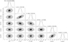 |
Fig. A.1 Posterior distribution of the best-fit model parameter of Kepler-10b. |
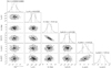 |
Fig. A.2 Posterior distribution of the best-fit model parameter of Kepler-78b. |
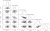 |
Fig. A.3 Posterior distribution of the best-fit model parameter of Kepler-407b. |
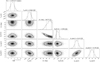 |
Fig. A.4 Posterior distribution of the best-fit model parameter of K2-141b. |
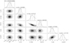 |
Fig. A.5 Posterior distribution of the best-fit model parameter of K2-131b. |
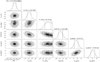 |
Fig. A.6 Posterior distribution of the best-fit model parameter of K2-106b. |
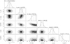 |
Fig. A.7 Posterior distribution of the best-fit model parameter of K2-229b. |
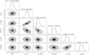 |
Fig. A.8 Posterior distribution of the best-fit model parameter of K2-312b. |
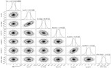 |
Fig. A.9 Posterior distribution of the best-fit model parameter of Kepler-10b including phase offset as a free parameter. Posteriors for the phase offset is consistent with zero. |
Appendix B Detrending of stellar variability using Gaussian processes
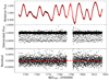 |
Fig. B.1 Light curve detrending using Gaussian processes. Top: K2-141 light curve after removing the transits of planet c and with the GP model in red. Middle: Light curve minus the GP model. Bottom: residual of the combined GP + transit, eclipse and the phase variation best-fit model. |
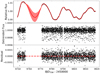 |
Fig. B.2 Light curve detrending of K2-229 using Gaussian processes after removing the transits of K2-229c and K2-229d (ref. Fig. B.1) |
References
- Adams, E. R., Jackson, B., Endl, M., et al. 2017, AJ, 153, 82 [NASA ADS] [CrossRef] [Google Scholar]
- Barragán, O., Gandolfi, D., Dai, F., et al. 2018, A&A, 612, A95 [Google Scholar]
- Batalha, N. M., Borucki, W. J., Bryson, S. T., et al. 2011, ApJ, 729, 27 [Google Scholar]
- Bertocco, S., Goz, D., Tornatore, L., et al. 2020, in ASP Conf. Ser., 527, Astronomical Data Analysis Software and Systems XXIX, eds. R. Pizzo, E. R. Deul, J. D. Mol, J. de Plaa, & H. Verkouter, 303 [NASA ADS] [Google Scholar]
- Bonomo, A. S., Chabaud, P. Y., Deleuil, M., et al. 2012, A&A, 547, A110 [NASA ADS] [CrossRef] [EDP Sciences] [Google Scholar]
- Brown, T. M., Latham, D. W., Everett, M. E., & Esquerdo, G. A. 2011, AJ, 142, 112 [Google Scholar]
- Burnham, K. P., & Anderson, D. R. 2004, Sociol. Methods Res., 33, 261 [Google Scholar]
- Carrera, D., Ford, E. B., Izidoro, A., et al. 2018, ApJ, 866, 104 [Google Scholar]
- Castelli, F., & Kurucz, R. L. 2003, in IAU Symp., 210, Modelling of Stellar Atmospheres, eds. N. Piskunov, W. W. Weiss, & D. F. Gray, A20 [Google Scholar]
- Choi, J., Dotter, A., Conroy, C., et al. 2016, ApJ, 823, 102 [Google Scholar]
- Cowan, N. B., & Agol, E. 2011, ApJ, 729, 54 [Google Scholar]
- Cutri, R. M., et al. 2014, VizieR Online Data Catalog: II/328 [Google Scholar]
- Dai, F., Winn, J. N., Gandolfi, D., et al. 2017, AJ, 154, 226 [CrossRef] [Google Scholar]
- Dai, F., Masuda, K., Winn, J. N., & Zeng, L. 2019, ApJ, 883, 79 [NASA ADS] [CrossRef] [Google Scholar]
- Dawson, R. I., & Fabrycky, D. C. 2010, ApJ, 722, 937 [Google Scholar]
- Deming, D., Seager, S., Winn, J., et al. 2009, PASP, 121, 952 [NASA ADS] [CrossRef] [Google Scholar]
- Demory, B.-O. 2014, ApJ, 789, L20 [NASA ADS] [CrossRef] [Google Scholar]
- Demory, B. O., Gillon, M., Deming, D., et al. 2011, A&A, 533, A114 [NASA ADS] [CrossRef] [EDP Sciences] [Google Scholar]
- Demory, B.-O., Gillon, M., de Wit, J., et al. 2016a, Nature, 532, 207 [NASA ADS] [CrossRef] [Google Scholar]
- Demory, B.-O., Gillon, M., Madhusudhan, N., & Queloz, D. 2016b, MNRAS, 455, 2018 [NASA ADS] [CrossRef] [Google Scholar]
- Dotter, A. 2016, ApJS, 222, 8 [Google Scholar]
- Dumusque, X., Bonomo, A. S., Haywood, R. D., et al. 2014, ApJ, 789, 154 [NASA ADS] [CrossRef] [Google Scholar]
- Eastman, J., Gaudi, B. S., & Agol, E. 2013, PASP, 125, 83 [Google Scholar]
- Eastman, J. D., Rodriguez, J. E., Agol, E., et al. 2019, PASP submitted [arXiv:1907.09480] [Google Scholar]
- Elkins-Tanton, L. T. 2008, Earth Planet. Sci. Lett., 271, 181 [Google Scholar]
- Essack, Z., Seager, S., & Pajusalu, M. 2020, ApJ, 898, 160 [CrossRef] [Google Scholar]
- Esteves, L. J., De Mooij, E. J. W., & Jayawardhana, R. 2013, ApJ, 772, 51 [NASA ADS] [CrossRef] [Google Scholar]
- Esteves, L. J., De Mooij, E. J. W., & Jayawardhana, R. 2015, ApJ, 804, 150 [Google Scholar]
- Fogtmann-Schulz, A., Hinrup, B., Van Eylen, V., et al. 2014, ApJ, 781, 67 [NASA ADS] [CrossRef] [Google Scholar]
- Foreman-Mackey, D. 2018, Res. Notes Am. Astron. Soc., 2, 31 [NASA ADS] [Google Scholar]
- Foreman-Mackey, D., Hogg, D. W., Lang, D., & Goodman, J. 2013, PASP, 125, 306 [Google Scholar]
- Foreman-Mackey, D., Agol, E., Ambikasaran, S., & Angus, R. 2017, AJ, 154, 220 [Google Scholar]
- Fressin, F., Torres, G., Désert, J.-M., et al. 2011, ApJS, 197, 5 [NASA ADS] [CrossRef] [Google Scholar]
- Frustagli, G., Poretti, E., Milbourne, T., et al. 2020, A&A, 633, A133 [NASA ADS] [CrossRef] [EDP Sciences] [Google Scholar]
- Gaia Collaboration (Brown, A. G. A., et al.) 2018, A&A, 616, A1 [NASA ADS] [CrossRef] [EDP Sciences] [Google Scholar]
- Giménez, A. 2006, A&A, 450, 1231 [NASA ADS] [CrossRef] [EDP Sciences] [Google Scholar]
- Greiss, S., Steeghs, D., Gänsicke, B. T., et al. 2012, AJ, 144, 24 [NASA ADS] [CrossRef] [Google Scholar]
- Guenther, E. W., Barragán, O., Dai, F., et al. 2017, A&A, 608, A93 [NASA ADS] [CrossRef] [EDP Sciences] [Google Scholar]
- Haywood, R. D., Collier Cameron, A., Queloz, D., et al. 2014, MNRAS, 443, 2517 [Google Scholar]
- Henden, A. A., Levine, S., Terrell, D., & Welch, D. L. 2015, in American Astronomical Society Meeting Abstracts, 225, 336.16 [NASA ADS] [Google Scholar]
- Howard, A. W., Sanchis-Ojeda, R., Marcy, G. W., et al. 2013, Nature, 503, 381 [CrossRef] [Google Scholar]
- Hu, R., Demory, B.-O., Seager, S., Lewis, N., & Showman, A. P. 2015, ApJ, 802, 51 [Google Scholar]
- Isella, A., Testi, L., & Natta, A. 2006, A&A, 451, 951 [NASA ADS] [CrossRef] [EDP Sciences] [Google Scholar]
- Ito, Y., Ikoma, M., Kawahara, H., et al. 2015, ApJ, 801, 144 [NASA ADS] [CrossRef] [Google Scholar]
- Jansen, T., & Kipping, D. 2018, MNRAS, 478, 3025 [NASA ADS] [CrossRef] [Google Scholar]
- Kass, R. E., & Raftery, A. E. 1995, J. Am. Stat. Assoc., 90, 773 [Google Scholar]
- Kipping, D. M. 2010, MNRAS, 408, 1758 [Google Scholar]
- Kislyakova, K., & Noack, L. 2020, A&A, 636, L10 [NASA ADS] [CrossRef] [EDP Sciences] [Google Scholar]
- Kislyakova, K. G., Noack, L., Johnstone, C. P., et al. 2017, Nat. Astron., 1, 878 [NASA ADS] [CrossRef] [Google Scholar]
- Kislyakova, K. G., Fossati, L., Johnstone, C. P., et al. 2018, ApJ, 858, 105 [NASA ADS] [CrossRef] [Google Scholar]
- Kubyshkina, D., Fossati, L., Erkaev, N. V., et al. 2018, A&A, 619, A151 [NASA ADS] [CrossRef] [EDP Sciences] [Google Scholar]
- Kulikov, Y. N., Lammer, H., Lichtenegger, H. I. M., et al. 2006, Planet. Space Sci., 54, 1425 [NASA ADS] [CrossRef] [Google Scholar]
- Lanza, A. F. 2021, A&A, 653, A112 [NASA ADS] [CrossRef] [EDP Sciences] [Google Scholar]
- Lecavelier Des Etangs, A. 2007, A&A, 461, 1185 [NASA ADS] [CrossRef] [EDP Sciences] [Google Scholar]
- Léger, A., Grasset, O., Fegley, B., et al. 2011, Icarus, 213, 1 [CrossRef] [Google Scholar]
- Lopez, E. D. 2017, MNRAS, 472, 245 [NASA ADS] [CrossRef] [Google Scholar]
- Lopez, E., & Fortney, J. J. 2013, in AAS/Division for Planetary Sciences Meeting Abstracts #45, 200.08 [Google Scholar]
- López-Morales, M., & Seager, S. 2007, ApJ, 667, L191 [CrossRef] [Google Scholar]
- Malavolta, L., Mayo, A. W., Louden, T., et al. 2018, AJ, 155, 107 [NASA ADS] [CrossRef] [Google Scholar]
- Mandel, K., & Agol, E. 2002, ApJ, 580, L171 [Google Scholar]
- Marcy, G. W., Isaacson, H., Howard, A. W., et al. 2014, ApJS, 210, 20 [NASA ADS] [CrossRef] [Google Scholar]
- Miguel, Y., Kaltenegger, L., Fegley, B., & Schaefer, L. 2011, ApJ, 742, L19 [NASA ADS] [CrossRef] [Google Scholar]
- Modirrousta-Galian, D., Ito, Y., & Micela, G. 2021, Icarus, 358, 114175 [CrossRef] [Google Scholar]
- Nelson, B. E., Ford, E. B., Wright, J. T., et al. 2014, MNRAS, 441, 442 [Google Scholar]
- Owen, J. E., & Wu, Y. 2017, ApJ, 847, 29 [Google Scholar]
- Pepe, F., Cameron, A. C., Latham, D. W., et al. 2013, Nature, 503, 377 [NASA ADS] [CrossRef] [Google Scholar]
- Perryman, M. 2011, The Exoplanet Handbook (Cambridge University Press, 2011), 103 [CrossRef] [Google Scholar]
- Pfleger, M., Lichtenegger, H. I. M., Wurz, P., et al. 2015, Planet. Space Sci., 115, 90 [CrossRef] [Google Scholar]
- Pont, F., Zucker, S., & Queloz, D. 2006, MNRAS, 373, 231 [NASA ADS] [CrossRef] [Google Scholar]
- Rowe, J. F., Matthews, J. M., Seager, S., et al. 2006, ApJ, 646, 1241 [NASA ADS] [CrossRef] [Google Scholar]
- Sanchis-Ojeda, R., Rappaport, S., Winn, J. N., et al. 2013, ApJ, 774, 54 [Google Scholar]
- Sanchis-Ojeda, R., Rappaport, S., Winn, J. N., et al. 2014, ApJ, 787, 47 [Google Scholar]
- Santerne, A., Brugger, B., Armstrong, D. J., et al. 2018, Nat. Astron., 2, 393 [Google Scholar]
- Schaefer, L., & Fegley, B. 2004, Icarus, 169, 216 [CrossRef] [Google Scholar]
- Schaefer, L., & Fegley, B. 2009, ApJ, 703, L113 [CrossRef] [Google Scholar]
- Schaefer, L., Lodders, K., & Fegley, B. 2012, ApJ, 755, 41 [NASA ADS] [CrossRef] [Google Scholar]
- Sheets, H. A., & Deming, D. 2014, ApJ, 794, 133 [NASA ADS] [CrossRef] [Google Scholar]
- Sheets, H. A., & Deming, D. 2017, AJ, 154, 160 [CrossRef] [Google Scholar]
- Sing, D. K. 2010, A&A, 510, A21 [NASA ADS] [CrossRef] [EDP Sciences] [Google Scholar]
- Sinukoff, E., Howard, A. W., Petigura, E. A., et al. 2017, AJ, 153, 271 [CrossRef] [Google Scholar]
- Snellen, I. A. G., de Mooij, E. J. W., & Albrecht, S. 2009, Nature, 459, 543 [NASA ADS] [CrossRef] [Google Scholar]
- Stassun, K. G., & Torres, G. 2018, ApJ, 862, 61 [Google Scholar]
- Strugarek, A., Brun, A. S., Donati, J. F., Moutou, C., & Réville, V. 2019, ApJ, 881, 136 [Google Scholar]
- Taffoni, G., Becciani, U., Garilli, B., et al. 2020, in ASP Conf. Ser., 527, Astronomical Data Analysis Software and Systems XXIX, eds. R. Pizzo, E. R. Deul, J. D. Mol, J. de Plaa, & H. Verkouter, 307 [NASA ADS] [Google Scholar]
- Ter Braak, C. J. F. 2006, Stat. Comput., 16, 239 [Google Scholar]
- Tian, F. 2009, ApJ, 703, 905 [NASA ADS] [CrossRef] [Google Scholar]
- Vanderburg, A., & Johnson, J. A. 2014, PASP, 126, 948 [Google Scholar]
- Vanderburg, A., Latham, D. W., Buchhave, L. A., et al. 2016, ApJS, 222, 14 [Google Scholar]
- Vanderburg, A., Becker, J. C., Buchhave, L. A., et al. 2017, AJ, 154, 237 [NASA ADS] [CrossRef] [Google Scholar]
- Vidotto, A. A., Lichtenegger, H., Fossati, L., et al. 2018, MNRAS, 481, 5296 [Google Scholar]
- Weiss, L. M., Rogers, L. A., Isaacson, H. T., et al. 2016, ApJ, 819, 83 [NASA ADS] [CrossRef] [Google Scholar]
- Weiss, L. M., Deck, K. M., Sinukoff, E., et al. 2017, AJ, 153, 265 [NASA ADS] [CrossRef] [Google Scholar]
- Winn, J. N. 2010, Exoplanet Transits and Occultations, ed. S. Seager, 55 [Google Scholar]
- Winn, J. N., Matthews, J. M., Dawson, R. I., et al. 2011, ApJ, 737, L18 [Google Scholar]
- Winn, J. N., Sanchis-Ojeda, R., Rogers, L., et al. 2017, AJ, 154, 60 [NASA ADS] [CrossRef] [Google Scholar]
- Winn, J. N., Sanchis-Ojeda, R., & Rappaport, S. 2018, New Astron. Rev., 83, 37 [CrossRef] [Google Scholar]
- Zacharias, N., Finch, C. T., Girard, T. M., et al. 2012, VizieR Online Data Catalog: I/322A [Google Scholar]
The INAF hotcat cluster (Taffoni et al. 2020; Bertocco et al. 2020) was used for the analyses.
δnight is missing the tiny fraction of the nightside flux which is facing away from the observer while Aph(ϕt1, ϕt4) includes that same tiny fraction of the nightside flux, this time facing towards the observer.
All Tables
Stellar parameters from the SED fitting and the MIST evolutionary tracks (Eastman et al. 2019).
Comparison of the transit, secondary eclipse and the phase curve model parameters of K2-141b with two different detrending techniques, namely the sliding linear fitting and Gaussian processes.
Best-fit parameters and associated uncertainties from our fit of primary transits, secondary eclipses, and phase variations.
All Figures
|
Fig. 1 Detrending of the stellar variability in the light curve of K2-141 using the sliding linear fitting. Top: K2-141 light curve after removing the transits of planet c; the SLF model is over-plotted in red. Middle: detrended light curve. Bottom: residual of the model with the best-fit planetary parameters. |
| In the text | |
|
Fig. 2 Gaussian-process detrending of the stellar variability in the light curve of K2-131. Top: light curve with the GP model over-plotted in red. Middle: detrended light curve. Bottom: best-fit residuals of the combined fit. The GP detrending and model fitting are carried out simultaneously, unlike the SLF detrending. |
| In the text | |
|
Fig. 3 Phase curve of a circular orbit around the secondary eclipse showing the difference flux reference levels. The duration of the secondary eclipse is equal to the transit duration. The times t1, t2, t3, and t4 define the ingress and egress moments of the planetary occultation in the same way as T1, T2, T3, T4 for the primary transit. The eclipse depth is actually the difference between the flux references of planet’s brightness at t1 ∕t4 and the stellar brightness at t2∕t3. |
| In the text | |
|
Fig. 4 Planetary light curve showing the primary transit, secondary eclipse and the phase variation. Left: detrended, phase-folded, and binned light curve of Kepler-10b (blue points). The best-fit model is over-plotted in solid black line. Right: enlarged view of the secondary eclipse and phase variation. Uncertainties of the best-fit model are shown at 1σ and 3σ in dark and light orange, respectively. The residuals of the best-fit model are displayed in the bottom. |
| In the text | |
|
Fig. 5 Geometric albedo (Ag) estimated as a function of the dayside temperature of Kepler-10b. The cyan lines correspond to the 3σ uncertainty in the computation of Ag. The two vertical red lines and orange regions display the theoretical temperatures and associated 1σ error bars, by considering zero Bond albedo and negligible or perfect heat redistribution. The maximum geometric albedo is at 0.74 ± 0.06. The maximum dayside temperature can be as high as 3430(+50∕−40) K in the case of100% thermal emission. |
| In the text | |
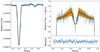 |
Fig. 6 Primary transit, secondary eclipse, and the phase variation of Kepler-78b (ref. Fig. 4). |
| In the text | |
|
Fig. 7 Constraints on the geometric albedo and the dayside temperature of Kepler-78b (ref. Fig. 5). The maximum geometric albedo is 0.48 ± 0.06. The maximum dayside temperature is 3060(+40∕−50) K in the case of100% thermal emission. |
| In the text | |
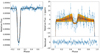 |
Fig. 8 Primary transit, secondary eclipse, and the phase variation of Kepler-407b (ref. Fig. 4). |
| In the text | |
|
Fig. 9 Constraints on the geometric albedo and the dayside temperature of Kepler-407b (ref. Fig. 5). The geometric albedo at saturation is 0.56(+0.19∕−0.18), while the maximum dayside temperature is 3270 ± 140 K. |
| In the text | |
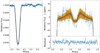 |
Fig. 10 Primary transit, secondary eclipse, and the phase variation of K2-141b (ref. Fig. 4). |
| In the text | |
|
Fig. 11 Constraints on the geometric albedo and the dayside temperature of K2-141b (ref. Fig. 5). The maximum geometric albedo is 0.34 ± 0.05, while the maximum dayside temperature is 2860(+50∕−60) K. |
| In the text | |
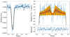 |
Fig. 12 Primary transit, secondary eclipse, and the phase variation of K2-131b (ref. Fig. 4). |
| In the text | |
|
Fig. 13 Constraints on the geometric albedo and the dayside temperature of K2-131b (ref. Fig. 5). The maximum geometric albedo is 0.55(+0.18∕−0.17), while the maximum dayside temperature is 3320(+140∕−180) K. |
| In the text | |
|
Fig. 14 Primary transit, secondary eclipse, and the phase variation of K2-106b with 1σ and 2σ model uncertainties (ref. Fig. 4). |
| In the text | |
|
Fig. 15 Constraints on the geometric albedo and the dayside temperature of K2-106b (ref. Fig. 5). The maximum geometric albedo is 0.9 ± 0.3, while the maximum dayside temperature is 3620(+160/–200) K. |
| In the text | |
|
Fig. 16 Primary transit, secondary eclipse, and the phase variation of K2-229b with 1σ model uncertainties (ref. Fig. 4). |
| In the text | |
|
Fig. 17 Constraints on the geometric albedo and the dayside temperature of K2-229b (ref. Fig. 5). The geometric albedo at saturation is 0.7 ± 0.3, while the maximum dayside temperature is 3200 K. |
| In the text | |
|
Fig. 18 Primary transit, secondary eclipse and the phase variation of K2-312b with 1σ model uncertainties (ref. Fig. 4). |
| In the text | |
|
Fig. 19 Constraints on the geometric albedo, and the dayside temperature of K2-312b (ref. Fig. 5). The maximum geometric albedo is 0.5 ± 0.2, while the maximum dayside temperature is 3476(+228∕−305) K. |
| In the text | |
|
Fig. A.1 Posterior distribution of the best-fit model parameter of Kepler-10b. |
| In the text | |
|
Fig. A.2 Posterior distribution of the best-fit model parameter of Kepler-78b. |
| In the text | |
|
Fig. A.3 Posterior distribution of the best-fit model parameter of Kepler-407b. |
| In the text | |
|
Fig. A.4 Posterior distribution of the best-fit model parameter of K2-141b. |
| In the text | |
|
Fig. A.5 Posterior distribution of the best-fit model parameter of K2-131b. |
| In the text | |
|
Fig. A.6 Posterior distribution of the best-fit model parameter of K2-106b. |
| In the text | |
|
Fig. A.7 Posterior distribution of the best-fit model parameter of K2-229b. |
| In the text | |
|
Fig. A.8 Posterior distribution of the best-fit model parameter of K2-312b. |
| In the text | |
|
Fig. A.9 Posterior distribution of the best-fit model parameter of Kepler-10b including phase offset as a free parameter. Posteriors for the phase offset is consistent with zero. |
| In the text | |
|
Fig. B.1 Light curve detrending using Gaussian processes. Top: K2-141 light curve after removing the transits of planet c and with the GP model in red. Middle: Light curve minus the GP model. Bottom: residual of the combined GP + transit, eclipse and the phase variation best-fit model. |
| In the text | |
|
Fig. B.2 Light curve detrending of K2-229 using Gaussian processes after removing the transits of K2-229c and K2-229d (ref. Fig. B.1) |
| In the text | |
Current usage metrics show cumulative count of Article Views (full-text article views including HTML views, PDF and ePub downloads, according to the available data) and Abstracts Views on Vision4Press platform.
Data correspond to usage on the plateform after 2015. The current usage metrics is available 48-96 hours after online publication and is updated daily on week days.
Initial download of the metrics may take a while.