| Issue |
A&A
Volume 657, January 2022
|
|
|---|---|---|
| Article Number | L11 | |
| Number of page(s) | 9 | |
| Section | Letters to the Editor | |
| DOI | https://doi.org/10.1051/0004-6361/202142789 | |
| Published online | 12 January 2022 | |
Letter to the Editor
Abundance of beryllium in the Sun and stars: The role of non-local thermodynamic equilibrium effects
1
Crimean Astrophysical Observatory, Nauchny 298409, Crimea
e-mail: This email address is being protected from spambots. You need JavaScript enabled to view it.
2
Institute of Theoretical Physics and Astronomy, Vilnius University, Saulėtekio Al. 3, Vilnius 10257, Lithuania
Received:
30
November
2021
Accepted:
28
December
2021
Abstract
Context. Earlier studies have suggested that deviations from the local thermodynamic equilibrium (LTE) play a minor role in the formation of Be II 313 nm resonance lines in solar and stellar atmospheres. Recent improvements in the atomic data allow a more complete model atom of Be to be constructed and the validity of these claims to be reassessed using more up-to-date atomic physics.
Aims. The main goal of this study therefore is to refocus on the role of non-local thermodynamic equilibrium (NLTE) effects in the formation of Be II 313.04 and 313.11 nm resonance lines in solar and stellar atmospheres.
Methods. For this, we constructed a model atom of Be using new atomic data that recently became available. The model atom contains 98 levels and 383 radiative transitions of Be I and Be II and uses the most up-to-date collision rates with electrons and hydrogen. This makes it the most complete model atom used to determine 1D NLTE solar Be abundance and to study the role of NLTE effects in the formation of Be II 313 nm resonance lines.
Results. We find that deviations from LTE have a significant influence on the strength of the Be II 313 nm line in solar and stellar atmospheres. For the Sun, we obtained the 1D NLTE Be abundance of A(Be)NLTE = 1.32 ± 0.05, which is in excellent agreement with the meteoritic value of A(Be) = 1.31 ± 0.04. Importantly, we find that NLTE effects become significant in FGK stars. Moreover, there is a pronounced variation in 1D NLTE–LTE abundance corrections with the effective temperature and metallicity. Therefore, contrary to our previous understanding, the obtained results indicate that NLTE effects play an important role in Be line formation in stellar atmospheres and have to be properly taken into account in Be abundance studies, especially in metal-poor stars.
Key words: Sun: abundances / stars: abundances / stars: late-type / techniques: spectroscopic / line: formation
© ESO 2022
1. Introduction
Studies of Be abundance are of interest in various astrophysical contexts. Because Be is synthesised mostly via the cosmic ray spallation in the interstellar medium (e.g. Smiljanic et al. 2021) and is quickly destroyed in stars (but see Tucci Maia et al. 2015), Be may serve as a useful tracer of mixing in stellar interiors (e.g. Smiljanic et al. 2010). In the context of Galactic chemical evolution, Be may provide valuable information about the composition and role of cosmic rays in the chemical enrichment of Galactic interstellar matter (e.g. Prantzos 2012).
The only Be abundance indicators in the optical range are Be II resonance lines located at 313.04 and 313.11 nm. Earlier studies have shown that non-local thermodynamic equilibrium (NLTE) effects lead to strong over-ionisation of Be I in the solar atmosphere, with a significant increase in Be II concentration in the Be II 313 nm line-forming region (Asplund 2005). This is because the strongest lines and the ionisation cutoff of Be II are located in the UV, where solar radiative flux exceeds that of the Planck function; this leads to the over-ionisation of Be I. For the same reason, the higher levels of Be II become overpopulated and the lowest levels underpopulated. Thus, the first effect makes Be II lines appear stronger and the second weaker. A number of studies performed until now have suggested that the two processes effectively cancel each other out and lead to a zero NLTE–LTE (local thermodynamic equilibrium) Be abundance correction for the Sun (Garcia Lopez et al. 1995; Takeda et al. 2011). With this, the ‘standard’ solar photospheric Be abundance, A(Be) = 1.38 ± 0.09 (Asplund et al. 2021), is slightly higher than that measured in meteorites, A(Be) = 1.31 ± 0.04 (Lodders 2021).
Amongst the most important advances in Be abundance studies, new atomic data recently became available. In this context, collisional cross-sections with electrons and hydrogen obtained from quantum mechanical computations by Dipti (2019) and Yakovleva et al. (2016) are of particular interest as these effects play a crucial role in NLTE line formation. These atomic data were not yet available to earlier studies of Be NLTE line formation in solar and stellar atmospheres, and thus collisions were treated in a simplified fashion. Therefore, the availability of new atomic data on the one hand and the discrepancy between the photospheric and meteoritic solar Be abundances on the other made it desirable to re-determine solar Be abundance and to reassess the role of NLTE effects in Be spectral line formation, both in the Sun and other types of stars.
The motivation behind the present study was therefore threefold. First, using the most-up-to-date atomic data we constructed a new model atom of Be to assess the role of NLTE effects on the Be II 313 nm line formation in solar and stellar atmospheres. Second, the new model atom was used to obtain an updated value of 1D NLTE solar Be abundance. And finally, we investigated the role of NLTE effects on Be line formation in stellar atmospheres with a goal of providing a grid of 1D NLTE–LTE Be abundance corrections that could be used for Be abundance studies in different types of stars.
2. Methodology of 1D NLTE Be abundance analysis
2.1. Observational data
The only Be lines available for stellar abundance analysis in the optical range are those of Be II located at 313 nm. For the calibration of solar flux in this spectral range (Sect. 3.1) we a used solar irradiance spectrum obtained with the SOLar SPECtrometer (SOLSPEC) instrument of the SOLAR payload on board the International Space Station (Meftah et al. 2018). The SOLSPEC spectrum covers a range of ≈165 − 3000 nm with a resolution of ≈0.1 − 0.2 nm in the UV.
For the calibration of the solar flux in the UV–blue spectral range we also used two additional low-resolution solar irradiance flux spectra: (a) the Upper Atmosphere Research Satellite (UARS) irradiance spectrum obtained in the range of 115.0 − 420.0 nm with a resolution of ≈1 nm (Woods et al. 1996); and (b) the Compact Spectral Irradiance Monitor (CSIM) irradiance spectrum in the range of 200.0 − 2600.0 nm at ≈2 nm resolution1.
The solar flux atlas from Kurucz et al. (1984) was used for solar Be abundance determination (Sect. 3.3). It covers a range of 296 − 1300 nm and has a resolution of ≈350 000 in the near UV.
2.2. Model atom of Be
Having the first ionisation potential of 9.32 eV, Be in the atmospheres of FGK stars is available in the neutral and single-ionised states; thus, both stages should be taken into account for computing NLTE level departure coefficients. Our Be model atom therefore consists of 48 levels of Be I (n ≤ 8, l ≤ 4), 49 levels of Be II (n ≤ 12, l ≤ 5), and a ground level of Be III. Level energies were taken from the NIST database, Kramida et al. (2012), and level fine structure was not taken into account. The lowest ionisation energy for Be I (from level 8d 3D) of 0.22 eV ensures a reliable connection between the Be I and Be II stages of the model atom at T ≳ 2000 K. Ionisation energy from the highest level in the model atom of Be II is slightly higher, 0.38 eV (T ≳ 4000 K), but this is not critical, because the fraction of Be III in the atmospheres of cool stars is very small.
For the computation of departure coefficients, 230 bound–bound radiative transitions were taken into account for Be I and 153 for Be II. We used oscillator strengths from the TOPBase (Cunto et al. 1993). Importantly, the majority of Be lines are very weak, and thus uncertainties in the oscillator strengths play a negligible role. For the strongest transitions that occur from the lowest two levels of Be I, oscillator strengths were taken from Tachiev & Froese Fischer (1999), while for Be II 313 nm resonance lines we used quantum mechanical computation data from Yan et al. (1998). Photoionisation cross-sections were taken from the TOPBase for all Be I and Be II levels except for levels f and g of Be II, in which case a hydrogen-like approximation was used. Our tests have shown that one order variation in the cross-sections of levels f and g of Be II had a negligible effect on the population numbers of the lowest Be II levels.
Collision rates for the transitions between the 19 lowest levels of Be I were taken from Dipti (2019) and those for transitions between the 10 higher-lying levels (up to and including 6s 1S) from the ADAS database (Summers & O’Mullane 2011). The ADAS collisional rates were also used to account for the transitions between the 14 lowest levels of Be II. For the rest of the bound-bound collisional transitions, we adopted the formulae from van Regemorter (1962) for permitted transitions and those from Allen (1973) for the forbidden ones. Collisional ionisation rates were calculated using the formula from Seaton (1962).
To account for inelastic transitions with hydrogen, we used quantum mechanical data from Yakovleva et al. (2016) for the first 14 levels of Be I. For the remaining levels, Drawin’s approximation (Drawin 1968) was used in the form provided by Steenbock & Holweger (1984), with SH = 0.1. Variation in SH values from 0 to 1 had no effect on the line strength in the spectra of dwarf and giant stars with 3500 < Teff < 6500 K, with changes in the line equivalent width of < 0.1%. Once again, transitions from the lowest levels of Be I play a major role, and for these cases quantum mechanical data were used.
2.3. Spectral line synthesis
The ATLAS9 model atmospheres that were used in spectral line synthesis calculations were computed using opacity distribution functions (ODFs) from Mészáros et al. (2012). The ODFs were constructed using updated absorption lists of molecular lines, which is of critical importance for calculating the atmospheres of cool stars. For the calculation of synthetic spectra in the vicinity of Be II lines, level departure coefficients were computed using the MULTI code (Carlsson 1986) in the form modified by Korotin et al. (1999) to enable the use of ATLAS9 opacities. Kurucz’s ODFs (Mészáros et al. 2012) were used to account for line blanketing only when computing photoionisation rates. Synthetic spectra were produced using the SynthV code (Tsymbal et al. 2019), with Be II line profiles computed in NLTE (using the departure coefficients obtained with MULTI) and those of other lines calculated in LTE. The atomic line data were taken from the VALD3 database (Ryabchikova et al. 2015). We used data from Barklem et al. (2000) to account for the van der Waals broadening of Be II lines. For the Sun, we also used the TURBOSPECTRUM code Plez (2012) (v.19; Sects. 3.1 and 3.3).
3. NLTE effects in Be spectral line formation and Be abundances in the Sun and stars
3.1. Missing near-UV opacity in the solar spectrum
Determination of the continuum in the vicinity of Be II 313 nm resonance lines is complicated in stars of higher metallicity because this spectral range is heavily blended with various atomic and molecular lines. Inevitably, this takes a toll on the accuracy of determined Be abundances.
In addition, the accuracy of Be abundances is greatly influenced by the reliability of the continuous opacity that is used in spectral synthesis calculations. For example, Balachandran & Bell (1998) concluded that it was necessary to increase the continuum opacity by 1.6 times in the synthetic spectrum around 313 nm to obtain a reasonable fit with the observed solar flux. Fontenla et al. (2015) showed that taking absorption from the dissociation of CH, NH, and OH into account may also affect the continuous opacity noticeably. However, Carlberg et al. (2018, hereafter C18) demonstrated that even for cool stars the additional contribution from molecules does not exceed 4%. Therefore, in order to reconcile the synthetic spectrum of the Sun with the observed spectrum, an additional factor of 1.2 was introduced in C18 to increase the total opacity in the continuum. Bell et al. (2001) have concluded that an adequate description of the UV flux is obtained if the opacity due to b–f transitions of Fe I is added and increased by a factor of two. This conclusion was supported by Asplund (2004), who showed that a 50% increase in the opacity was needed to obtain O abundances from OH lines near 313 nm that are consistent with those determined using OH lines in the infrared.
To check the effects of missing opacity in our spectral synthesis calculations, we computed solar flux in the range of 250 − 400 nm with a step of 0.005 nm using the SynthV and TURBOSPECTRUM spectral synthesis packages. Both codes used identical Fe b–f opacities taken from the TOPBase (Cunto et al. 1993), and synthesis of all spectral lines was performed under the assumption of LTE. In addition, a block of opacities resulting from the dissociation of CH and NH molecules was added to the calculations, as proposed in C18. For comparison, we used the SOLSPEC, CSIM, and UARS solar irradiance spectra (Sect. 2.1) converted to flux on the solar surface. Spectral synthesis was performed using the solar ATLAS9 model computed by Castelli & Kurucz (2003)2, with the line data taken from the VALD3 database (Ryabchikova et al. 2015), solar chemical composition from Asplund et al. (2021), and a microturbulence velocity of 1 km s−1. For the comparison with observations, the resolution of the synthetic flux was degraded to that of the observed spectra.
The results of our computations demonstrate that the solar flux in the vicinity of Be lines predicted by spectral synthesis with the SynthV and TURBOSPECTRUM packages is nearly identical and, at the same time, is 25 − 30% higher than observed (Fig. 1). On the other hand, there is an excellent agreement between the observed and synthetic spectra at ≳390 nm, where the differences do not exceed 1 − 2%.
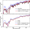 |
Fig. 1. Synthetic and observed solar fluxes in the blue–UV spectral range. Top: comparison of synthetic fluxes with the observed SOLSPEC flux. Bottom: comparison of synthetic and observed CSIM and UARS fluxes. |
To bring synthetic and observed fluxes of the Sun into agreement in the UV region, we artificially increased the b–f opacities of Fe by a factor of 2.7 at > 265.0 nm. Such an approach was adopted earlier by Bell et al. (2001), in which case the Fe opacities were increased by a factor of two. With this adjustment, we obtained a very good agreement between the synthetic fluxes computed with the SynthV and TURBOSPECTRUM codes and the observed SOLSPEC flux (Fig. 1, top panel). The adjusted synthetic spectra also agree reasonably well with the observed low-resolution CSIM and UARS fluxes (Fig. 1, bottom panel).
3.2. Modifications to the VALD3 line list
As indicated in Sect. 2.3, we used atomic line data from the VALD3 database (Ryabchikova et al. 2015) to determine the solar Be abundance. We made several further improvements related to (a) the lines that directly affect the Be abundance determination; and (b) the lines that do not affect Be abundances but give a better fit in the immediate neighbourhood of Be II lines. For this we roughly followed the prescription used by Takeda et al. (2011), Delgado Mena et al. (2012), and C18 in their solar Be abundance studies. For group (a) lines, we added the CH 313.0367 nm line from Delgado Mena et al. (2012); increased the log gf from −2.222 to −1.561 for the Ti I 313.0377 line, as suggested by Takeda et al. (2011) and Delgado Mena et al. (2012); and shifted the wavelength of the Mn I 313.1036 nm line by −0.002 nm and increased its log gf to −0.550, following the recommendation of Ashwell et al. (2005). We also made adjustments to several group (b) lines: removed the Fe I 312.9619 nm line, as recommended by C18; increased the log gf from −0.401 to −0.201 for the Cr I 313.1216 nm line; and added CH 313.0644 nm and OH 313.1366 nm lines from the list of Delgado Mena et al. (2012). We did not add any ‘hypothetical’ lines, such as the Ti II 313.1039 nm line introduced by C18 or the Fe I 313.1043 nm line by Takeda et al. (2011). The modified line list is provided in Appendix A.
The adjustments to the line list described above and the modification of the continuum opacity (Sect. 3.1) allowed us to obtain an adequate fit of the solar spectrum in the vicinity of the Be II lines (Fig. 2).
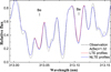 |
Fig. 2. Observed solar spectrum from the Kurucz atlas (dots) and the best-fitted synthetic SynthV spectra (solid lines) in the vicinity of Be II lines. The solid blue line denotes a synthetic spectrum with the Be II lines computed in NLTE and the remaining lines in LTE. Solid red lines are Be II profiles computed in LTE with the same Be abundance. |
3.3. NLTE effects and Be abundance in the Sun
Using the solar atlas from Kurucz et al. (1984) together with synthetic spectra computed using the SynthV code and departure coefficients obtained with the MULTI code, we determined a solar Be NLTE abundance of A(Be)NLTE = 1.32 ± 0.05. This value is slightly lower than the A(Be)NLTE = 1.38 ± 0.09 obtained in Asplund et al. (2021) but is in excellent agreement with the meteoritic value of A(Be) = 1.31 ± 0.04 (Lodders 2021). We also repeated the analysis using the Holweger & Mueller (1974) semi-empirical solar model atmosphere. In this case we obtained A(Be)NLTE = 1.35 ± 0.05 (we note that the NLTE–LTE abundance corrections determined with the ATLAS9 and Holweger & Mueller 1974 models were identical, but the Be II line was slightly weaker in the latter case, thus leading to a slightly higher Be abundance).
Similar to what was found earlier, we find that in the solar atmosphere the lowest levels of Be I are strongly underpopulated, while those of Be II are overpopulated (Fig. 3). However, overpopulation of the higher levels is stronger than that of the ground level. This subtle effect leads to a slight strengthening of Be II resonance lines at 313.04 and 313.11 nm, with their equivalent widths becoming higher by 5% and 7%, respectively. Therefore, importantly – and contrary to the findings of earlier studies (e.g. Garcia Lopez et al. 1995; Takeda et al. 2011) – our results suggest that NLTE effects may strengthen the Be II 313.04 and 313.11 nm resonance lines significantly, leading to a total solar Be NLTE–LTE abundance correction of −0.07 dex.
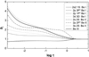 |
Fig. 3. Departure coefficients, bi, of different atomic levels of Be I and Be II in the solar atmosphere, plotted as a function of optical depth. |
Several factors may account for this difference with the earlier studies. First, the Be I and Be II stages of the Be model atom used in our study contain more atomic levels and thus allow the b–b and b–f transitions that involve the highest levels to be better accounted for. Second, we used the most up-to-date collisional rates with electrons and hydrogen obtained using quantum mechanical computations. In fact, quantum mechanical cross-sections of collisional ionisation by hydrogen from the first two levels of Be I obtained by Yakovleva et al. (2016) are two to five orders of magnitude lower than those predicted in the Drawin’s approximation. At the same time, the cross-sections of Yakovleva et al. (2016) are two to four orders of magnitude higher than in the Drawin’s approximation for the higher levels of Be I. Inevitably, this should lead to changes in the ionisation balance between Be I and Be II.
To verify the importance of the factors described above, we used the same 98-level model atom but with the collisional rates computed using the Drawin’s approximation (SH = 1). With this, we obtained an NLTE–LTE Be abundance correction of −0.035 dex. If the model atom is simplified further to consist of ten levels of Be I, five levels of Be II, the ground level of Be III, and collisional rates with electrons and hydrogen computed using van Regemorter’s and Drawin’s formulae, respectively, we obtain the abundance correction of −0.01 dex, which is in excellent agreement with those determined by Garcia Lopez et al. (1995) and Takeda et al. (2011). Repeating calculations with the 16-level model atom at several other combinations of Teff and log g, we obtain abundance corrections that agree very well with those of Takeda et al. (2011) (Table C.1). This leads us to the conclusion that the differences between the solar Be abundance obtained by us and other authors are due to the increased complexity and realism of our model atom.
Clearly, it is always desirable to check whether the NLTE abundances of a given element agree if they are determined from lines that form due to transitions from different multiplets in different ionisation stages. This, however, is not possible in the case of Be because the lines of Be I are located in the UV (234.8, 249.4, 265.0 nm) and are very heavily blended in the solar spectrum.
Finally, we recall that the missing UV opacity (Sect. 3.1) has a direct influence on the determined Be abundance. For example, using standard (i.e. uncorrected) ATLAS9 opacities and our new Be model atom, we obtain the solar Be abundance of A(Be)NLTE = 1.09 ± 0.05. By adding b–f opacities of Fe I and Fe II from the TURBOSPECTRUM package, as well as opacities resulting from the dissociation of CN and NH (C18), one obtains A(Be)NLTE = 1.18 ± 0.05. This value is 0.14 dex lower than that obtained by us with the adjusted Fe b–f opacities. One may anticipate that this effect will be important in other types of stars as well and thus has to be properly taken into account.
3.4. NLTE effects and Be abundances in stellar atmospheres
To estimate the influence of NLTE effects on the formation of Be II 313.04 and 313.11 nm resonance lines in the atmospheres of other types of stars, we computed a small grid of 1D NLTE–LTE Be abundance corrections. For this we used ATLAS9 model atmospheres with 4500 ≤ Teff ≤ 6500 K, 2.0 ≤ log g ≤ 5.0, −2.0 ≤ [Fe/H]≤ + 0.5, ξmicro = 2 km s−1, and [Be/Fe] = −0.5; 0.0; +0.5. Abundance corrections are provided in Fig. 4 and Table B.1.
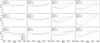 |
Fig. 4. 1D NLTE–LTE Be abundance corrections for the Be II 313.11 nm resonance line, for different values of Teff, log g, [Fe/H], and [Be/Fe]. |
Importantly, the obtained corrections show that NLTE effects may be substantial in other types of stars as well (Fig. 4). In extreme cases they may reach up to −0.3 dex, with a general tendency of corrections being larger at the lower effective temperatures and higher gravities. The correction may be positive or negative depending on which process – over-ionisation or over-excitation – dominates. There is also a clear dependence on the metallicity because collisions are less efficient at lower metallicities and thus NLTE deviations become larger. All this serves as a clear indication that NLTE effects have to be properly taken into account in Be abundance determinations.
Importantly, the Be abundance corrections are weakly sensitive to the effects of missing UV opacity. For example, the difference in the NLTE corrections for the Sun computed with and without taking the missing opacity into account is less than 0.015 dex. This is because the corrections measure only the relative effect on the determined abundance, not its absolute value. Clearly, the absolute 1D NLTE abundance will be affected if the missing opacity is not taken into account.
4. Conclusions
We studied the influence of NLTE effects on the formation of Be II 313.04 and 313.11 nm resonance lines in solar and stellar atmospheres. For this, we constructed a new model atom of Be using the most up-to-date atomic data obtained in recent years using quantum mechanical computations. We find that NLTE effects play an important role both in the solar and stellar atmospheres and, depending on the combination of stellar parameters, metallicity, and Be abundance, may lead to either the strengthening or weakening of Be II lines. As a consequence, the solar Be abundance obtained in this study, A(Be)NLTE = 1.32 ± 0.05, is slightly lower than the value obtained in earlier studies (cf. A(Be)NLTE = 1.38 ± 0.09 from Asplund et al. 2021) but is in excellent agreement with the meteoritic abundance determined by Lodders (2021), A(Be) = 1.31 ± 0.04. We also provide a grid of NLTE–LTE abundance corrections to aid future Be abundance studies in late-type stars.
We also show that one of the important problems in Be abundance determinations is missing opacity in the blue–UV spectral range. No opacity source has been identified as being capable of making the synthetic and observed solar fluxes agree in this wavelength range. Clearly, work on improving opacities in this spectral range is of utmost importance, not only for the Be abundance studies but also for those of other elements whose lines are located at 250 − 390 nm.
Acknowledgments
We thank the referee Martin Asplund for his extensive and constructive comments that helped to improve the paper significantly. Our study has benefited from the European Union’s Horizon 2020 research and innovation programme under grant agreement No 101008324 (ChETEC-INFRA). This work has made use of the VALD database, operated at Uppsala University, the Institute of Astronomy RAS in Moscow, and the University of Vienna.
References
- Allen, C. W. 1973, Astrophysical Quantities (London: University of London, Athlone Press) [Google Scholar]
- Ashwell, J. F., Jeffries, R. D., & Smalley, B. 2005, Mem. Soc. Astron. It. Suppl., 8, 206 [Google Scholar]
- Asplund, M. 2004, A&A, 417, 769 [NASA ADS] [CrossRef] [EDP Sciences] [Google Scholar]
- Asplund, M. 2005, ARA&A, 43, 481 [Google Scholar]
- Asplund, M., Amarsi, A. M., & Grevesse, N. 2021, A&A, 653, A141 [NASA ADS] [CrossRef] [EDP Sciences] [Google Scholar]
- Balachandran, S. C., & Bell, R. A. 1998, Nature, 392, 791 [NASA ADS] [CrossRef] [Google Scholar]
- Barklem, P. S., Piskunov, N., & O’Mara, B. J. 2000, A&AS, 142, 467 [NASA ADS] [CrossRef] [EDP Sciences] [Google Scholar]
- Bell, R. A., Balachandran, S. C., & Bautista, M. 2001, ApJ, 546, L65 [NASA ADS] [CrossRef] [Google Scholar]
- Carlberg, J. K., Cunha, K., Smith, V. V., & do Nascimento, J.-D., Jr. 2018, ApJ, 865, 8 [NASA ADS] [CrossRef] [Google Scholar]
- Carlsson, M. 1986, Upps. Astron. Obs. Rep., 33 [Google Scholar]
- Castelli, F., & Kurucz, R. L. 2003, in Modelling of Stellar Atmospheres, eds. N. Piskunov, W. W. Weiss, & D. F. Gray, 210, A20 [Google Scholar]
- Cunto, W., Mendoza, C., Ochsenbein, F., & Zeippen, C. J. 1993, A&A, 275, L5 [NASA ADS] [Google Scholar]
- Delgado Mena, E., Israelian, G., González Hernández, J. I., Santos, N. C., & Rebolo, R. 2012, ApJ, 746, 47 [NASA ADS] [CrossRef] [Google Scholar]
- Dipti, Das, T., Bartschat, K., et al. 2019, At. Data Nucl. Data Tables, 127, 1 [Google Scholar]
- Drawin, H.-W. 1968, Z. Phys., 211, 404 [NASA ADS] [CrossRef] [Google Scholar]
- Fontenla, J. M., Stancil, P. C., & Landi, E. 2015, ApJ, 809, 157 [NASA ADS] [CrossRef] [Google Scholar]
- Garcia Lopez, R. J., Severino, G., & Gomez, M. T. 1995, A&A, 297, 787 [NASA ADS] [Google Scholar]
- Holweger, H., & Mueller, E. A. 1974, Sol. Phys., 39, 19 [NASA ADS] [CrossRef] [Google Scholar]
- Korotin, S. A., Andrievsky, S. M., & Luck, R. E. 1999, A&A, 351, 168 [NASA ADS] [Google Scholar]
- Kramida, A., Ralchenko, Y., & Reader, J. 2012, APS Meeting Abstracts, 43, D1.004 [NASA ADS] [Google Scholar]
- Kurucz, R. L., Furenlid, I., Brault, J., & Testerman, L. 1984, Solar flux atlas from 296 to 1300 nm (Sunspot, New Mexico: National Solar Observatory) [Google Scholar]
- Lodders, K. 2021, Space Sci. Rev., 217, 44 [NASA ADS] [CrossRef] [Google Scholar]
- Meftah, M., Damé, L., Bolsée, D., et al. 2018, A&A, 611, A1 [NASA ADS] [CrossRef] [EDP Sciences] [Google Scholar]
- Mészáros, S., Allende Prieto, C., Edvardsson, B., et al. 2012, AJ, 144, 120 [Google Scholar]
- Plez, B. 2012, Astrophysics Source Code Library [record ascl:1205.004] [Google Scholar]
- Prantzos, N. 2012, A&A, 542, A67 [NASA ADS] [CrossRef] [EDP Sciences] [Google Scholar]
- Ryabchikova, T., Piskunov, N., Kurucz, R. L., et al. 2015, Phys. Scr., 90, 054005 [Google Scholar]
- Seaton, M. J. 1962, in Atomic and Molecular Processes, ed. D. R. Bates (New York: Academic Press) [Google Scholar]
- Smiljanic, R., Pasquini, L., Charbonnel, C., & Lagarde, N. 2010, A&A, 510, A50 [NASA ADS] [CrossRef] [EDP Sciences] [Google Scholar]
- Smiljanic, R., Zych, M. G., & Pasquini, L. 2021, A&A, 646, A70 [NASA ADS] [CrossRef] [EDP Sciences] [Google Scholar]
- Steenbock, W., & Holweger, H. 1984, A&A, 130, 319 [NASA ADS] [Google Scholar]
- Summers, H. P., & O’Mullane, M. G. 2011, in 7th International Conference on Atomic and Molecular Data and Their Applications – ICAMDATA-2010, eds. A. Bernotas, R. Karazija, & Z. Rudzikas, AIP Conf. Ser., 1344, 179 [Google Scholar]
- Tachiev, G., & Froese Fischer, C. 1999, J. Phys. B At. Mol. Phys., 32, 5805 [NASA ADS] [CrossRef] [Google Scholar]
- Takeda, Y., Tajitsu, A., Honda, S., et al. 2011, PASJ, 63, 697 [NASA ADS] [Google Scholar]
- Tsymbal, V., Ryabchikova, T., & Sitnova, T. 2019, in Physics of Magnetic Stars, eds. D. O. Kudryavtsev, I. I. Romanyuk, & I. A. Yakunin, ASP Conf. Ser., 518, 247 [NASA ADS] [Google Scholar]
- Tucci Maia, M., Meléndez, J., Castro, M., et al. 2015, A&A, 576, L10 [NASA ADS] [CrossRef] [EDP Sciences] [Google Scholar]
- van Regemorter, H. 1962, ApJ, 136, 906 [NASA ADS] [CrossRef] [Google Scholar]
- Woods, T. N., Prinz, D. K., Rottman, G. J., et al. 1996, J. Geophys. Res., 101, 9541 [NASA ADS] [CrossRef] [Google Scholar]
- Yakovleva, S. A., Voronov, Y. V., & Belyaev, A. K. 2016, A&A, 593, A27 [NASA ADS] [CrossRef] [EDP Sciences] [Google Scholar]
- Yan, Z.-C., Tambasco, M., & Drake, G. W. F. 1998, Phys. Rev. A, 57, 1652 [NASA ADS] [CrossRef] [Google Scholar]
Appendix A: List of spectral lines in the vicinity of Be II lines
As described in Sect. 3.2, in order to determine Be abundance in the Sun we adjusted the parameters of several spectral lines located in the immediate neighbourhood of Be II lines. The full line list in this spectral range is provided in Table A and includes all lines that were used in spectral synthesis calculations for the determination of solar Be abundance (i.e. lines with the modified line parameters and lines with the original line parameters from the VALD database). The lines for which parameters were modified in accordance to the description provided in Sect. 3.2 are marked in bold.
Parameters of spectral lines in the vicinity of Be II lines.
Appendix B: 1D NLTE–LTE abundance corrections for the Be II 313.11 nm line
The 1D NLTE–LTE abundance corrections for the Be II 313.11 nm line are provided in Table B.1. Effective temperatures and surface gravities are given in Cols. 1 and 2, respectively, and the remaining columns show abundance corrections for the Be II 313.11 nm line computed for different [Fe/H] and [Be/Fe] ratios.
1D NLTE–LTE abundance corrections for the Be II 313.11 nm line.
Appendix C: Comparison of NLTE–LTE abundance corrections for the Be II 313.11 nm line with those from Takeda et al. (2011)
One important finding of our study is that NLTE effects may strengthen the Be II resonance lines significantly, both in the Sun and other types of stars (Sects. 3.3 and 3.4), leading to significant NLTE–LTE abundance corrections (Sect. B). This is in contrast to what was found in earlier studies of Be NLTE abundances in the Sun (Sect. 3.3). As discussed in Sect. 3.3, we believe that the main reason for these differences is that the Be model atom used in our study consists of a significantly larger number of levels and transitions and uses the most up-to-date quantum mechanical data for treating the collisions with hydrogen (Sect. 3.3).
To assess how important these improvements could be for the realistic description of NLTE effects in Be line formation, we used a simplified model atom consisting of ten levels of Be I, five levels of Be II, and the ground level of Be III, with the collisional rates with electrons and hydrogen computed using the van Regemorter’s and Drawin’s formulae, respectively. With these assumptions, the simplified model atom loosely matches the complexity of the model atom used in, for example, the study of Takeda et al. (2011).
The obtained abundance corrections are provided in Table C.1, along with those obtained in the study of Takeda et al. (2011), and show that there is a very good agreement between the corrections obtained in the two studies: for Teff = 5500 and log g = 4.0 the difference is only −0.01 dex (ours versus theirs). Indeed, the differences between the corrections become significant if the full Be model atom is used in our calculations: for the same atmospheric parameters, we obtain the abundance correction of −0.08 dex, while Takeda et al. (2011) predict zero abundance correction.
Comparison of the NLTE–LTE abundance corrections for the Be II 313.11 nm line obtained in this study with those determined by Takeda et al. (2011).
Appendix D: Be abundance corrections for the most metal-poor stars
In their recent study of Be abundances in the most metal-poor Galactic stars, Smiljanic et al. (2021) suggested that at the lowest metallicity end the Be abundances may shown indications for the existence of ‘Be-plato’. Since the Be abundance corrections obtained in our study do show a tendency to increase with decreasing metallicity, one may therefore wonder how large NLTE effects may be in the most metal-poor Galactic stars. We therefore computed Be abundance corrections for the Be II 313.11 nm line for stars with various combinations of Teff and log g at [Fe/H] = −3.0. The results are provided in Table D.1 for cases where the equivalent width of the Be II 313.11 nm line is EW > 1 pm.
1D NLTE–LTE abundance corrections for the Be II 313.11 nm line at [Fe/H] = −3.0 (for cases with EW > 1 pm).
Clearly, for some combinations of stellar parameters and Be abundances, the abundance corrections may become significant. However, even in the most extreme cases this would not be sufficient to account for the ∼1 dex excess in Be abundances obtained in the LTE analysis of Smiljanic et al. at [Fe/H] ≤ −3.0.
All Tables
Comparison of the NLTE–LTE abundance corrections for the Be II 313.11 nm line obtained in this study with those determined by Takeda et al. (2011).
1D NLTE–LTE abundance corrections for the Be II 313.11 nm line at [Fe/H] = −3.0 (for cases with EW > 1 pm).
All Figures
|
Fig. 1. Synthetic and observed solar fluxes in the blue–UV spectral range. Top: comparison of synthetic fluxes with the observed SOLSPEC flux. Bottom: comparison of synthetic and observed CSIM and UARS fluxes. |
| In the text | |
|
Fig. 2. Observed solar spectrum from the Kurucz atlas (dots) and the best-fitted synthetic SynthV spectra (solid lines) in the vicinity of Be II lines. The solid blue line denotes a synthetic spectrum with the Be II lines computed in NLTE and the remaining lines in LTE. Solid red lines are Be II profiles computed in LTE with the same Be abundance. |
| In the text | |
|
Fig. 3. Departure coefficients, bi, of different atomic levels of Be I and Be II in the solar atmosphere, plotted as a function of optical depth. |
| In the text | |
|
Fig. 4. 1D NLTE–LTE Be abundance corrections for the Be II 313.11 nm resonance line, for different values of Teff, log g, [Fe/H], and [Be/Fe]. |
| In the text | |
Current usage metrics show cumulative count of Article Views (full-text article views including HTML views, PDF and ePub downloads, according to the available data) and Abstracts Views on Vision4Press platform.
Data correspond to usage on the plateform after 2015. The current usage metrics is available 48-96 hours after online publication and is updated daily on week days.
Initial download of the metrics may take a while.