© ESO 2021

1. Introduction

Plasma in galaxy clusters and groups is an almost completely ionized gas, is a generator of magnetic fields, and is subjected to turbulent motions. It is expected to thermalize after the accretion into the potential well on a timescale of the order of few gigayears, with a residual kinetic component whose distribution and total amplitude are still unknown.

In this Letter, we propose a modelization of this residual non-thermal pressure, which supports the gas in equilibrium within an assumed dark-matter gravitation field, and apply the suggested technique to the observed thermodynamic profiles recovered for the objects in our XMM-Newton Cluster Outskirts Project (X-COP) sample (Eckert et al. 2017). We build the relations between this non-thermal pressure and any magnetic fields and/or turbulent velocity in the plasma and determine how the non-thermal pressure translates into a hydrostatic bias on the mass measurement.

2. The hydrostatic equation, the non-thermal pressure, and the hydrostatic bias

Euler’s equation for an ideal fluid (i.e. a fluid in which thermal conductivity and viscosity do not play a relevant role) in a gravitational potential ϕ and with a velocity v, pressure P_gas, and density ρ_gas is (e.g., Landau & Lifshitz 1959; Suto et al. 2013)

$$\begin{array}{c}\hfill \frac{\partial \mathit{v}}{\partial t}+(\mathit{v}·\mathrm{\nabla })\mathit{v}=-\frac{1}{{\rho }_{\mathrm{gas}}}\mathrm{\nabla }{P}_{\mathrm{gas}}-\mathrm{\nabla }\varphi .\end{array}$$(1)

Lau et al. (2013), Nelson et al. (2014), and Biffi et al. (2016) discuss the relative role of the different contributors to the total potential, allowing the total mass, M_tot, to be written as the quantity that satisfies the following differential equation:

$$\begin{array}{c}\hfill \frac{1}{{\rho }_{\mathrm{gas}}}\frac{\mathrm{d}{P}_{\mathrm{tot}}}{\mathrm{d}r}=-\frac{\mathrm{d}\varphi }{\mathrm{d}r}=-\frac{G{M}_{\mathrm{tot}}}{r^2},\end{array}$$(2)

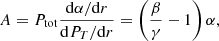
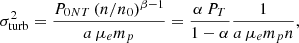
where G is the gravitational constant and P_tot = P_T + P_NT is the total pressure that we can express as the sum of the thermal component (P_T = P_gas = ρ_gas kT_gas/(μm_u) = n_gas kT_gas¹) and a non-thermal (not better defined) quantity, P_NT, that includes components generated from the velocity field, v, in Eq. (1) and accounts for: the rotational support due to mean tangential motions of gas; spatial variations in the mean radial streaming gas velocities; eventual correlations between the radial and tangential components of the random motions; and temporal variations in the mean radial gas velocities at a fixed radius. These temporal variations, also known as the acceleration bias, have been shown in Nelson et al. (2014) to be less than few per cent in relaxed systems but comparable to the effect induced from turbulent and bulk motions in disturbed ones, with a contribution that spans values between 40 and 20 per cent of the non-thermal pressure support moving outwards (see e.g., Biffi et al. 2016; Angelinelli et al. 2020).

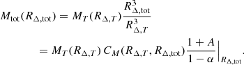
If we write the total mass as M_tot ∼ r²/n dP_tot/dr and the mass component due to the thermal-only pressure as M_T ∼ r²/n dP_T/dr, the following relation holds between the two

$$\begin{array}{c}\hfill M_{\mathrm{tot}}=M_T\frac{1+P_{\mathrm{tot}}(\mathrm{d}\alpha /\mathrm{d}r)/(\mathrm{d}{P}_T/\mathrm{d}r)}{1-\alpha }=M_T\frac{1+A}{1-\alpha },\end{array}$$(3)

where

$$\begin{array}{cc}& \alpha =\frac{P_{\mathit{NT}}}{P_{\mathrm{tot}}},\hfill \\ \hfill & A=P_{\mathrm{tot}}\frac{\mathrm{d}\alpha /\mathrm{d}r}{\mathrm{d}{P}_T/\mathrm{d}r}.\hfill \end{array}$$(4)

We can now link this expression to the hydrostatic bias, b, the correction needed to reconcile hydrostatic mass measurements with the expected ‘true’ value (see e.g., the reviews in Ettori et al. 2013; Pratt et al. 2019, for an extensive discussion on the measurements of b and their cosmological implications):

$$\begin{array}{c}\hfill M_{\mathrm{\Delta },T}=(1-b)M_{\mathrm{\Delta },\mathrm{tot}},\end{array}$$(5)

where we consider the estimates of the mass at a given overdensity 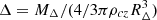$\mathrm{\Delta }=M_{\mathrm{\Delta }}/(4/3\pi {\rho }_{cz}{R}_{\mathrm{\Delta }}^3)$ with respect to the critical mass density at redshift z, 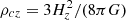${\rho }_{cz}=3H_z^2/(8\pi G)$, with H_z = H₀[Ω_m(1+z)³+1−Ω_m]^1/2 being the Hubble constant at that redshift in a flat Universe with Ω_m = 1 − Λ. All the measurements quoted in the present analysis have been made assuming H₀ = 70 km s⁻¹ Mpc⁻¹ and Ω_m = 0.3.

In general, the computation of Eq. (5) relies on the availability of M_Δ, T from X-ray measurements and M_Δ,tot from what is assumed to be a less biased true mass proxy, for example the one based on weak-lensing signals (e.g., Meneghetti et al. 2010). We note, however, that some assumptions have to be made on where (i.e. at which radius) the comparison is done to estimate b. If the mass is estimated at a given overdensity, Δ, or at the same physical radius, r, by combining Eqs. (3) and (5), we can write

$$\begin{array}{c}\hfill b=b(r)=\frac{\alpha (r)+A(r)}{1+A(r)},\end{array}$$(6)

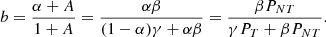
which becomes b = α when α is a constant (i.e. dα/dr = 0, and thus A = 0). Hereafter, we assume implicitly that b depends on radius. When needed, we will indicate to which radius (typically R₅₀₀) we are referring for some specific value of b. In the case under consideration, the mass values are estimated at the same physical radius (e.g., at the overdensity, Δ, for the total mass profile, M_tot, i.e. the radius R_Δ,tot), but only M_T(R_Δ, T) is known, and R_Δ,tot has to be inferred. Then, by definition, the following relation holds between M_Δ,tot = M_tot(R_Δ,tot) and M_Δ, T = M_T(R_Δ, T), $M_{\mathrm{\Delta },\mathrm{tot}}/R_{\mathrm{\Delta },\mathrm{tot}}^3=M_{\mathrm{\Delta },T}/R_{\mathrm{\Delta },T}^3$, allowing us to write

$$\begin{array}{cc}& M_{\mathrm{tot}}(R_{\mathrm{\Delta },\mathrm{tot}})=M_T(R_{\mathrm{\Delta },T})\frac{R_{\mathrm{\Delta },\mathrm{tot}}^3}{R_{\mathrm{\Delta },T}^3}\hfill \\ \hfill & =M_T(R_{\mathrm{\Delta },T})C_M(R_{\mathrm{\Delta },T},R_{\mathrm{\Delta },\mathrm{tot}})\frac{1+A}{1-\alpha }{|}_{R_{\mathrm{\Delta },\mathrm{tot}}}.\hfill \end{array}$$(7)

Under the assumption that we measure M_T(R_Δ, T), the hydrostatic bias is estimated as 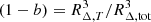$(1-b)=R_{\mathrm{\Delta },T}^3/R_{\mathrm{\Delta },\text{tot}}^3$ or (1 − b) = (1 − α)/(1 + A)|_RΔ, tot/C_M(R_Δ, T, R_Δ, tot), where C_M(R_Δ, T, R_Δ, tot) is the ratio between the ‘thermal’ mass evaluated at R_Δ, tot and at R_Δ, T, which can be evaluated for a given mass profile of f(r) = M_T(r)/M_T0 as C_M(R_Δ, T, R_Δ, tot) = f(R_Δ, tot)/f(R_Δ, T).

3. Modeling the non-thermal pressure

In this section we investigate how these calculations can be done by adopting some functional forms for P_T and P_NT.

As we have shown in Ghirardini et al. (2019b), a polytropic function, with an effective polytropic index γ, is a very good representation for the thermal gas distribution: P_T = P_0T (n/n₀)^γ. Given our ignorance on the true, and probably not univocal, origin of the non-thermal pressure (apart from speculations based on hydrodynamical simulations in e.g., Shi & Komatsu 2014; Nelson et al. 2014; Angelinelli et al. 2020), we continue to adopt the thermal electronically charged gas distribution as a proxy for its distribution: P_NT = P_0NT (n/n₀)^β. Then,

$$\begin{array}{c}\hfill \alpha =\frac{P_{\mathit{NT}}}{P_{\mathrm{tot}}}={[\frac{P_{0T}}{P_{0NT}}{\left(\frac{n}{n_0}\right)}^{\gamma -\beta }+1]}^{-1}\end{array}$$(8)

$$\begin{array}{c}\hfill A=P_{\mathrm{tot}}\frac{\mathrm{d}\alpha /\mathrm{d}r}{\mathrm{d}{P}_T/\mathrm{d}r}=(\frac{\beta }{\gamma }-1)\alpha ,\end{array}$$(9)

where we have made use of the following relations: dP_T/dr = P_0Tγn^γ − 1dn/dr and dP_NT/dr = P_0NTβn^β − 1dn/dr.

As final step, we can now also rewrite the hydrostatic bias in Eq. (6) as

$$\begin{array}{c}\hfill b=\frac{\alpha +A}{1+A}=\frac{\alpha \beta }{(1-\alpha )\gamma +\alpha \beta }=\frac{\beta P_{\mathit{NT}}}{\gamma P_T+\beta P_{\mathit{NT}}}.\end{array}$$(10)

Again, when dα/dr = 0, then γ = β, and b = P_NT/(P_T + P_NT) = α. For physical reasons, α ≥ 0 and γ > 0. Then, b ≥ 0 only when β ≥ 0. If dα/dr ≠ 0, then we have a complete modelization of the radial behaviour of the hydrostatic bias, b.

To constrain the non-thermal component, Shi et al. (2016) propose adopting an analytic model (described in Shi & Komatsu 2014) that is able to predict the amplitude of non-thermal pressure and its radial, mass, and redshift dependences, but only once the mass accretion history of the cluster is known. Alternatively, and under the common condition that thermodynamic profiles based on only X-rays and Sunayev-Zel’dovich (SZ; Sunyaev & Zel’dovich 1972) effect are available, some external information on the total gravitational potential is needed. For instance, the total mass profiles can be derived from gravitational lensing data (see e.g., Sayers et al. 2021) or from stellar kinematics (as in early-type galaxies; see e.g., Churazov et al. 2008; Humphrey et al. 2013). Fusco-Femiano & Lapi (2013) fix the gas fraction at the viral radius equal to the cosmic baryon fraction, with the contribution from stars subtracted, to model any extra contribution in pressure given X-ray derived profiles. To account for the complex physical processes that can affect the relative distributions of the baryons in a cosmological contest, we (Ghirardini et al. 2018; Eckert et al. 2019) propose using a ‘universal’ gas fraction, f_g, U, derived from a mean baryon fraction measured at some given overdensities (typically Δ = 500 and 200) in massive haloes extracted from hydrodynamical simulations and hence corrected for a statistical contribution of the stellar fraction (i.e. f_g, U = f_b, sims − f_star, stat). In the following analysis, we adopt the measurements of this universal gas fraction presented and discussed in our previous work (see e.g., Sect. 3.1 in Eckert et al. 2019): f_g, U(R₅₀₀) = 0.131 ± 0.009 and f_g, U(R₂₀₀) = 0.134 ± 0.007. We discuss below the impact of this assumption on our constraints of the non-thermal pressure.

In Eckert et al. (2019), a model for α (instead of P_NT) – presented in Nelson et al. (2014) as a simple, not physically motivated, universal functional form of the radial behaviour observed in cosmological hydrodynamical simulations – is adopted and solved iteratively in its two free parameters (a third scale parameter is maintained fixed). In the present work, we suggest adopting a modelization of the non-thermal pressure as directly proportional to the electron density – which is more physically plausible since the electron density is the natural reservoir of the magnetic fields and particles to be accelerated – and with model parameters that are more easily interpretable as physical quantities.

The total true mass is then recovered by comparing f_g, U to the observed f_g, T, which is based on the ‘thermal-only’ gravitational mass profile (described in Ettori et al. 2019) and on the gas mass profile previously corrected for some gas clumping that might bias the gas density reconstruction (see the discussion on the recovered thermodynamic profiles in Ghirardini et al. 2019a and Sect. 5.1 in Eckert et al. 2019 on the systematic uncertainties affecting f_g, T). By propagating the hydrostatic bias in Eqs. (5) and (6), we can write

$$\begin{array}{c}\hfill f_g=\frac{M_g}{M_{\mathrm{tot}}}{|}_{R_{\mathrm{\Delta },\mathrm{tot}}}=\frac{M_{g,T}}{M_T}{|}_{R_{\mathrm{\Delta },\mathrm{tot}}}\frac{1-\alpha }{1+A}{|}_{R_{\mathrm{\Delta },\mathrm{tot}}}.\end{array}$$(11)

We note that the gas fraction will be evaluated at two different radii, R_Δ, tot and R_Δ, T, which correspond to the true and thermal-only mass profile, respectively. With only R_Δ, T known from direct observations (R_Δ, tot depends on the mass profile corrected for the hydrostatic bias), we compute all these quantities at R_Δ, T and write

$$\begin{array}{cc}& \frac{M_g}{M_{\mathrm{tot}}}{|}_{R_{\mathrm{\Delta },T}}=f_g{|}_{R_{\mathrm{\Delta },\mathrm{tot}}}{C}_f(R_{\mathrm{\Delta },\mathrm{tot}},R_{\mathrm{\Delta },T})\hfill \\ \hfill & =f_{g,T}{|}_{R_{\mathrm{\Delta },T}}\frac{1-\alpha }{1-\alpha (\gamma -\beta )/\gamma }{|}_{R_{\mathrm{\Delta },T}}.\hfill \end{array}$$(12)

In this equation: f_g|_RΔ, tot is extracted from hydrodynamical simulations; f_g, T|_RΔ, T and γ are measured from the observations; and α and β are the unknowns.

The correction factor C_f(R_Δ, tot, R_Δ, T) = f_g(R_Δ, T)/f_g(R_Δ, tot) used to convert the gas fraction from numerical simulations at different radii can be estimated by assuming that n ∼ r^−ϵ in the region of interest (around R₅₀₀ and R₂₀₀). Then, M_g(R_Δ, T)/M_g(R_Δ, tot) = (R_Δ, T/R_Δ, tot)^3 − ϵ, and, using Eq. (7), C_f = f_g(R_Δ, T)/f_g(R_Δ, tot)≈(R_Δ, T/R_Δ, tot)^3 − ϵ × C_M(R_Δ, T, R_Δ, tot). Moreover, by assuming the power-law behaviour of n and P, and applying the HE to M_T and M_tot as in Eq. (3), we obtain that

$$\begin{array}{cc}& M_T=r^{1+ϵ-ϵ\gamma }\hfill \\ \hfill & M_{\mathrm{tot}}=r^{1+ϵ-ϵ\gamma }(1+\frac{\beta }{\gamma }\frac{P_{0NT}}{P_{0T}}{r}^{\gamma ϵ-\beta ϵ}),\hfill \end{array}$$(13)

which can be used to estimate C_M(R_Δ, T, R_Δ, tot) = M_tot(R_Δ, tot) / M_tot(R_Δ, T). Using the relation between R_Δ, tot and R_Δ, T (see Eq. (7)) with Eq. (13), we can then write

$$\begin{array}{c}\hfill R_{\mathrm{\Delta },T}^{ϵ-\gamma ϵ-2}=R_{\mathrm{\Delta },\mathrm{tot}}^{ϵ-\gamma ϵ-2}(1+\frac{\beta }{\gamma }\frac{P_{0NT}}{P_{0T}}{R}_{\mathrm{\Delta },\mathrm{tot}}^{\gamma ϵ-\beta ϵ})\end{array}$$(14)

and, finally,

$$\begin{array}{c}\hfill C_f=\frac{f_g(R_{\mathrm{\Delta },T})}{f_g(R_{\mathrm{\Delta },\mathrm{tot}})}={\left(\frac{R_{\mathrm{\Delta },T}}{R_{\mathrm{\Delta },\mathrm{tot}}}\right)}^{-ϵ}{(1+\frac{\beta }{\gamma }\frac{P_{0NT}}{P_{0T}}{R}_{\mathrm{\Delta },T}^{\gamma ϵ-\beta ϵ})}^{-1}.\end{array}$$(15)

In the present analysis, because we do not use the profiles in numerical simulations, we assume C_f = 1.

Considering that we know (i) the gas fraction, both the true and universal one, f_g, U, and the observed thermal one, f_g, T, at (at least) two given points (R₅₀₀ and R₂₀₀, from the thermal mass profile, M_T), (ii) the gas density, n, and (iii) a (mean) polytropic index, γ, in that radial range, we can estimate α and β, measuring both the normalization P_0NT and the radial dependence of the modelled P_NT. In details, if we define F₁ = f_g, U/f_g, T|_r1, F₂ = f_g, U/f_g, T|_r2, and $\gamma =\widehat{\gamma }$ as estimated from the recovered density and pressure profiles, and if we assume that the unknowns p₀ = P_0T/P_0NT and β do not vary with radius (though this assumption can also be relaxed once more measurements of F_i are available), we can write ${\alpha }_i=P_{\mathit{NT}}/P_{\mathrm{tot}}{|}_{r_i}={[p_0{(n_i/n_0)}^{\widehat{\gamma }-\beta }+1]}^{-1}$ and the following system of two equations with the two unknowns:

$$\begin{array}{c}\hfill \{\begin{array}{c}{F}_1=\frac{1-{\alpha }_1}{1+{\alpha }_1(\beta -\widehat{\gamma })/\widehat{\gamma }}\hfill \\ F_2=\frac{1-{\alpha }_2}{1+{\alpha }_2(\beta -\widehat{\gamma })/\widehat{\gamma }}.\hfill \end{array}\end{array}$$(16)

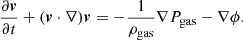
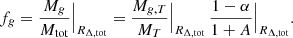
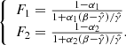
We note that the impact of the assumption on the value of f_g, U at a given radius can be easily quantified from Eq. (16). We represent this function by plotting in Fig. 1 how α varies as a function of β for different measurements of the effective polytropic index, γ, and of the ratios between the expected and the observed gas mass fraction, F. As expected, α increases as F decreases, for example by assuming lower values of the universal gas fraction, f_g, U, for a given measured f_g, T. Estimates of α between 0 and 1 are obtainable for any β only when F < 1, with α → 0 when F → 1. For values of F > 1, α will be larger than zero only when β < γ(F − 1)/F.

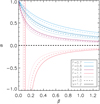Fig. 1. Representation of Eq. (16) in the form α = (1 − F)/[1+F(β−γ)/γ] for different values of F = fg, U/fg, T and of the effective polytropic index, γ.

By dividing F₁ by F₂, we can solve for p₀, included in α_i, as a function of β and after some math obtain

$$\begin{array}{c}\hfill p_0=\frac{\beta }{\widehat{\gamma }}[{\left(\frac{n_1}{n_2}\right)}^{\widehat{\gamma }-\beta }-\frac{F_1}{F_2}]{\left(\frac{n_1}{n_0}\right)}^{\beta -\widehat{\gamma }}{(\frac{F_1}{F_2}-1)}^{-1}.\end{array}$$(17)

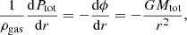
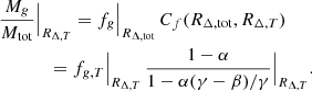
Then, we solve numerically using an array of values for β and by inserting Eq. (17) into the second term of one of the two equations in Eq. (16), as represented in Fig. 2. We present the results for the X-COP objects in Table 1. All our estimates are consistent with the results presented in Eckert et al. (2019). For five clusters, the constraints on α are consistent with zero: three of them have an estimated F_i > 1 at R₅₀₀ and/or R₂₀₀, implying a negative hydrostatic bias.

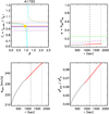Fig. 2. Example of the analysis applied to A1795. Upper left: distribution of the ratio of the expected gas fraction (the dashed orange line represents R500 and dashed cyan R200) and observed gas fraction, Fi (solid horizontal lines, with errors represented by dotted lines; red represents R500 and blue R200) as a function of the slope, β (see Eq. (16)); the best-fit value is indicated by the yellow dot. Upper right: distribution of α as a function of radius with, overplotted in purple, the prediction from the model of αturb in Angelinelli et al. (2020) and the expectations on the level of turbulence assuming η = 1/3 (green dashed line) and magnetic energy CE = 0.05 (green dotted line; see Sect. 4 for details). Lower left: distribution of the turbulent velocity as a function of radius (see Eq. (22)). Lower right: distribution of the relative energy (Eq. (23)) as a function of radius. In red, we show the region used to constrain γ; R500 and R200 are indicated with vertical dashed and dotted lines.

We note that our algorithm allows the radial behaviour of α to be constrained without any assumptions on the underlying functional form (such as those suggested from recent numerical simulations; see e.g., Shaw et al. 2010; Nelson et al. 2014; Angelinelli et al. 2020) and on a single object basis, although a universal mean gas fraction has to be imposed on all the systems.

4. Discussion on the interpretation of P_NT

The properties of the intracluster plasma are regulated through the action of cosmological supersonic flows, which accrete mass onto the cluster halo and inject energy that is then dissipated over different scales and under different forms, including non-thermal plasma components such as relativistic particles and magnetic fields (see e.g., Brunetti & Jones 2014). Miniati & Beresnyak (2015) present evidence from numerical simulations that the energy components follow a hierarchy that can be represented through some general relations between thermal energy, E_T, energy in turbulence, E_turb, and energy in magnetic field E_B = B²/(8π):

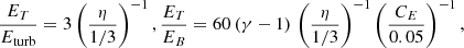$$\begin{array}{c}\hfill \frac{E_T}{E_{\mathrm{turb}}}=3{\left(\frac{\eta }{1/3}\right)}^{-1},\frac{E_T}{E_B}=60(\gamma -1){\left(\frac{\eta }{1/3}\right)}^{-1}{\left(\frac{C_E}{0.05}\right)}^{-1},\end{array}$$(18)

where η is the fraction of thermal energy originating from turbulent dissipation and C_E is the fraction of turbulent (kinetic) energy that converts into magnetic energy; η and C_E have expected values of about 1/3 and 0.05, respectively.

From the above equations, we can write that the magnetic field, B, is related to the thermal pressure, P_T, as

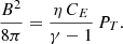$$\begin{array}{c}\hfill \frac{B^2}{8\pi }=\frac{\eta C_E}{\gamma -1}{P}_T.\end{array}$$(19)

Using the polytropic law for P_T = P_0T(n/n₀)^γ, we can then write B = (8π η C_E P_0T)^0.5(γ − 1)^−0.5(n/n₀)^γ/2 = B₀(n/n₀)^γ_B. With this modelization, we estimate a median B₀ of about 15 μG at 100 kpc. Furthermore, we can write the magnetic pressure as a fraction of the total pressure as

$$\begin{array}{c}\hfill \frac{P_B}{P_{\mathrm{tot}}}=\frac{\eta C_E/(\gamma -1)P_T}{P_T+P_{\mathit{NT}}}=\frac{\eta C_E/(\gamma -1)P_T}{P_T+\eta P_T}=\frac{\eta C_E}{(\gamma -1)(1+\eta )}.\end{array}$$(20)

In the extreme case that the entire non-thermal pressure support is in the form of turbulence, then P_NT = E_turb and η = P_NT/P_T = α/(1 − α), or α = η/(η + 1), which we overplot as a dashed green line in Fig. 2 for η = 1/3. We indicate the fraction of magnetic energy for C_E = 0.05 with a dotted green line. From our dataset of measurements of α(R₅₀₀), by requiring that P_B ≡ P_NT, we obtain median (mean) values of η of about 0.15 (0.3) and C_E, from the inversion of Eq. (20), ∼0.19 (0.16), with the former being more than half of, and the latter three to four times larger than, the estimates from numerical simulations.

Finally, if we convert P_NT into the velocity dispersion associated with the turbulence of the intracluster medium (ICM), we can write

$$\begin{array}{c}\hfill P_{\mathit{NT}}=a\rho {\sigma }_{\mathrm{turb}}^2=a{\mu }_e{m}_{p}n{\sigma }_{\mathrm{turb}}^2,\end{array}$$(21)

which implies

$$\begin{array}{c}\hfill {\sigma }_{\mathrm{turb}}^2=\frac{P_{0NT}{(n/n_0)}^{\beta -1}}{a{\mu }_e{m}_p}=\frac{\alpha P_T}{1-\alpha }\frac{1}{a{\mu }_e{m}_{p}n},\end{array}$$(22)

where a = 1/3 and 1 for the isotropic value and the radial component only, respectively, and ρ is the gas mass density equal to μ_em_pn (e.g., Vazza et al. 2018; Angelinelli et al. 2020). Similar treatment for the determination of the non-thermal pressure support is discussed in Humphrey et al. (2013), where the constraints from stellar dynamics are used to provide an unbiased estimate of the true gravitational potential in elliptical galaxies.

With the thermal velocity dispersion defined as ${\sigma }_{\text{th}}^2=k_{\text{B}}T/(a{\mu }_e{m}_p)=P_T/(a{\mu }_e{m}_{p}n)$, we can write the ratio between the turbulent velocity dispersion and the velocity dispersion produced by thermal motions as

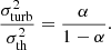$$\begin{array}{c}\hfill \frac{{\sigma }_{\mathrm{turb}}^2}{{\sigma }_{\mathrm{th}}^2}=\frac{\alpha }{1-\alpha }.\end{array}$$(23)

Inverting this equation, we can write the hydrostatic bias as a function of the turbulent velocity,

$$\begin{array}{c}\hfill b={(\frac{{\sigma }_{\mathrm{th}}^2}{{\sigma }_{\mathrm{turb}}^2}+1)}^{-1}.\end{array}$$(24)

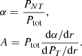
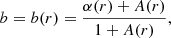
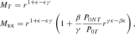
We used published values of upper limits on σ_turb to reconstruct the expected upper limits on b (from Eq. (24), b decreases as σ_turb decreases). In Fig. 3, we show the 𝒩(< b)−b (or hydrostatic bias density) distribution based on the constraints presented in Sanders et al. (2011) and Pinto et al. (2015) and obtained from the width of emission lines in XMM-Newton Reflection Grating Spectrometer spectra extracted from the inner regions of a sample of 62 galaxy clusters, groups, and elliptical galaxies and the 44 nearby, bright objects in the CHEERS sample, respectively. We note that the upper limits on b are larger in cooler systems. Limiting our analysis to the clusters with kT > 2 keV, and interpolating the distribution measured in the hotter systems of the CHEERS sample, we estimate upper limits on b < (0.33, 0.19, 0.09) in 80, 50, and 20 per cent of the population. Considering that these measurements are limited to the cluster’s cores, we estimated a median correction on the bias b, estimated at different radii, in the X-COP sample (see inset in Fig. 3) and obtain b(0.1R₅₀₀)≈0.5b(R₅₀₀), with a general increase in the bias moving outwards. Applying this correction to the upper limits in Pinto et al. (2015), we evaluate b < (0.64, 0.41, 0.20) in 80, 50, and 20 per cent of the population, respectively.

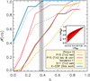Fig. 3. Density distribution of the hydrostatic bias, b. The values of b are inferred from Eq. (10), using the values tabulated in Table 1, for the X-COP objects at R500 (solid line) and at R200 (dotted line), and from Eq. (24) for the upper limits for the clusters in Pinto et al. (2015) (16 out of 44 with T > 2 keV; upper limits estimated within 0.8 arcmin) and Sanders et al. (2011) (36 out of 62). The purple line shows the constraints that include the correction to extrapolate the estimates from the core to R500 (see text and the inset, where we plot median distribution, with first and third quartiles, of the hydrostatic bias in the X-COP sample as a function of radius). The shaded region shows the constraints obtained from the Planck Collaboration by combining the cosmic microwave background anisotropies and the cluster number count (Planck Collaboration VI 2020).

We can now compare these upper limits with the results we obtain for the X-COP sample (see Fig. 3). The distribution of the bias in our objects covers lower values of b (with 80% of the objects with b < 0.17 and 50% with b < 0.03 at R₅₀₀), confirming that our bright local systems are, on average, relaxed (i.e. closer to the assumption of a spherically symmetric gas distribution in hydrostatic equilibrium with the underlying gravitational potential), as they were selected at origin. Three objects studied in our work are also present in Pinto et al. (2015). From the 1 σ upper limits quoted there, we infer that b = α from turbulence of about < 11%, < 51%, and < 29% for A85, A1795, and A2029, respectively, Only for A85 does this value appear to be similar to the constraints presented in Table 1; for A2029 and A1795, the levels of bias induced from the current upper limits are more than two and seven times the constraints we obtain.

Overall, these distributions of the hydrostatic bias, b, at R₅₀₀ are in good agreement with the mean values of about 10–20 per cent obtained in hydrodynamical simulations of massive haloes in a cosmological context (see e.g., Biffi et al. 2016; Pearce et al. 2020).

5. Conclusions

We have presented a new model of the non-thermal pressure as P_NT = P_0NT (n/n₀)^β and have applied it to the X-COP results on the radial profiles of the gas density, temperature, and pressure to constrain the parameters P_0NT and β. We converted this non-thermal pressure support to the bias b that affects the reconstruction of the mass profile through the hydrostatic equilibrium equation. We also translated P_NT into expected contributions in the form of magnetic fields and turbulent velocity in the ICM. Regarding turbulent velocity, we put interesting constraints on the expected distribution of the hydrostatic bias using upper limits on the turbulent velocities available in the literature. We propose the hydrostatic bias density distribution 𝒩(< b)−b as a way to assess statistically interesting and useful quantities that have an impact on the use of galaxy clusters for astrophysical and cosmological purposes. We show that current constraints (both upper limits on the turbulent velocity in the ICM and measurements from the gas mass fraction in X-COP; see Fig. 3) suggest that most of the studied galaxy clusters have a b lower than (or marginally consistent with, when the upper limits extrapolated up to R₅₀₀ are considered) the value of b = 0.38(±0.03) required to reconcile the measurements of the cosmic microwave background anisotropies with the SZ-based cluster number count from Planck data (Planck Collaboration VI 2020). We note that to accommodate for this value of b with the median estimates of β (0.84) and γ (1.19) recovered in the X-COP sample, by using Eqs. (10) and (16) and the measured f_g, T, we require f_g, U(R₅₀₀) to be 62% of the adopted value of 0.13 (i.e. a universal gas fraction of about 0.08). This value is more typical for 10¹⁴ M_⊙ systems, where the action of feedback has a larger impact than in more massive, X-COP-like, objects on the expected distribution of baryons, at least as it is resolved in state-of-the-art cosmological hydrodynamical simulations (see e.g., Fig. 15 in Eckert et al. 2021).

Future X-ray instruments with improved spectral resolution (e.g., XRISM² and X-IFU³ on board Athena⁴) will tighten these limits, providing significant constraints on the turbulent velocity and allowing the picture of the energy and mass budget of galaxy clusters to be completed. In the meantime, projects such as CHEX-MATE⁵ will provide a direct measurement of b by combining different mass proxies in an SZ-selected representative sample of galaxy clusters.

Acknowledgments

We thank the referee for some valuable comments. S.E. acknowledges financial contribution from the contracts ASI-INAF Athena 2019-27-HH.0, “Attività di Studio per la comunità scientifica di Astrofisica delle Alte Energie e Fisica Astroparticellare” (Accordo Attuativo ASI-INAF n. 2017-14-H.0), INAF mainstream project 1.05.01.86.10, and from the European Union’s Horizon 2020 Programme under the AHEAD2020 project (grant agreement n. 871158).

References

All Tables

All Figures

	Fig. 1. Representation of Eq. (16) in the form α = (1 − F)/[1+F(β−γ)/γ] for different values of F = fg, U/fg, T and of the effective polytropic index, γ.
In the text

Fig. 2. Example of the analysis applied to A1795. Upper left: distribution of the ratio of the expected gas fraction (the dashed orange line represents R500 and dashed cyan R200) and observed gas fraction, Fi (solid horizontal lines, with errors represented by dotted lines; red represents R500 and blue R200) as a function of the slope, β (see Eq. (16)); the best-fit value is indicated by the yellow dot. Upper right: distribution of α as a function of radius with, overplotted in purple, the prediction from the model of αturb in Angelinelli et al. (2020) and the expectations on the level of turbulence assuming η = 1/3 (green dashed line) and magnetic energy CE = 0.05 (green dotted line; see Sect. 4 for details). Lower left: distribution of the turbulent velocity as a function of radius (see Eq. (22)). Lower right: distribution of the relative energy (Eq. (23)) as a function of radius. In red, we show the region used to constrain γ; R500 and R200 are indicated with vertical dashed and dotted lines.

In the text

Fig. 3. Density distribution of the hydrostatic bias, b. The values of b are inferred from Eq. (10), using the values tabulated in Table 1, for the X-COP objects at R500 (solid line) and at R200 (dotted line), and from Eq. (24) for the upper limits for the clusters in Pinto et al. (2015) (16 out of 44 with T > 2 keV; upper limits estimated within 0.8 arcmin) and Sanders et al. (2011) (36 out of 62). The purple line shows the constraints that include the correction to extrapolate the estimates from the core to R500 (see text and the inset, where we plot median distribution, with first and third quartiles, of the hydrostatic bias in the X-COP sample as a function of radius). The shaded region shows the constraints obtained from the Planck Collaboration by combining the cosmic microwave background anisotropies and the cluster number count (Planck Collaboration VI 2020).

In the text

References

- Angelinelli, M., Vazza, F., Giocoli, C., et al. 2020, MNRAS, 495, 864 [NASA ADS] [CrossRef] [Google Scholar]
- Biffi, V., Borgani, S., Murante, G., et al. 2016, ApJ, 827, 112 [NASA ADS] [CrossRef] [Google Scholar]
- Brunetti, G., & Jones, T. W. 2014, Int. J. Mod. Phys. D, 23, 1430007 [Google Scholar]
- Churazov, E., Forman, W., Vikhlinin, A., et al. 2008, MNRAS, 388, 1062 [Google Scholar]
- Eckert, D., Ettori, S., Pointecouteau, E., et al. 2017, Astron. Nachr., 338, 293 [Google Scholar]
- Eckert, D., Ghirardini, V., Ettori, S., et al. 2019, A&A, 621, A40 [NASA ADS] [CrossRef] [EDP Sciences] [Google Scholar]
- Eckert, D., Gaspari, M., Gastaldello, F., Le Brun, A. M. C., & O’Sullivan, E. 2021, Universe, 7, 142 [NASA ADS] [CrossRef] [Google Scholar]
- Ettori, S., Donnarumma, A., Pointecouteau, E., et al. 2013, Space Sci. Rev., 177, 119 [Google Scholar]
- Ettori, S., Ghirardini, V., Eckert, D., et al. 2019, A&A, 621, A39 [NASA ADS] [CrossRef] [EDP Sciences] [Google Scholar]
- Fusco-Femiano, R., & Lapi, A. 2013, ApJ, 771, 102 [NASA ADS] [CrossRef] [Google Scholar]
- Ghirardini, V., Ettori, S., Eckert, D., et al. 2018, A&A, 614, A7 [NASA ADS] [CrossRef] [EDP Sciences] [Google Scholar]
- Ghirardini, V., Ettori, S., Eckert, D., & Molendi, S. 2019a, A&A, 627, A19 [NASA ADS] [CrossRef] [EDP Sciences] [Google Scholar]
- Ghirardini, V., Eckert, D., Ettori, S., et al. 2019b, A&A, 621, A41 [NASA ADS] [CrossRef] [EDP Sciences] [Google Scholar]
- Humphrey, P. J., Buote, D. A., Brighenti, F., Gebhardt, K., & Mathews, W. G. 2013, MNRAS, 430, 1516 [NASA ADS] [CrossRef] [Google Scholar]
- Landau, L. D., & Lifshitz, E. M. 1959, Fluid Mechanics (Pergamon Press) [Google Scholar]
- Lau, E. T., Nagai, D., & Nelson, K. 2013, ApJ, 777, 151 [NASA ADS] [CrossRef] [Google Scholar]
- Meneghetti, M., Rasia, E., Merten, J., et al. 2010, A&A, 514, A93 [NASA ADS] [CrossRef] [EDP Sciences] [Google Scholar]
- Miniati, F., & Beresnyak, A. 2015, Nature, 523, 59 [NASA ADS] [CrossRef] [Google Scholar]
- Nelson, K., Lau, E. T., & Nagai, D. 2014, ApJ, 792, 25 [NASA ADS] [CrossRef] [Google Scholar]
- Pearce, F. A., Kay, S. T., Barnes, D. J., Bower, R. G., & Schaller, M. 2020, MNRAS, 491, 1622 [NASA ADS] [CrossRef] [Google Scholar]
- Pinto, C., Sanders, J. S., Werner, N., et al. 2015, A&A, 575, A38 [NASA ADS] [CrossRef] [EDP Sciences] [Google Scholar]
- Planck Collaboration VI. 2020, A&A, 641, A6 [NASA ADS] [CrossRef] [EDP Sciences] [Google Scholar]
- Pratt, G. W., Arnaud, M., Biviano, A., et al. 2019, Space Sci. Rev., 215, 25 [Google Scholar]
- Sanders, J. S., Fabian, A. C., & Smith, R. K. 2011, MNRAS, 410, 1797 [NASA ADS] [Google Scholar]
- Sayers, J., Sereno, M., Ettori, S., et al. 2021, MNRAS, 505, 4338 [NASA ADS] [CrossRef] [Google Scholar]
- Shaw, L. D., Nagai, D., Bhattacharya, S., & Lau, E. T. 2010, ApJ, 725, 1452 [NASA ADS] [CrossRef] [Google Scholar]
- Shi, X., & Komatsu, E. 2014, MNRAS, 442, 521 [NASA ADS] [CrossRef] [Google Scholar]
- Shi, X., Komatsu, E., Nagai, D., & Lau, E. T. 2016, MNRAS, 455, 2936 [NASA ADS] [CrossRef] [Google Scholar]
- Sunyaev, R. A., & Zel’dovich, Y. B. 1972, Comments Astrophys. Space Phys., 4, 173 [Google Scholar]
- Suto, D., Kawahara, H., Kitayama, T., et al. 2013, ApJ, 767, 79 [NASA ADS] [CrossRef] [Google Scholar]
- Vazza, F., Angelinelli, M., Jones, T. W., et al. 2018, MNRAS, 481, L120 [NASA ADS] [CrossRef] [Google Scholar]