| Issue |
A&A
Volume 657, January 2022
|
|
|---|---|---|
| Article Number | A117 | |
| Number of page(s) | 12 | |
| Section | The Sun and the Heliosphere | |
| DOI | https://doi.org/10.1051/0004-6361/202141552 | |
| Published online | 20 January 2022 | |
Validation scheme for solar coronal models: Constraints from multi-perspective observations in EUV and white light
1
Institute of Physics, University of Graz, Universitätsplatz 5, 8010 Graz, Austria
e-mail: This email address is being protected from spambots. You need JavaScript enabled to view it.
2
Department of Physics, University of Helsinki, Gustaf Hällströmin katu 2, 00560 Helsinki, Finland
3
Max-Planck Institut für Sonnensystemforschung, Justus-von-Liebig Weg 3, 37077 Göttingen, Germany
Received:
15
June
2021
Accepted:
4
October
2021
Abstract
Context. In this paper, we present a validation scheme to investigate the quality of coronal magnetic field models, which is based on comparisons with observational data from multiple sources.
Aims. Many of these coronal models may use a range of initial parameters that produce a large number of physically reasonable field configurations. However, that does not mean that these results are reliable and comply with the observations. With an appropriate validation scheme, which is the aim of this work, the quality of a coronal model can be assessed.
Methods. The validation scheme was developed with the example of the EUropean Heliospheric FORecasting Information Asset (EUHFORIA) coronal model. For observational comparison, we used extreme ultraviolet and white-light data to detect coronal features on the surface (open magnetic field areas) and off-limb (streamer and loop) structures from multiple perspectives (Earth view and the Solar Terrestrial Relations Observatory – STEREO). The validation scheme can be applied to any coronal model that produces magnetic field line topology.
Results. We show its applicability by using the validation scheme on a large set of model configurations, which can be efficiently reduced to an ideal set of parameters that matches best with observational data.
Conclusions. We conclude that by using a combined empirical visual classification with a mathematical scheme of topology metrics, a very efficient and objective quality assessment for coronal models can be performed.
Key words: Sun: corona / solar-terrestrial relations
© ESO 2022
1. Introduction
The solar wind and embedded structures, such as coronal mass ejections (CMEs) and high speed streams (HSS) are key components of space weather, and are thus of great interest to the space weather forecasting community. Simulations generating accurate reconstructions of the solar wind structure are necessary for studying the propagation behavior of CMEs and their interaction processes with the ambient solar wind (see Schmidt & Cargill 2001; Case et al. 2008; Temmer et al. 2011; Sachdeva et al. 2015). Moreover, such reconstructions provide the basis for reliable space weather alert systems, in terms of forecasting CME arrival time and speed as well as high-speed solar wind streams. Currently, a plethora of heliospheric propagation models, both empirical and full magnetohydrodynamic (MHD), are available for simulating the inner heliosphere (see e.g., Riley et al. 2018; Temmer 2021; Vršnak 2021 and references therein). The majority of such models require accurate boundary conditions, namely coronal magnetic field structure and plasma properties, provided at a few solar radii away from the Sun. These boundary conditions are produced by coronal models, and thus the accuracy of the latter strongly influences the quality of the heliospheric model results. Subsequently, the assessment of the quality of coronal models is necessary for interpreting simulation results of the inner heliospheric solar wind structure and propagating transients. For model development as well as the further improvement of up-to-date space weather tools, we need a rigorous evaluation of basic coronal model performances close to the Sun, in addition to planetary targets (see e.g., Hinterreiter et al. 2019; Sasso et al. 2019). Currently, no systematic validation procedures for coronal models are available, apart from individual studies (e.g., Cohen et al. 2007; Jian et al. 2016; Yeates et al. 2018; Meyer et al. 2020), some of which focus on a single coronal model and only one or two input parameters (see e.g., Asvestari et al. 2019).
As for any model, the range of parameter settings can be plentiful, which leads to a large variety of physically meaningful solutions. Moreover, for the coronal model, the only observational input, the magnetogram, also appears to have significant effects on the model results (e.g., Riley et al. 2014; Linker et al. 2021). Therefore, the quality of each solution needs to be validated and quantified in its reliability in order to derive an optimum set of model parameters. For restricting and better understanding the choice of input parameter values, we present an objective validation scheme, which can be used for any coronal model that provides results for the magnetic field line topology. The validation scheme is tested on the up-to-date numerical coronal model part of the EUropean Heliospheric FORecasting Information Asset (EUHFORIA) (Pomoell & Poedts 2018), covering distances from close to the Sun up to 21.5 R⊙ (0.1 AU).
The methodology we developed is based on matching simulations with observations for off-limb features over various distances observed in white-light and on-disk open and closed magnetic field areas observed in extreme ultraviolet (EUV) frequencies. Plumes, fans, (helmet) streamers, and large-scale loops are tracers of open and closed magnetic field structures, making them ideal for coronal model evaluation. Moreover, coronal streamers are assumed to be one of the slow solar wind sources (Sheeley et al. 1997; Cranmer et al. 2017), and therefore are of special interest when comparing with coronal model results. Using remote sensing image data, the plane-of-sky-projected signatures of those features appear differently when viewed from multiple viewpoints. Therefore, to obtain a clearer picture of the three-dimensional features it is important to use white-light observations from different vantage points. For that, we employed observational data that include images from both the Solar and Heliospheric Observatory/Large Angle and Spectrometric COronagraph (SOHO/LASCO, Brueckner et al. 1995), as well as enhanced solar eclipse photographs produced by Druckmüller and the Solar TErrestrial RElations Observatory/Sun Earth Connection Coronal and Heliospheric Investigation (STEREO/SECCHI, Howard et al. 2002; Kaiser 2005), providing us with the advantage of investigating the effects of projection. Using these, we identified high-quality model results that simultaneously match observations from various viewpoints. Applying the methodology on two benchmark dates (1 Aug. 2008 and 11 Jul. 2010, both dates of a total solar eclipse), we assessed and quantified the model quality for each parameter set.
In Sect. 2, we first describe the model specifics of EUHFORIA’s coronal model as well as the observational data that was used in this exemplary study. We then present the methodology of the validation scheme in Sect. 3. The results of the analysis itself are shown in Sect. 4, followed by a discussion and conclusion of the outcomes in Sect. 5.
2. Coronal model and observational data
2.1. Coronal model description
EUHFORIA is divided into two modeling domains, the “coronal domain” and the “heliospheric domain”. The coronal domain consists of a Potential Field Source Surface (PFSS, Arge & Pizzo 2000) model, coupled with an Schatten Current Sheet (SCS, Schatten 1971) model (Pomoell & Poedts 2018). The PFSS model computes the magnetic field configuration up to the source surface height Rss from a scalar potential, thus assuming the domain of calculation to be current-free. All modeled field lines that are anchored at both ends in the photosphere are designated as closed. However, those field lines that extend above it are considered to be open field lines, and thus they are the ones that contribute to the interplanetary magnetic field (IMF). In terms of the modeling domain above this Rss height, the majority of magnetic field lines are extended radially up to the domain boundary at 0.1 AU, while in addition some field lines bend from higher to equatorial (low) latitudes. The current-free assumption considered in the lower corona for the PFSS model is a rather inaccurate assumption for the upper corona, as expanding the field lines purely radially would create a rather broad heliospheric current sheet. Thus, the SCS model is coupled with the PFSS to model the magnetic field topology beyond Rscs, which then also incorporates Bθ and Bϕ components to reproduce the observed thin current sheet. To avoid discontinuities between the models at that boundary, the so-called SCS height Rscs, which is the inner boundary of the SCS model, is placed below the source surface height Rss (see McGregor et al. 2008; Asvestari et al. 2019). The EUHFORIA coronal modeling domain was calculated using a mesh grid with a resolution of 0.5 degrees per pixel, while solid harmonics up to the order of 140 were used to solve the Laplacian equations for the PFSS and SCS calculation.
Considering that the only requirement is that Rscs < Rss, a variety of possible height values and their combinations exist, usually covering distances of about 1.2–3.25 R⊙. For our purpose, the EUHFORIA coronal model is initiated with 67 different parameter sets covering the boundary heights Rss within 1.3–2.8 R⊙ and Rscs within 1.4–3.2 R⊙ (Asvestari et al. 2019). We produced results for the full 3D configuration of the magnetic field for all 67 parameter sets that are visualized as field lines applying the visualization software VisIt (Childs et al. 2012). The PFSS solution is plotted in a 3D sphere, where the field lines are traced outwards with their starting points being distributed on a uniform grid in longitude and latitude on the solar surface. The SCS solution is shown as a 2D slice of field lines uniformly distributed in latitude in the plane of sky. For comparison and validation with off-limb features, we computed the open and closed magnetic field areas on the solar surface and overplotted the simulated field lines from the corresponding viewing angles onto white-light images.
2.2. Observational data description
The dates selected for this study are 1 Aug. 2008 and 11 Jul. 2010, respectively, as these are both eclipse dates, and thus additional ground-based imagery data of the fine structures of the solar corona are available. Observational input for modeling the solar corona traditionally comes from magnetograms, measuring the magnetic field configuration in the photosphere. For 1 Aug. 2008, we used the synoptic magnetic field map from the Global Oscillation Network Group (GONG; Harvey et al. 1996), and for 11 Jul. 2010 we used the synoptic map produced by 720s-Helioseismic and Magnetic Imager (HMI Schou et al. 2012; Couvidat et al. 2016) aboard SDO (Solar Dynamics Observatory; Pesnell et al. 2012). To compare the model results with observations, we used white-light data from SoHO (Solar and Heliospheric Observatory; Domingo et al. 1995) and both STEREO-A/B (Solar Terrestrial Relations Observatory; Kaiser et al. 2008) satellites for the off-limb structures. The multiple spacecraft data increase the statistical samples for comparison, and moreover they enabled us to compare the model results with simultaneous observations from three different viewing angles. Furthermore, we made use of high-resolution solar eclipse images by Druckmüller1 using sophisticated image processing techniques (Druckmüller et al. 2006; Druckmüller 2009). A clear advantage of those eclipse images over other image data is that even rather faint coronal structures are unveiled, starting from the solar limb up to several solar radii. While the STEREO SECCHI/COR1 (Howard et al. 2008) instruments with a field of view (FoV) from 1.5 to 4 R⊙ serve the purpose of comparing structures close to the limb, LASCO-C2 (FoV: 2.2 to 8 R⊙; Brueckner et al. 1995) and COR2 (FoV: 2.5 up to 15 R⊙) are used for the comparison of the outer parts of the modeling domain. The eclipse data were used for both purposes.
For STEREO COR1 imagery, we applied a normalizing radial graded filter (NRGF) processing technique (see Morgan et al. 2006 available under IDL SolarSoftWare) and additional contrast enhancement to improve the visibility of streamers further away from the Sun. In addition, images within a 20-minute window were stacked. No such procedures were applied for the LASCO-C2 data as visibility of features and general contrast were sufficient for the analysis.
For the comparison of model results with observed open magnetic field regions on the solar disk (i.e., coronal holes), we used synoptic image data from the SoHO/Extreme ultraviolet Imaging Telescope (EIT) 195 Å and the SDO/Atmospheric Imaging Assembly (AIA) 193 Å by Hess Webber et al. (2014) and Karna et al. (2014), respectively. The resolution is set to 0.5 degrees per pixel.
3. Validation methods
In the following, we present validation algorithms that are employed to quantify the quality of model results and parameter sets that were used. Each method can be used on its own, but most efficiently they are used in combination with a specific workflow. The methods cover a very basic visual inspection (Sect. 3.1) as well as sophisticated metrics that quantify the matching of the morphology of off-limb features (Sect. 3.2) and open and closed magnetic field on the Sun (Sect. 3.3). We first describe the stand-alone methods and then present, based on the two selected dates, the developed workflow and results (Sect. 4).
3.1. Method I: Visual classification
Though less objective, visual classification is an efficient method to quickly assess the quality of modeling results. A simple overplot of model results on white-light coronagraph data is used to roughly distinguish between high- and low-quality results by inspecting the agreement between observed white-light features and modeled field lines (see Fig. 1). Since we used the coupled PFSS+SCS model, we used the visual classification specially for an empirical assessment of the field line behavior at the boundary between the two model domains, namely the field line bending of the SCS model at lower heights. Stronger constraints using this simple method can be given by adding data from multiple viewpoints as provided by SoHO-LASCO/C2 and STEREO-SECCHI/COR2. Fine structures, showing the bending of field lines, for example, in more detail are obtained by using eclipse image data. In Fig. 1, the configurations in panels a and b show a matching of the loop structures with the overlying bright features in the coronagraph COR1 of STEREO B and A, respectively. On the other hand, in panels c, d, and e we focus on the field line bending of the SCS close to the source surface, where we can see mismatches across all panels between the edges of the bright structures in white-light with the field line trajectories close to them. Though the visual classification method is rather subjective, for most configurations a clear distinction between match and mismatch can be, still, derived as highlighted in Fig. 2.
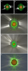 |
Fig. 1. Showcase of visualization of field lines (uniformly sampled) from the model, overplotted to observational white-light data from (a) STEREO B COR1, (b) STEREO A COR1, (c) SOHO LASCO C2, (d) STEREO A COR2, and (e) eclipse picture. The PFSS model is plotted as 3D field line configuration in green, while the SCS solution is plotted in a 2D plane-of-sky slice in yellow. In (a) and (b), Rss = 2.4 R⊙ for 1 Aug. 2008, while in (c), (d), and (e), Rss = 2.9 R⊙ and Rscs = 2.5 R⊙ for 11 Jul. 2010. |
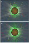 |
Fig. 2. Illustration of visual classification process for two configurations on 11 Jul. 2010 overlaid on eclipse data. Yellow arrows mark good matches between observation and field line simulation, while red arrows mark mismatches. Panel a: thus shows a well-matching configuration (Rss = 1.9 R⊙ and Rscs = 1.5 R⊙), while the field line solution in (b) is rejected by our criteria (Rss = 2.8 R⊙ and Rscs = 2.4 R⊙). |
3.2. Method II: Feature matching
In comparison to the visual inspection described in Method I, a semi-automatized identification of matching white-light features to modeled ones provides a more objective, but more time-consuming (in terms of human intervention), method that results in a quantitative assessment of the quality of model results. To compare different features between model and observational data in an efficient way, we used simple point-and-click algorithms. As there are many possibilities, in Sect. 3.2.1 we compare streamer orientation angles with the SCS field line directions as well as opening angles (width) of streamers with the boundary of closed to open topology in the PFSS. In Sect. 3.2.2, we compare the brute force feature matching to identify differences in the location of certain structures (see Fig. 3).
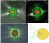 |
Fig. 3. Chosen features and visualization of feature-matching methods with (a) the streamer direction method from II.a (using LASCO C2 for 11 Jul. 2010, Rss = 2.9 R⊙ and Rscs = 1.9 R⊙), (b) the streamer width method from II.a (STEREO A COR1 for 1 Aug. 2008, Rss = 3.0 R⊙), and (c) the brute force matching method from II.b (using an high-resolution eclipse image by Druckmüller for 11 Jul. 2010, Rss = 2.4 R⊙ and Rscs = 1.4 R⊙). In (a), (b), and (c), blue markings result from the observation, while red markings result from the modeled field lines. (d) gives an illustration of the two possible definitions of the streamer width by the underlying closed topology of the model (closed field, angle marked by solid lines; first open field, angle marked by dashed lines). |
3.2.1. Method II.a: Streamer direction and width
Coronal streamers are quasi-static features that are shaped by the global magnetic field structure of the Sun and appear as bright structures in coronagraphs; they are thus well observed without intensive processing of image data. Hence, they are well suited for a comparison with models showing the global coronal magnetic field. Helmet streamers are located above regions of closed field lines, such as active regions or filament channels, with a certain extension (width) and thinning out into a ray-like structure and a radial orientation enveloping a current sheet (see e.g., the review by Koutchmy & Livshits 1992). Similar in appearance but without a current sheet are unipolar pseudo-streamers, connecting two coronal holes of the same polarity (see Wang et al. 2007).
For the streamer direction, we used the SCS model results. These are visualized in 2D slices from which we derive the orientation of field lines in an image plane. We assume that the brightest streamer is lying closer to the image plane; hence, it is ideal for comparing the modeled field in the outer corona to coronagraph images from SOHO/LASCO-C2 and COR2 aboard STEREO-A and -B. We measured the angular difference between the modeled field line and observed streamer orientation over the heights H1 = 3.5 R⊙ to H2 = 6.0 R⊙. The values were chosen such that the model field lines and streamer structure are approximately radial but still well visible in the coronagraph FoV. Panel a of Fig. 3 shows that the directions of both the tracked streamer edge (blue) and the marked field line (red) match quite nicely for this configuration, with the angular difference being only 0.5 degrees, which is well within the uncertainties of the method (see discussion in Sect. 4).
The width of the streamer base structure is observed in the low corona and can be detected from COR1 STEREO-A and -B white-light data over 1.5–4 R⊙. That distance range can be applied to validate modeled coronal magnetic field structures in the PFSS domain of the model. At a fixed height above the photosphere, which was chosen to be H = 1.75 R⊙, we measured the streamer width in the image data and the loop extensions in the model results. An example can be seen in Fig. 3, panel b. Here, the extension of the modeled loop structures surpasses the width of the white-light feature at H = 1.75 R⊙ substantially, with 48.9 degrees for closed fields as the boundary, and 55.3 degrees for open fields as the boundary compared to 34.8 degrees from the white-light image. It thus shows a poorly matching configuration for this sub-step. The height is chosen so that it is well above the occulting disk of the coronagraph in order to avoid stray light effects, but we also required it to be as low as possible in order to capture the loop extension for a maximum of model configurations, especially for those with a low source surface height.
3.2.2. Method II.b: Brute force feature matching
In comparison to coronagraph data, contrast-enhanced solar eclipse images cover the coronal fine structures better due to the Moon being an almost ideal occulter. That enables us to investigate features over large distance ranges with high accuracy. Subsequently, this can be used for a more detailed comparison using feature-matching methods such as brute force, where the positions of features that are suspected to be the same are compared directly via point-and-click. In principle, this provides a large variety of possibilities and is therefore a rather flexible approach of comparing certain features of a model. In panel c of Fig. 3, we compare the apex location of loop systems with that method, as it can be identified well from observational data and from model results. The method has no fixed heights and selects the best observed features.
3.3. Method III: Topology classification
To quantify the quality of the model results in a fully automatized and objective way, we investigated the magnetic field topology. We assumed that the majority of the open field emanates from coronal holes, which are usually observed in EUV as structures of reduced emission (Cranmer 2009) due to reduced density and temperature in contrast with the surrounding quiet Sun (e.g., Heinemann et al. 2021). As the coronal model covers the Sun over 360 degrees, we used synoptic EUV maps for the extraction. Checking the bimodal logarithmic intensity distribution and visually identified boundaries of coronal holes (e.g., Krista & Gallagher 2009; Rotter et al. 2012), we used log(EITdata) = 2.95 as the threshold for 1 Aug. 2008, and log(AIAdata) = 3.5 for 11 Jul. 2010. The extracted coronal hole areas were compared to the computed open field regions from the coronal model. The areas outside coronal holes are assumed to be closed field, and we also compared them with those from the model results. The modeled maps of magnetically open and closed regions were compared with the EUV maps, scaled to the size of each other, by applying three different metrics:
1) the coverage parameter:
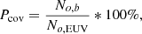
where No, b is the number of pixels that are found to be open in both maps (EUV and model), and No, EUV is the number of open pixels in the EUV map;
2) the Jaccard metric for open fields:
with No, all representing all pixels that are open in either EUV or the model, and
3) the global matching parameter,
with Nmatch the number of pixels where the topology, either open or closed, matches in both maps and Ntot the total number of pixels. To avoid misinterpretation due to the large uncertainties coming from the polar regions, we cut the maps to heliographic latitudes in [−60, +60] degrees and only counted pixels within that range. Pcov was already used to quantify EUHFORIA’s accuracy in modeling coronal hole areas in Asvestari et al. (2019), and it gives the fraction of overlap between modeled and observed open regions. PJac also expresses where model results produce open magnetic field topology not observed in EUV, and Pglob defines the overall correctly modeled topology fraction.
4. Results
The stand-alone methods described in Sect. 3 are most efficient when combined in the frame of a certain workflow. On the basis of EUHFORIA’s coronal model for the two selected dates, 1 Aug. 2008 and 11 Jul. 2010, we present, in the following, a developed sequence of empirical classification and physical and mathematical methods for quantifying and validating the coronal model results. That workflow is depicted in Fig. 4, and below we describe the application from top to bottom. The full set of model parameters covering a total of 67 different configurations as well as the selected subsets (A, B, C) are given in the Appendix in Table A.1.
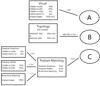 |
Fig. 4. Workflow of our application of the benchmarking system to the EUHFORIA coronal model. In each box on the right, we show comparative images – except in the feature-matching box, where we show the results of each sub-step on the right. Configurations that passed the analysis given in the boxes are sorted into sets A, B, and C. |
We first carried out the visual inspection of off-limb structures (see Sect. 3.1) starting from the full set of 67 model configurations. Observational data were obtained from five different sources: STEREO-A COR1, STEREO-B COR1, STEREO-A COR2, LASCO-C2 and eclipse images. We note that STEREO-B COR2 images only show low-intensity structures for both dates and were therefore not used for further analysis. We then visually inspected these images and checked the general match with the observations for PFSS in the lower corona and the field line bending as derived from the SCS model. We find, on one hand, that the larger values of SCS boundary height produce field line bendings at distances where streamers are observed to be already mostly radial. On the other hand, the low end of the Rscs parameter value spectrum shows a strictly radial behavior of field lines where bending can still be seen in observational data. Hence, we may restrict our parameter set so that heights in the lower to mid value range of the parameter spectrum of the SCS model are preferred. For both dates, 1 Aug. 2008 and 11 Jul. 2010, the best visual match is found in the Rscs ∈ [1.5; 2.1] R⊙ interval. If three out of five images showed a good visual match with the model results from the different perspectives, we kept that model configuration and formed selection set A (cf., Fig. 4), consisting of 30/32 parameter sets for 1 Aug. 2008/11 Jul. 2010.
Using the full set of model parameters, we applied, in the next step of our workflow, the topology classification for determining the match between open and closed magnetic field on the Sun, and we calculated the three parameters Pcov, PJac, and Pglob (see Sect. 3.3). Figures 5 and 6 show the EUV Carrington maps for 1 Aug. 2008 (Carrington rotation number 2072) and 11 Jul. 2010 (Carrington rotation number 2098), respectively. The extracted coronal hole areas are overplotted together with the computed contours of EUHFORIA’s open magnetic field. As can be seen for both dates, when changing the boundary heights for Rss and Rscs, the computed open field area varies strongly, and the lower these heights are, the more open field regions are generated. This is expected since lowering the Rss height allows for more field lines to be considered as open by the model. The quantification of the overlap between modeled and observed open and closed field is given by the topology parameters described in the previous section.
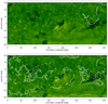 |
Fig. 5. EIT EUV Carrington map for 1 Aug. 2008 with the extracted open areas outlined in black. Open fields were computed with EUHFORIA (white outlines) for the configuration of Rss = 3.2 R⊙ and Rscs = 2.8 R⊙ (top) as well as the configuration of Rss = 1.4 R⊙ and Rscs = 1.3 R⊙ (bottom). |
Figures 7 and 8 present the results from the different topology parameters together with the results from the visual classification. For both dates, we find that a lot of the highest scoring configurations from the topology analysis also passed the visual classification (indicated by large dots). For 1 Aug. 2008, the three topology parameters behave differently, highlighting the different properties that the metrics measure. Results for PJac reveal an increase in match with increasing Rss, and consequently also with increasing Rscs, up to a turning point at about 2.5 R⊙. The parameter Pcov follows the expected trend of a continuous decrease with increasing configuration parameter values. This is due to the fact that with increasing Rss and increasing Rscs, less and less open field is generated by the model. Hence, the percentage of overlap of the model and observed open fields decreases. Inversely to Pcov, the global parameter Pglob increases with increasing Rss and Rscs.
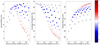 |
Fig. 7. Behavior of PJac, Pcov, and Pglob with varying PFSS and SCS heights for 1 Aug. 2008. The color bar indicates the SCS heights, crosses mark configurations that failed in the visual classification, while dots mark configurations that passed it. |
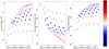 |
Fig. 8. Behavior of PJac, Pcov, and Pglob with varying PFSS and SCS heights for 11 Jul. 2010. The color bar indicates the SCS heights, crosses mark configurations that failed in the visual classification, while dots mark configurations that passed it. |
For 11 Jul. 2010, the results are slightly different as Pglob and PJac follow very similar trends; namely, they increase if either Rss or Rscs increases, with the latter having the bigger impact. This means that there is a clear trend in which modeling less open structures matches better with the EUV observations for that date. Rscs is the dominating parameter here and could be used as a limiting factor of open structures. This is because while the PFSS sets the magnetic topology, Rscs serves as the cut-off for the PFSS-domain and thus decides how much of the magnetic field is actually open. The model configuration that produces the lowest amount of open fields, which is the one with the highest Rss and Rscs values, covers 3.88% of the total area in comparison to the EUV observations giving about 3.00%. The overestimation of open areas from the model for that date is also the reason for the inverse behavior of Pcov with respect to Pglob and PJac, as Pcov is insensitive to overestimation and solely measures overlap regions between the model and EUV. Hence, PJac should be used complementarily to Pcov in order to derive the amount of overestimation of modeled open magnetic field areas.
The most general parameter we introduced here is Pglob, which gives the fraction of matching pixels in the masks over the total number of pixels of the entire map. Therefore, Pglob best reflects the quality of the modeled output and is used as a criterion for rejecting parameter sets of lower quality. We reduced the set of configurations by using the best 50% from the distribution given by Pglob, and subsequently, we formed set B (cf. Fig. 4). Set B consists, as per the definition of our criteria, of 33 parameter sets for both dates. We note that PJac would give similar results, especially for the 11 Jul. 2010 event. Interestingly, while there is a significant match between both the visual inspection step and the topology analysis, we can see in Figs. 7 and 8 that the visual inspection would actually reject not only the worst configurations from the topology analysis, but also the best matching ones. We note that while for some configurations the general topology matches well, this does not necessarily mean that the field line trajectories also match when compared to white-light images. This implies that analyzing modeled open and closed fields yields additional information that cannot be derived through mere comparison of the field line configuration with white-light data and vice versa.
Starting again from the full set of model parameters, in the last step of the workflow we applied the feature-matching method (see Sect. 3.2). Using a semi-automatized algorithm, we manually selected the brightest features (assuming that those lie closest to the plane of sky) from the white-light data and compared that with the modeled field lines (point-and-click method). Streamers can be characterized by their direction and width in the lower corona. Figure 9 shows the differences in the angles derived between modeled field line and observed streamer direction for both dates in relation to the chosen SCS heights, and the PFSS heights are given by multiple dots for the same Rscs. Error bars reveal average uncertainties in the plane-of-sky selection for the SCS model results as these are 2D visualization slices. To define the error bars, we simply varied the longitudinal direction by +/−10 degrees. We also investigated point-and-click inaccuracies but yielded a very minor effect compared to the errors as derived by the tilting procedure. For almost all chosen structures that we investigated, an approximately linear trend across the SCS height spectrum is obtained. The choice of the PFSS model boundary height seems to have a negligible influence on the resulting SCS field lines. One exception is the chosen feature from the LASCO perspective for 1 Aug. 2008, where no significant variation in the field line angle could be measured by using different model parameter sets. As can be seen in Fig. 9, for all the streamer directions there is no clear ideal SCS parameter derivable, most likely due to large errors originating from the uncertainty in the longitudinal streamer location itself.
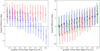 |
Fig. 9. Difference between SCS field line angle and streamer angle from observations for 1 Aug. 2008 (left) and 11 Jul. 2010 (right). Red marks the results from SOHO/LASCO perspective, while blue and green are the results for STEREO/COR2. Multiple dots for a fixed SCS height indicate the different PFSS heights for the same Rscs. |
A more decisive picture is created by comparing the streamer width with the angular extension of underlying loop systems in the PFSS model. We derived the streamer widths from the white-light data as 34.8 and 18.6 degrees for the features selected for 1 Aug. 2008 and 16.9 and 35.0 degrees for 11 Jul. 2010 for Stereo A and B, respectively. The results are given in Fig. 10 and we obtain that configurations with [Rss ∈ 2.0 R⊙; 2.5 R⊙] seem to perform best for both dates. The errors originate from both the visualization bias, due to manually selecting which field lines are chosen to display, and the uncertainty due to the definition of the streamer width, either marking the closed loop system or the closest open field lines next to that closed system, as shown in Fig. 3d). After extensive testing, we conclude that the point-and-click errors are comparatively small next to these error sources.
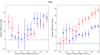 |
Fig. 10. Difference of PFSS closed structure width and streamer width from observations for both 1 Aug. 2008 (left) and 11 Jul. 2010 (right). Red marks results originating from STEREO A, while the STEREO B results are shown in blue. |
The final routine we implemented involves brute force feature matching to compare the location of prominent features such as the top of closed-loop systems from PFSS results. As this requires a rather accurate identification of white-light structures for the comparison, high-resolution solar eclipse photographs are used for this analysis. Figure 11 shows the results with error bars coming from the visualization bias that the model results are imposed upon by the selection of a set of field lines. The lowest differences between model and observations are derived for configurations with Rss ∈ [2.0, 2.5] R⊙. Based on that we obtain a similar outcome as for the streamer width analysis (see Fig. 10).
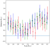 |
Fig. 11. 2D-projected positional difference of PFSS loop structures and loop systems from eclipse observations by Druckmüller for both 08-01-2008 (crosses) and 07-11-2010 (triangles). Different colors indicate different features. |
Results from the feature matching method form set C in our workflow. Set C covers configurations for which, for at least two out of three matched features, the error bars reach the line of zero difference in relation to the observations, namely, the blue horizontal lines in Figs. 9, 10, and 11. It consists of 11 parameter sets for both dates.
Inspecting the overlap in the reduced sets from A, B, and C (Table A.1), we combined the quality assessment of visual, topology, and feature-matching classifications. Interestingly, there is one configuration that passed all three sub-steps for both dates. This configuration is Rscs = 2.0 R⊙, Rss = 2.4 R⊙, and it marks our derived ideal parameter set for this exemplary analysis.
5. Discussion
In this study, we developed a validation scheme that acts as a guideline for a standardized quality assessment of coronal model results. It presents a tool for modelers that can be easily applied in order to chose the most reliable option(s) of model input data and parameters among the many different possible ones. With the example of the EUHFORIA coronal model, we define classification steps based on comparing PFSS and SCS model results with observational data from different perspectives. The classification steps cover a visual comparison of global open and closed magnetic field structures and isolated features, as well as mathematical metrics, and they can be used in an objective way to reduce the initial set of model configurations down to the most reliable ones.
To separate the initial set into good or bad matching model configurations, we used a visual inspection focusing on the magnetic field line bending in the SCS model, close to the lower boundary, and compared that to coronagraph data from different instruments. We find that the visual comparison is subjective, but it can be performed rather easily and may quickly sort out a large set of parameter values. It is also a useful tool for investigating properties, such as the SCS bending, that cannot easily be determined by either the topology parameters or the feature-matching classification.
An objective classification is given by the topology analysis, which uses the information of open magnetic field on the Sun as extracted from synoptic EUV image data. Via an intensity threshold, we performed a simple detection of dark areas in the EUV data that presumably represent coronal holes, which are the dominant source of open magnetic field and fast solar wind from the Sun (for a review see e.g., Cranmer & Winebarger 2019). We applied different parameters to compare the model results with the observations such as Pcov (to assess the performance of a model configuration with focus on open field computation, but ignoring areas outside of EUV-open regions; see Asvestari et al. 2019), PJac (to assess the amount under and overestimating the open field computation, giving the percentage of similarity between the model- and EUV-open regions), and Pglob (to assess the overall performance of specific model configurations, as it is the plain overlap percentage of both masks including closed regions). We find that Pcov and PJac values for 1 Aug. 2008 are much lower compared to those from 11 Jul. 2010 and the comparison is left to the Pglob parameter. We find that model configurations revealing a low percentage in the topology parameters were also rejected from the visual inspection. The boundary height of Rscs dominates the computed amount of open field, and in general heights above ∼2 R⊙ yield a better match to the observations. Uncertainties for that method definitely come from the assumption that open magnetic field predominantly originates from dark structures, as observed in EUV and by using synoptic EUV data, representing the coronal structures over a full solar rotation (the same holds for the magnetic field input used for the model). The uncertainties in the dark area (i.e., coronal hole) extraction itself are found to lie in the range of ±25% (Linker et al. 2021). Taking that into account, the coronal model is still at the lower limit of matching with observations and generally overestimates the open magnetic field areas. In a recent paper by Asvestari et al. (2019), it was shown that this has a negligible effect when using more coarse model resolutions of about 2 degrees per pixel. Moreover, EIT images (1 Aug. 2008) seem to be more noisy compared to the AIA image data (11 Jul. 2010), and the two dates under study cover different phases in the solar activity cycle, with 2010 being a more active time compared to the minimum phase during 2008. High activity might cause large deviations from a steady-state condition and strong changes for the synoptic data used (as input and for the comparison). Nevertheless, the 2010 date produces better numerical results in the topology analysis.
For the first feature matching method, we obtain a strong dominance of Rscs for most of the results. Thus, the field line appearance of the SCS model only weakly depends on varying the source surface parameter Rss of the underlying PFSS model. While the streamer angle comparison is found to be only a weak filter (a big portion of configurations pass with 33 of 67 for 1 Aug. 2008 and 61 out of 67 for 11 Jul. 2010), the situation is very different when comparing the width of the streamer and the brute force matching method. Applying those classifications, we obtain an overall combined number of only 11 configurations left in set C for each date.
Our final conclusion regarding our creation of a benchmarking system for EUHFORIA is that the coronal model configuration with Rscs = 2.0 R⊙, Rss = 2.4 R⊙ is the ideal parameter set for the analyzed dates. While a more in-depth analysis with a broader selection of dates would be necessary to draw a more comprehensive conclusion, this result matches within the expected range in parameter space and conforms with current defaults and conventions (see e.g., Mackay & Yeates 2012; Pomoell & Poedts 2018).
The possible sequence of the classification steps as described do not depend on each other and can be applied in any desired order. For a large number of model configurations under investigation, we may suggest combining methods A and B to reduce the parameter sets before further analysis. The strength of combining these two methods lies in the combination of empirical visual classification with a mathematical scheme.
Input data and parameters for any coronal model underlie large variations and generate plentiful results that need to be assessed in terms of quality and reliability with respect to observations. Standardized validation schemes, as presented here, are a necessity for model improvement leading to more reliable space weather forecasts (see also MacNeice et al. 2018; Hinterreiter et al. 2019; Verbeke et al. 2019). Moreover, more reliable model results provide a basis for better understanding the interplay between global open and closed magnetic field configuration resulting in the different solar wind structures, which in turn leads to a better understanding of the propagation characteristics of coronal mass ejections in interplanetary space.
Acknowledgments
A.W. acknowledges financial support by the CCSOM project. E.A. acknowledges the support of the Academy of Finland (Project TRAMSEP, Academy of Finland Grant 322455).
References
- Arge, C. N., & Pizzo, V. J. 2000, J. Geophys. Res., 105, 10465 [Google Scholar]
- Asvestari, E., Heinemann, S. G., Temmer, M., et al. 2019, J. Geophys. Res. (Space Phys.), 124, 8280 [NASA ADS] [CrossRef] [Google Scholar]
- Brueckner, G. E., Howard, R. A., Koomen, M. J., et al. 1995, Sol. Phys., 162, 357 [NASA ADS] [CrossRef] [Google Scholar]
- Case, A. W., Spence, H. E., Owens, M. J., Riley, P., & Odstrcil, D. 2008, Geophys. Res. Lett., 35, L15105 [NASA ADS] [CrossRef] [Google Scholar]
- Childs, H., Brugger, E., Whitlock, B., et al. 2012, High Performance Visualization-Enabling Extreme-Scale Scientific Insight, 357 [Google Scholar]
- Cohen, O., Sokolov, I. V., Roussev, I. I., & Gombosi, T. I. 2007, AGU Fall Meeting Abstracts, 2007, SH51B-06 [NASA ADS] [Google Scholar]
- Couvidat, S., Schou, J., Hoeksema, J. T., et al. 2016, Sol. Phys., 291, 1887 [Google Scholar]
- Cranmer, S. R. 2009, Liv. Rev. Sol. Phys., 6, 3 [Google Scholar]
- Cranmer, S. R., & Winebarger, A. R. 2019, ARA&A, 57, 157 [Google Scholar]
- Cranmer, S. R., Gibson, S. E., & Riley, P. 2017, Space Sci. Rev., 212, 1345 [Google Scholar]
- Domingo, V., Fleck, B., & Poland, A. I. 1995, Sol. Phys., 162, 1 [Google Scholar]
- Druckmüller, M. 2009, ApJ, 706, 1605 [CrossRef] [Google Scholar]
- Druckmüller, M., Rušin, V., & Minarovjech, M. 2006, Contrib. Astron. Obs. Skaln. Pleso, 36, 131 [Google Scholar]
- Harvey, J. W., Hill, F., Hubbard, R. P., et al. 1996, Science, 272, 1284 [Google Scholar]
- Heinemann, S. G., Saqri, J., Veronig, A. M., Hofmeister, S. J., & Temmer, M. 2021, Sol. Phys., 296, 18 [NASA ADS] [CrossRef] [Google Scholar]
- Hess Webber, S. A., Karna, N., Pesnell, W. D., & Kirk, M. S. 2014, Sol. Phys., 289, 4047 [NASA ADS] [CrossRef] [Google Scholar]
- Hinterreiter, J., Magdalenic, J., Temmer, M., et al. 2019, Sol. Phys., 294, 170 [NASA ADS] [CrossRef] [Google Scholar]
- Howard, R. A., Moses, J. D., Socker, D. G., et al. 2002, Adv. Space Res., 29, 2017 [NASA ADS] [CrossRef] [Google Scholar]
- Howard, R. A., Moses, J. D., Vourlidas, A., et al. 2008, Space Sci. Rev., 136, 67 [NASA ADS] [CrossRef] [Google Scholar]
- Jian, L. K., MacNeice, P. J., Mays, M. L., et al. 2016, Space Weather, 14, 592 [CrossRef] [Google Scholar]
- Kaiser, M. L. 2005, Adv. Space Res., 36, 1483 [NASA ADS] [CrossRef] [Google Scholar]
- Kaiser, M. L., Kucera, T. A., Davila, J. M., et al. 2008, Space Sci. Rev., 136, 5 [Google Scholar]
- Karna, N., Hess Webber, S. A., & Pesnell, W. D. 2014, Sol. Phys., 289, 3381 [NASA ADS] [CrossRef] [Google Scholar]
- Koutchmy, S., & Livshits, M. 1992, Space Sci. Rev., 61, 393 [CrossRef] [Google Scholar]
- Krista, L. D., & Gallagher, P. T. 2009, Sol. Phys., 256, 87 [Google Scholar]
- Linker, J. A., Heinemann, S. G., Temmer, M., et al. 2021, ApJ, 918, 21 [CrossRef] [Google Scholar]
- Mackay, D. H., & Yeates, A. R. 2012, Liv. Rev. Sol. Phys., 9, 6 [Google Scholar]
- MacNeice, P., Jian, L. K., Antiochos, S. K., et al. 2018, Space Weather, 16, 1644 [NASA ADS] [CrossRef] [Google Scholar]
- McGregor, S. L., Hughes, W. J., Arge, C. N., & Owens, M. J. 2008, J. Geophys. Res. (Space Phys.), 113, A08112 [Google Scholar]
- Meyer, K. A., Mackay, D. H., Talpeanu, D.-C., Upton, L. A., & West, M. J. 2020, Sol. Phys., 295, 101 [NASA ADS] [CrossRef] [Google Scholar]
- Morgan, H., Habbal, S. R., & Woo, R. 2006, Sol. Phys., 236, 263 [Google Scholar]
- Pesnell, W. D., Thompson, B. J., & Chamberlin, P. C. 2012, Sol. Phys., 275, 3 [Google Scholar]
- Pomoell, J., & Poedts, S. 2018, J. Space Weather Space Clim., 8, A35 [NASA ADS] [CrossRef] [EDP Sciences] [Google Scholar]
- Riley, P., Ben-Nun, M., Linker, J. A., et al. 2014, Sol. Phys., 289, 769 [Google Scholar]
- Riley, P., Mays, M. L., Andries, J., et al. 2018, Space Weather, 16, 1245 [NASA ADS] [CrossRef] [Google Scholar]
- Rotter, T., Veronig, A. M., Temmer, M., & Vršnak, B. 2012, Sol. Phys., 281, 793 [CrossRef] [Google Scholar]
- Sachdeva, N., Subramanian, P., Colaninno, R., & Vourlidas, A. 2015, ApJ, 809, 158 [NASA ADS] [CrossRef] [Google Scholar]
- Sasso, C., Pinto, R. F., Andretta, V., et al. 2019, A&A, 627, A9 [NASA ADS] [CrossRef] [EDP Sciences] [Google Scholar]
- Schatten, K. H. 1971, Cosm. Electrodyn., 2, 232 [NASA ADS] [Google Scholar]
- Schmidt, J. M., & Cargill, P. J. 2001, J. Geophys. Res., 106, 8283 [NASA ADS] [CrossRef] [Google Scholar]
- Schou, J., Scherrer, P. H., Bush, R. I., et al. 2012, Sol. Phys., 275, 229 [Google Scholar]
- Sheeley, N. R., Wang, Y. M., Hawley, S. H., et al. 1997, ApJ, 484, 472 [Google Scholar]
- Temmer, M. 2021, Liv. Rev. Sol. Phys., 18, 4 [NASA ADS] [CrossRef] [Google Scholar]
- Temmer, M., Rollett, T., Möstl, C., et al. 2011, ApJ, 743, 101 [NASA ADS] [CrossRef] [Google Scholar]
- Verbeke, C., Mays, M. L., Temmer, M., et al. 2019, Space Weather, 17, 6 [CrossRef] [Google Scholar]
- Vršnak, B. 2021, J. Space Weather Space Clim., 11, 34 [CrossRef] [EDP Sciences] [Google Scholar]
- Wang, Y. M., Sheeley, N. R. J., & Rich, N. B. 2007, ApJ, 658, 1340 [CrossRef] [Google Scholar]
- Yeates, A. R., Amari, T., Contopoulos, I., et al. 2018, Space Sci. Rev., 214, 99 [CrossRef] [Google Scholar]
Appendix A: Full list of model parameter sets
Table A.1 lists the full set of model parameters that were used to produce 67 different configurations in the EUHFORIA coronal model results as used for the analysis given in Section 4. In addition, for each date (2008 and 2010), we give the parameter sets that passed (x) the criteria for visual (A), topology (B), or feature matching (C) classification.
Parameter sets used with the PFSS and SCS model heights for the analysis as described in Section 4. Those parameter sets that passed the criteria for high quality in the visual (A), topology (B), or feature-matching (C) classification scheme are marked by x.
All Tables
Parameter sets used with the PFSS and SCS model heights for the analysis as described in Section 4. Those parameter sets that passed the criteria for high quality in the visual (A), topology (B), or feature-matching (C) classification scheme are marked by x.
All Figures
|
Fig. 1. Showcase of visualization of field lines (uniformly sampled) from the model, overplotted to observational white-light data from (a) STEREO B COR1, (b) STEREO A COR1, (c) SOHO LASCO C2, (d) STEREO A COR2, and (e) eclipse picture. The PFSS model is plotted as 3D field line configuration in green, while the SCS solution is plotted in a 2D plane-of-sky slice in yellow. In (a) and (b), Rss = 2.4 R⊙ for 1 Aug. 2008, while in (c), (d), and (e), Rss = 2.9 R⊙ and Rscs = 2.5 R⊙ for 11 Jul. 2010. |
| In the text | |
|
Fig. 2. Illustration of visual classification process for two configurations on 11 Jul. 2010 overlaid on eclipse data. Yellow arrows mark good matches between observation and field line simulation, while red arrows mark mismatches. Panel a: thus shows a well-matching configuration (Rss = 1.9 R⊙ and Rscs = 1.5 R⊙), while the field line solution in (b) is rejected by our criteria (Rss = 2.8 R⊙ and Rscs = 2.4 R⊙). |
| In the text | |
|
Fig. 3. Chosen features and visualization of feature-matching methods with (a) the streamer direction method from II.a (using LASCO C2 for 11 Jul. 2010, Rss = 2.9 R⊙ and Rscs = 1.9 R⊙), (b) the streamer width method from II.a (STEREO A COR1 for 1 Aug. 2008, Rss = 3.0 R⊙), and (c) the brute force matching method from II.b (using an high-resolution eclipse image by Druckmüller for 11 Jul. 2010, Rss = 2.4 R⊙ and Rscs = 1.4 R⊙). In (a), (b), and (c), blue markings result from the observation, while red markings result from the modeled field lines. (d) gives an illustration of the two possible definitions of the streamer width by the underlying closed topology of the model (closed field, angle marked by solid lines; first open field, angle marked by dashed lines). |
| In the text | |
|
Fig. 4. Workflow of our application of the benchmarking system to the EUHFORIA coronal model. In each box on the right, we show comparative images – except in the feature-matching box, where we show the results of each sub-step on the right. Configurations that passed the analysis given in the boxes are sorted into sets A, B, and C. |
| In the text | |
|
Fig. 5. EIT EUV Carrington map for 1 Aug. 2008 with the extracted open areas outlined in black. Open fields were computed with EUHFORIA (white outlines) for the configuration of Rss = 3.2 R⊙ and Rscs = 2.8 R⊙ (top) as well as the configuration of Rss = 1.4 R⊙ and Rscs = 1.3 R⊙ (bottom). |
| In the text | |
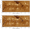 |
Fig. 6. Same as Fig. 5, but for the AIA EUV Carrington map for 11 Jul. 2010. |
| In the text | |
|
Fig. 7. Behavior of PJac, Pcov, and Pglob with varying PFSS and SCS heights for 1 Aug. 2008. The color bar indicates the SCS heights, crosses mark configurations that failed in the visual classification, while dots mark configurations that passed it. |
| In the text | |
|
Fig. 8. Behavior of PJac, Pcov, and Pglob with varying PFSS and SCS heights for 11 Jul. 2010. The color bar indicates the SCS heights, crosses mark configurations that failed in the visual classification, while dots mark configurations that passed it. |
| In the text | |
|
Fig. 9. Difference between SCS field line angle and streamer angle from observations for 1 Aug. 2008 (left) and 11 Jul. 2010 (right). Red marks the results from SOHO/LASCO perspective, while blue and green are the results for STEREO/COR2. Multiple dots for a fixed SCS height indicate the different PFSS heights for the same Rscs. |
| In the text | |
|
Fig. 10. Difference of PFSS closed structure width and streamer width from observations for both 1 Aug. 2008 (left) and 11 Jul. 2010 (right). Red marks results originating from STEREO A, while the STEREO B results are shown in blue. |
| In the text | |
|
Fig. 11. 2D-projected positional difference of PFSS loop structures and loop systems from eclipse observations by Druckmüller for both 08-01-2008 (crosses) and 07-11-2010 (triangles). Different colors indicate different features. |
| In the text | |
Current usage metrics show cumulative count of Article Views (full-text article views including HTML views, PDF and ePub downloads, according to the available data) and Abstracts Views on Vision4Press platform.
Data correspond to usage on the plateform after 2015. The current usage metrics is available 48-96 hours after online publication and is updated daily on week days.
Initial download of the metrics may take a while.