| Issue |
A&A
Volume 657, January 2022
|
|
|---|---|---|
| Article Number | A48 | |
| Number of page(s) | 6 | |
| Section | Stellar structure and evolution | |
| DOI | https://doi.org/10.1051/0004-6361/202038582 | |
| Published online | 04 January 2022 | |
Constraints on the orbital separation distribution and binary fraction of M dwarfs
Department of Astronomy, University of Michigan, Ann Arbor, MI, USA
e-mail: nsusemiehl@gmail.com
Received:
4
June
2020
Accepted:
9
September
2021
Aims. We present a new estimate for the binary fraction (the fraction of stars with a single companion) for M dwarfs using a log-normal fit to the orbital separation distribution.
Methods. We used point estimates of the binary fraction (binary fractions over specific separation and companion mass ratio ranges) from four M dwarf surveys sampling distinct orbital radii to fit a log-normal function to the orbital separation distribution. This model, alongside the companion mass ratio distribution given by Reggiani & Meyer (2013, A&A, 553, A124), is used to calculate the frequency of companions over the ranges of mass ratio (q) and orbital separation (a) over which the referenced surveys were collectively sensitive – [0.60 ≤ q ≤ 1.00] and [0.00 ≤ a ≤ 10 000 AU]. This method was then extrapolated to calculate a binary fraction which encompasses the broader ranges of [0.10 ≤ q ≤ 1.00] and [0.00 ≤ a < ∞ AU]. Finally, the results of these calculations were compared to the binary fractions of other spectral types.
Results. The binary fraction over the constrained regions of [0.60 ≤ q ≤ 1.00] and [0.00 ≤ a ≤ 10 000 AU] was calculated to be 0.229 ± 0.028. This quantity was then extrapolated over the broader ranges of q (0.10−1.00) and a (0.00 − ∞ AU) and found to be 0.462−0.052+0.057. We used a conversion factor to estimate the multiplicity fraction from the binary fraction and found the multiplicity fraction over the narrow region of [0.60 ≤ q ≤ 1.00] and [0.00 ≤ a ≤ 10 000 AU] to be 0.270 ± 0.111. Lastly, we estimated the multiplicity fractions of FGK, and A stars using the same method (taken over [0.60 ≤ q ≤ 1.00] and [0.00 ≤ a ≤ 10 000 AU]). We find that the multiplicity fractions of M, FGK, and A stars, when considered over common ranges of q and a, are more similar than generally assumed.
Key words: binaries: general / stars: late-type / stars: statistics
© N. Susemiehl and M. R. Meyer 2022
 Open Access article, published by EDP Sciences, under the terms of the Creative Commons Attribution License (http://creativecommons.org/licenses/by/4.0), which permits unrestricted use, distribution, and reproduction in any medium, provided the original work is properly cited.
1. Introduction
Because M dwarfs comprise as much as 75% of local stellar populations (Henry et al. 2006; Winters et al. 2019, and references therein), it is important to have an accurate census of their properties. Understanding the multiplicity fraction, that is, the fraction of stellar systems with one or more gravitationally-bound companion (regardless of whether it is above or below the hydrogen burning limit), of M dwarfs will have significant implications for star formation theories, providing information about the emergence of planetary systems around low mass stars and allowing for the modeling of both galactic and extra-galactic stellar populations. A related quantity is the binary fraction, the fraction of stars with a single gravitationally bound companions. The key difference between these two statistics is that the multiplicity fraction considers systems with more than two companions while the binary fraction does not. Mathematically, these quantities are expressed as  and
and  (where MF denotes the multiplicity fraction, BF the binary fraction, and NS, ND, NT, NH the number of single, double, triple, and higher order systems respectively). These differences extend to formation theories: the multiplicity fraction may be more related to gravitational fragmentation of star forming molecular cloud cores than the more simple binary fraction (cf. Raghavan et al. 2010; De Rosa et al. 2014). In addition, differences between the multiplicity and binary fractions as a function of primary star mass are another key constraint of formation theory. Multiple conventions exist to define the mass ratio and orbital distribution for higher order systems, so we only consider the binary fraction when fitting our model in order to avoid these complications. Despite the importance of this feature, the multiplicity properties of M dwarfs are not yet fully understood.
We modeled the binary fraction using the companion mass ratio distribution (ψ) and orbital separation distribution (ϕ). The companion mass ratio distribution represents the fraction of stars which have a companion within a given range of the mass ratio. The mass ratio, q, is defined as the ratio between the mass of a secondary star and the mass of the respective primary star where, by definition, the mass of the primary star is greater than that of the secondary, so that q ≤ 1. The orbital separation distribution is the fraction of stars which have a companion as a function of the separation between the two stars. The semi-major axis of an orbital ellipse, a, serves as a measure of the separation between the primary and secondary stars. Integrating either of these functions over specific ranges of their respective parameters returns the fraction of M dwarfs which have a single companion over that range if one assumes the other parameter has been integrated over its full parameter space. Thus, ψ and ϕ must be combined to provide a binary fraction over a fixed ranges of q and a, calculated as:
where qmin, qmax, log10amin, and log10amax represent the lower and upper bounds for the mass ratio and semi-major axes of interest.
The companion mass ratio distribution is discussed in Reggiani & Meyer (2013), who find that

which describes this distribution for M dwarfs as well as field FGK stars and intermediate mass stars in the young ScoOB2 association. The present work attempts to fit the functional form ϕ for the orbital separation distribution.
This method for calculating the binary fraction is built upon a key assumption, namely: the companion mass ratio distribution does not depend on the orbital separation. This assumption allows for the calculation of binary fractions using Eq. (1). Reggiani & Meyer (2013) investigated this assumption for M dwarfs based on the data of Janson et al. (2012) and were unable to reject it. Furthermore, we take into consideration only binary systems – and not triplets, quadruplets, etc. We further discuss these caveats in Sect. 4.
Numerous attempts have been made to constrain the multiplicity of M dwarfs (e.g., Fischer & Marcy 1992; Janson et al. 2012; Winters et al. 2019), but none have included samples of stellar binary pairs that are complete over the full ranges of mass ratio (0 ≤ q ≤ 1) or separation (0 < a < ∞). Instead, observational results are necessarily limited to specific ranges of parameters. These past works have set useful constraints on important parameters regarding the population of M dwarfs. For instance, Fischer & Marcy (1992) found that about 42 ± 9% of nearby M dwarfs (with mass ratio 0.2 < q < 1 and separation 0 < a < 10 000 AU) have a companion and Ward-Duong et al. (2015) estimated a companion star fraction of 23.5%±3.2% over a similarly wide region of the parameter space (3 < a < 10 000 AU, 0.2 < q < 1). Janson et al. (2012) suggests that the multiplicity of M dwarfs is intermediate between that of higher-mass stars and brown dwarfs. Cortés-Contreras et al. (2017) found a peak in the orbital separation distribution of M dwarf multiple system at 2.5−7.5 AU, which is similar to the broad peak at around 4−20 AU found by Winters et al. (2019) (cf. Winters et al. 2021). In Sect. 2 of this paper, we describe the methods used to fit the orbital separation distribution and calculate the binary fraction. In Sect. 3, the results are presented. In Sect. 4, we discuss the implications and further investigate the assumptions used. Section 5 summarizes our work.
2. Methods
2.1. Data
The first step in exploring the orbital separation distribution and binary fraction of M dwarfs was to synthesize point estimates of the binary fraction from a variety of different M dwarf surveys. Data was compiled from surveys which employed the radial velocity (Delfosse et al. 1999) and direct imaging (Cortés-Contreras et al. 2017; Janson et al. 2012; Ward-Duong et al. 2015) companion detection methods. This allowed us to investigate companions over a broad range of semi-major axes. The projected separations from the direct imaging surveys of Cortés-Contreras et al. (2017) and Ward-Duong et al. (2015) were converted to physical separations using the correction factor described in Fischer & Marcy (1992) of 1.26 (Janson et al. 2012 already made a correction using this factor). Other works, including Dupuy & Liu (2011), suggest alternative forms to this correction factor that account for other orbital parameters such as eccentricity, but the correction factor estimated by Dupuy & Liu (2011) ( ) is similar to the 1.26 suggested by Fischer & Marcy (1992).
We include only detected multiple systems associated with values of mass ratio and semi-major axis over which each survey was at least 90% complete. The lower limit on mass ratio considered was set by Cortés-Contreras et al. (2017) as q ≥ 0.60. Any detected multiple system which was separated by a distance outside the range that each particular survey was at least 90% complete was also removed (i.e., no longer considered a detection of a binary system). We also excluded any higher order systems by dropping such systems from what we consider to be companions but including them in the total primary star number, effectively treating these systems as single stars. Delfosse et al. (1999) detected six higher order systems, Cortés-Contreras et al. (2017) detected four, Janson et al. (2012) detected 14, and Ward-Duong et al. (2015) detected 5. The binary fraction point estimates for each survey were calculated by dividing the remaining number of binary pairs by the total parent population of each survey. The error bars on the binary fraction point estimates were taken to be the Poisson counting error of the respective surveys (calculated after the aforementioned cleaning steps). Table 1 gives the point estimate of the binary fraction for each survey along with the respective detection method and range of semi-major axis. Similarly, Table 2 depicts the total number of parent stars surveyed and the number of companion detections for each reference.
Binary fraction point estimates, q ≥ 0.6.
Survey details.
In certain cases, assumptions had to be made about details of the surveys. Delfosse et al. (1999) reported the period and orbital velocity of stars in their sample, but not the semi-major axis. Kepler’s Third Law and the masses of the primaries were used to convert the given values into semi-major axes. Janson et al. (2012) did not note the minimum mass ratio that the survey could detect. According to the method in this paper, in every case where qm * ma < 0.08 M⊙, the system is removed from the analysis and only stars with a primary mass > 0.2 M⊙ were included, since, as the authors note, lower-mass stars are not fully complete out to 52 pc (Janson et al. 2012). Based this, we took a minimum secondary mass of 0.08 M⊙ and a minimum primary mass of 0.2 M⊙ to calculate a minimum mass ratio of 0.4. Both Janson et al. (2012) and Ward-Duong et al. (2015) included a small number of multiple systems with K-type primary stars, each of which was removed from this analysis. The data from Ward-Duong et al. (2015) was split into two bins by orbital separation: 0−100 AU and 100−10 000 AU because it covers such a wide range of semi-major axes (3−10 000 AU).
In order to justify our use of the Reggiani & Meyer (2013) power law (Eq. (2)), we employed the Kolmogorov–Smirnov (KS) test to compare the mass ratio samples of Ward-Duong et al. (2015) and Cortés-Contreras et al. (2017) to those drawn from the mass ratio power-law distribution of Reggiani & Meyer (2013) (considering only q > 0.6; Fischer & Marcy 1992; Janson et al. 2012 were used to fit the power law of Reggiani & Meyer 2013 and, thus, were not tested here). These KS tests returned p-values of 0.04 and 0.02, respectively. Based on these p-values, we do not reject the null hypothesis that there is no difference between the distributions of Ward-Duong et al. (2015) and Cortés-Contreras et al. (2017), and the mass ratio distribution proposed by Reggiani & Meyer (2013) at the 0.01 significance level. As an alternative, a future similar work could consider using the mass ratio distribution offered by El-Badry et al. (2019), which suggests a broken power law fit and found an excess of near-equal mass systems. Using this mass ratio distribution would likely change the results found in this study.
2.2. Fitting the model
We fit a log-normal model to the orbital separation distribution of the M dwarf binary systems by using the binary fraction point estimates from the referenced surveys (Table 1) as benchmarks to those computed using Eq. (1). This model (Eq. (3)) has as its free parameters an amplitude (A) that normalizes the function, a mean (μ) that indicates the peak of the distribution, and a standard deviation (σ) that describes the spread of the distribution:
In order to fit the model and find the best values for these parameters, a Markov chain Monte Carlo (MCMC) routine was utilized via the emcee Python package (Foreman-Mackey et al. 2013). Model binary fractions, which are calculated via Eq. (1) by inputting parameter values into ϕ, were compared to the binary fraction point estimates from the referenced surveys using a chi-squared log-likelihood function. Uniform log-priors were chosen with bound 0.0 ≤ A ≤ 2.0, −1.0 ≤ μ ≤ 2.0, and −1.0 ≤ σ ≤ 2.0 (the latter two given in the log of the semi-major axis in AU). The MCMC was initialized with 100 walkers positioned randomly within the bound of the log-prior and run for 5000 steps. After this, the flattened chains of each of the three parameters were plotted in order to visualize the convergence of the walkers. This informed the decision to discard the first 200 steps of each flatchain as the burn-in values. The best fit amplitude, mean, and standard deviation were then calculated as the median value of these chains, with error corresponding to the 68% confidence interval of the respective posterior distributions. A cornerplot (Fig. 1) was produced to show the distributions of each of the three parameters.
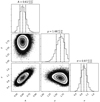 |
Fig. 1. Marginal distributions of each of the three parameters as well as the covariances between all of them. The median values and 68% confidence intervals of each of the parameters are drawn as vertical lines and also noted above the respective histograms. |
2.3. Calculating the binary fraction
Next, the model for the orbital separation distribution, with its best-fitting parameters, was used alongside the companion mass ratio distribution model from Reggiani & Meyer (2013) to calculate the binary fraction of M dwarfs as:
This calculation resulted in a binary fraction that is representative over these limited ranges of mass ratio and semi-major axis. These ranges were later expanded to [0.10 ≤ q ≤ 1.0] and [0 ≤ a < ∞ AU] to allow for the calculation of a broader M dwarf binary fraction. The error on the binary fraction was calculated as the 68% confidence interval of the probability distribution function of the binary fraction, which was generated by sampling 1000 values of A, μ, and σ from the posterior space and calculating a value of the binary fraction for each of these parameter values (as per Eq. (4)). Figure 2 summarizes the model’s fit to the data.
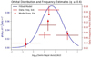 |
Fig. 2. Comparison of the binary fraction survey data to the fitted model. Each of the red horizontal lines represent one of the five binary fraction estimates from the literature. The right vertical axis position of these lines is the binary fraction reported in the data and the span along the horizontal axis of these lines is the range in semi-major axes that the respective data cover. The red vertical lines are the error in these binary fraction estimates. The blue curve is the fitted log-normal model of the orbital separation distribution. Each red dot is the binary fraction estimate obtained by integrating the fitted model over the range of semi-major axis respective to each referenced survey. When visually assessing the validity of our model, the most important aspect of this plot to notice is that each red data point fits within each red vertical line, implying that our model replicates the referenced binary fraction point estimates within the errors. |
3. Results
3.1. Orbital separation model
The best-fit to point estimates of the binary fraction from the four M dwarf surveys resulted in the parameters of A, log10(μ), and log10(σ), being 0.61 ± 0.07,  , and 0.97 ± 0.19, respectively. This fit is associated with a reduced chi-squared parameter value of 1.315. With two degrees of freedom, the probability of achieving a value greater than or equal to 1.315 is 0.269. Therefore, we could not reject the null hypothesis that the data had come from this model.
3.2. Binary fraction
Integrating Eq. (4) over the constrained regions of [0.60 ≤ q ≤ 1.00] and [0 ≤ a ≤ 10 000 AU] resulted in a binary fraction of 0.229 ± 0.028. Equation (4) was then integrated again over [0.1 ≤ q ≤ 1.0] and [0.0 ≤ a < ∞ AU] to calculate a broad binary fraction of  . This binary fraction considers stellar and sub-stellar companions to M dwarfs, but not planetary companions. The binary fraction corresponding to mass ratios and semi-major axes outside the ranges of [0.60 ≤ q ≤ 1.00] and [0 ≤ a ≤ 10 000 AU] must be considered with care because they are extrapolations of our model.
3.3. Multiplicity fraction
Due to its key role in constraining theories of stellar formation (Janson et al. 2012; De Rosa et al. 2014; Winters et al. 2019, and others), we provide an estimate of the multiplicity fraction based on our binary fraction fit. Winters et al. (2019) estimates the ratio of multiple systems (including binary and higher order systems) to binaries to be 1.179 ± 0.107 (with error propagated from the Poisson error in the number of multiple and binary systems). By assuming that the binary fraction and the total number of higher order systems are independent, we were able to multiply our binary fraction by this ratio to obtain a multiplicity fraction estimate of 0.270 ± 0.111 over the constrained regions of [0.60 ≤ q ≤ 1.00] and [0 ≤ a ≤ 10 000 AU]. The multiplicity of M dwarfs integrated over the same region of mass ratio but over all values of separation (0 − ∞) is presented here (for use in the comparison shown in Sect. 4.2) and equal to 0.272 ± 0.111.
4. Discussion
4.1. Comparisons to other M dwarf surveys
We compared our model to the observations of Bowler et al. (2015), who estimated the frequency of brown dwarf companions to M dwarf hosts. These authors observed the frequency of brown dwarf companions to M dwarf primaries over a semi-major axis range of 10−100 AU and mass ratio range of 0.039−0.224 to be  . We integrated Eq. (1) with the best fit parameters described above over these ranges of semi-major axis and mass ratio and obtained an binary fraction estimate of
  (cf. Dieterich et al. 2012). While the sample of Bowler et al. (2015) is drawn from nearby young moving groups and our preceding work was built using samples drawn from field stars, this comparison is justified because the multiplicity of stars in these moving groups does not appear to be discernibly different from the field (see Elliott et al. 2015; De Furio et al. 2019). None of the surveys used to construct our binary fraction model have probed sub-stellar companions, and so, the capability of our model to reproduce the results achieved by Bowler et al. (2015) is of particular note.
Winters et al. (2019) (W19) also studied the orbital separation distribution and binary fraction of M dwarfs. They find an upper limit to the peak in the this distribution to be at 20 AU (projected separation) and note that most stellar companions to M dwarfs lay between 4 and 20 AU. When corrected to a physical separation using the 1.26 correction factor of Fischer & Marcy (1992) (Sect. 2.1), W19’s peak to the orbital separation distribution becomes 25 AU. This falls about 1.9 standard deviations from our peak estimate of  AU (our orbital separation model estimates the probability of the peak of this distribution occurring at less than 20 AU to be about 3%). An attempt was made to draw a comparison between our binary fraction and that of W19. However, it was not shown to be a straightforward exercise to find the range of q and separation over which the survey was complete. We therefore attempted to estimate this ourselves. First, we calculated a binary fraction from the W19 sample by using their stated number of single:double:triple:high-order systems. We assumed that the binary fraction uniformly covered mass ratios from a minimum q set by the hydrogen burning limit divided by the median primary mass of their sample to a maximum q of 1. We assumed the companion mass ratio distribution of Reggiani & Meyer (2013) to convert this to the range of mass ratio that is representative of our binary fraction, 0.6−1.0. Furthermore, we assumed that the multiplicity fraction of W19 was representative for companions with separations less than 10 000 AU. However, the binary fraction that we estimated from the sample of W19, 0.133 ± 0.014 did not fall within error of our constrained binary fraction, 0.229 ± 0.028. This discrepancy is likely due to the numerous assumptions we were forced to make.
Another survey of M dwarf multiple systems, Shan et al. (2015), found the fraction of M dwarf companions with periods less than 90 days to M dwarf hosts to be  . This estimate is much higher than Delfosse et al. for closely-separated M dwarfs and would have a significant impact on our fit if it were included as a data point. However, we were unable to include Shan et al. (2015) in our analysis because the orbital separation and mass ratio completeness limits and values for each system are not easy to ascertain. Jódar et al. (2013) was also considered for inclusion in our fit but it was also not clear over what ranges of mass ratios and orbital separations this survey was complete. The microlensing survey by Shvartzvald et al. (2016) was not used in this analysis because there were difficulties in translating this work into usable point estimates without making strong assumptions that could not be verified in terms of their sensitivity limits in mass ratio and orbital separation. The inclusion of microlensing surveys would improve our analysis significantly because of their sensitivity to low-separation companions.
4.2. Comparisons to other spectral type binary fractions
We now compare the binary fraction of M dwarfs to that of sun-like FGK- and more massive A-type stars over the range of mass ratios studied here but over all separations (0.6 ≤ q ≤ 1.0 and 0.00 ≤ a ≤ ∞ AU). We expand this integration to cover all separations because of the greater prevalence of higher mass stars at larger separations. In order make this comparison, we chose an appropriate form of the companion mass ratio distribution for the stellar hosts in question, then recalculated the orbital separation distribution for each population of stars based on previous works. To make a comparison to the FGK binary fraction, we extrapolated the model of orbital separation distribution from Raghavan et al. (2010), which peaks at 48 AU, in order to integrate it over separations from 0 to ∞ AU. This was used alongside the companion mass ratio distribution of Reggiani & Meyer (2013) integrated from 0.6 to 1.0 to find an FGK-star binary fraction of 0.17 ± 0.03, where the error is estimated as the Poisson counting error based on the survey of Raghavan et al. (2010). Following the process in Sect. 3.3 of this work, we convert this binary fraction to a multiplicity fraction using the ratio of multiple systems to binary systems described in Raghavan et al. (2010) (1.33 ± 0.14) and find an FGK-star multiplicity fraction of 0.23 ± 0.14 over 0.6 ≤ q ≤ 1.0 and 0.00 ≤ a ≤ ∞ AU. We made a similar calculation for the A star binary fraction, this time based on De Rosa et al. (2014) the orbital separation distribution of this survey has a mean at nearly 400 AU). However, because the A star sample of Reggiani & Meyer (2013), which features young stars in an association, is different than that of De Rosa et al. (2014), featuring field stars, we chose to instead use the companion mass ratio distribution distribution described in De Rosa et al. (2014) to make this calculation (which is similar to that of Reggiani & Meyer 2013 at close separations but not at separations greater than 125 AU). Using this, we found an A star binary fraction of 0.11 ± 0.02 and multiplicity fraction of  by multiplying the binary fraction by the ratio of multiple systems to binary systems of De Rosa et al. (2014), 1.36 ± 0.25, over a mass ratio of 0.6 ≤ q ≤ 1.0 and orbital separation of 0.00 ≤ a ≤ ∞ AU. The binary fractions calculated here decrease as spectral type increases, but the multiplicity fractions remain consistent (with large error bars). These calculations are built on a number of assumptions; most notably, the orbital separation and companion mass ratio distributions used are complete over the entire space of 0.6 ≤ q ≤ 1.0 and 0.00 ≤ a ≤ ∞ AU. We note that the orbital separation distribution of De Rosa et al. (2014) is incomplete at low separations. In addition, the multiplicity fraction can be estimated from the binary fraction as we have done above. It is important to note that these results must be considered with these assumptions and with their large error bars in mind. This finding is in contrast to Duchêne & Kraus (2013), who suggest that the occurrence rate of companions increases with spectral type. Nonetheless, when compared over common ranges of mass ratios, the multiplicity fraction as a function of spectral type is more similar than commonly appreciated.
4.3. Additional caveats
The binary fraction study conducted here is strictly concerned with the presence of binary systems within the M dwarf population. No considerations were made to account for the presence of higher-order (triple, quadruple, etc.) systems during the fitting process. Instead, we converted the binary fraction to a multiplicity fraction using the empirical findings of other works. While such systems do exist, they are relatively rare. A recent M dwarf multiplicity study found that only 3.3% of M dwarfs exist as triple and higher-order systems (Winters et al. 2019). However, it appears that higher order systems are more common around higher mass stars (Raghavan et al. 2010; Ward-Duong et al. 2015).
Our work assumes that the mass ratio of a stellar binary system does not depend on the separation between its components (Reggiani & Meyer 2013). Moe & Di Stefano (2017) found that the distributions of mass ratio and period (which is directly proportional to separation) of O- and B-type main sequence primaries are not independent. If this is also true for M dwarf binaries, then Eq. (1) would not hold. For the time being, we accept the findings of Reggiani & Meyer (2013) but we note that further work exploring the interdependence of mass ratio and orbital separation for specifically M-type stars is needed.
Originally, our fit to the orbital separation distribution utilized the multiplicity estimate from the radial velocity data of Fischer & Marcy (1992). The inclusion of this data point (binary fraction of 0.083 ± 0.03 over 0.6 ≤ q ≤ 1 and 0.04 ≤ a ≤ 4) gave a worse fit and led to a higher reduced chi-squared value of 2.143. We believe this is due to the fact that the primary mass range of the sample of Fischer & Marcy (1992), 0.14−0.33 M⊙, does not include higher-mass M dwarfs present in the other referenced surveys. While this primary mass range may not seem substantially different from that of Delfosse et al. (1999), we examined the spectral type distributions of the parent populations of Fischer & Marcy (1992) and Delfosse et al. (1999), (Marcy & Benitz 1989; Delfosse et al. 1998, respectively), and found that they are distributed significantly differently (i.e., Marcy & Benitz 1989, and therefore Fischer & Marcy 1992, include more low mass stars than Delfosse et al. 1998, 1999) by performing a KS test and receiving a p-value of 0.0007. Previous work suggests the companion mass ratio distribution for brown dwarfs is less flat than that of M dwarfs (Burgasser et al. 2007; Fontanive et al. 2018). The inclusion of Fischer & Marcy (1992) may have been problematic because its sample is closer to the brown dwarf regime than the other referenced surveys. Therefore, we chose to exclude this point from our model fit.
5. Summary
We find that the distribution of M dwarf binary separations peaks between 33 and 66 AU within a 68% confidence interval (23−85 AU with 95 % confidence), which is comparable to the peak for FGK stars but smaller than the peak for A stars (Raghavan et al. 2010; De Rosa et al. 2014). Using the model built from this finding as well as the companion mass ratio distribution given by Reggiani & Meyer (2013), we find that the binary fraction over [0.60 ≤ q ≤ 1.00] and [0.00 ≤ a ≤ 10 000 AU] for M dwarfs to be 0.229 ± 0.028 (this is the most robust of our findings as it required the fewest extrapolations). We used this to derive the multiplicity fractions over the same range of mass ratio and over all separations for M, FGK, and A stars of 0.27 ± 0.11, 0.23 ± 0.14, and 0.15 ± 0.25 respectively. We note that these three values suggest that the multiplicity fraction is similar over these three spectral types and (within these ranges of mass ratio and orbital separation) but the error bars on these values are large. Furthermore, we find the binary fraction of M dwarfs over 0.10 ≤ q ≤ 1.00 and 0.00 ≤ a ≤ ∞ AU to be  , implying that nearly half of all M dwarfs (over all q and a) have a stellar or sub-stellar companion. This assertion is highly dependent on the validity of the assumptions we made, namely, that the frequency of binary companions is consistent beyond the parameter space of the surveys used to build our model. Data that would help improve the predictive power of our orbital separation model may include M dwarf multiplicity surveys that probe pairs with separations between 3 and 30 AU and low mass ratios. Future studies may expand upon this work by surveying the binary fraction of M dwarf companions in the brown dwarf regime, exploring correlations between the companion mass ratio and orbital separation distributions, as well as comparing M dwarf binary fraction to L, T, and Y Dwarf multiplicities.
Acknowledgments
We thank the Formation and Evolution of Planetary Systems group for their consistent support, Dr. Max Moe and Dr. Kimberly Ward-Duong for their insightful advice, and an anonymous referee whose helpful reviews significantly improved the manuscript.
References
- Bowler, B. P., Liu, M. C., Shkolnik, E. L., & Tamura, M. 2015, ApJS, 216, 7 [Google Scholar]
- Burgasser, A. J., Reid, I. N., Siegler, N., et al. 2007, in Protostars and Planets V, eds. B. Reipurth, D. Jewitt, & K. Keil, 427 [Google Scholar]
- Cortés-Contreras, M., Béjar, V. J. S., Caballero, J. A., et al. 2017, A&A, 597, A47 [NASA ADS] [CrossRef] [EDP Sciences] [Google Scholar]
- De Furio, M., Reiter, M., Meyer, M. R., et al. 2019, ApJ, 886, 95 [NASA ADS] [CrossRef] [Google Scholar]
- Delfosse, X., Forveille, T., Perrier, C., & Mayor, M. 1998, A&A, 331, 581 [NASA ADS] [Google Scholar]
- Delfosse, X., Forveille, T., Beuzit, J. L., et al. 1999, A&A, 344, 897 [NASA ADS] [Google Scholar]
- De Rosa, R. J., Patience, J., Wilson, P. A., et al. 2014, MNRAS, 437, 1216 [NASA ADS] [CrossRef] [Google Scholar]
- Dieterich, S. B., Henry, T. J., Golimowski, D. A., Krist, J. E., & Tanner, A. M. 2012, AJ, 144, 64 [Google Scholar]
- Duchêne, G., & Kraus, A. 2013, ARA&A, 51, 269 [Google Scholar]
- Dupuy, T. J., & Liu, M. C. 2011, ApJ, 733, 122 [NASA ADS] [CrossRef] [Google Scholar]
- El-Badry, K., Rix, H.-W., Tian, H., Duchêne, G., & Moe, M. 2019, MNRAS, 489, 5822 [NASA ADS] [CrossRef] [Google Scholar]
- Elliott, P., Huélamo, N., Bouy, H., et al. 2015, A&A, 580, A88 [NASA ADS] [CrossRef] [EDP Sciences] [Google Scholar]
- Fischer, D. A., & Marcy, G. W. 1992, ApJ, 396, 178 [NASA ADS] [CrossRef] [Google Scholar]
- Fontanive, C., Biller, B., Bonavita, M., & Allers, K. 2018, MNRAS, 479, 2702 [Google Scholar]
- Foreman-Mackey, D., Hogg, D. W., Lang, D., & Goodman, J. 2013, PASP, 125, 306 [Google Scholar]
- Henry, T. J., Jao, W.-C., Subasavage, J. P., et al. 2006, AJ, 132, 2360 [Google Scholar]
- Janson, M., Hormuth, F., Bergfors, C., et al. 2012, ApJ, 754, 44 [Google Scholar]
- Jódar, E., Pérez-Garrido, A., Díaz-Sánchez, A., et al. 2013, MNRAS, 429, 859 [Google Scholar]
- Marcy, G. W., & Benitz, K. J. 1989, ApJ, 344, 441 [NASA ADS] [CrossRef] [Google Scholar]
- Moe, M., & Di Stefano, R. 2017, ApJS, 230, 15 [Google Scholar]
- Raghavan, D., McAlister, H. A., Henry, T. J., et al. 2010, ApJS, 190, 1 [Google Scholar]
- Reggiani, M., & Meyer, M. R. 2013, A&A, 553, A124 [NASA ADS] [CrossRef] [EDP Sciences] [Google Scholar]
- Shan, Y., Johnson, J. A., & Morton, T. D. 2015, ApJ, 813, 75 [NASA ADS] [CrossRef] [Google Scholar]
- Shvartzvald, Y., Maoz, D., Udalski, A., et al. 2016, MNRAS, 457, 4089 [Google Scholar]
- Ward-Duong, K., Patience, J., De Rosa, R. J., et al. 2015, MNRAS, 449, 2618 [NASA ADS] [CrossRef] [Google Scholar]
- Winters, J. G., Henry, T. J., Jao, W.-C., et al. 2019, AJ, 157, 216 [NASA ADS] [CrossRef] [Google Scholar]
- Winters, J. G., Charbonneau, D., Henry, T. J., et al. 2021, AJ, 161, 63 [NASA ADS] [CrossRef] [Google Scholar]
All Tables
All Figures
|
Fig. 1. Marginal distributions of each of the three parameters as well as the covariances between all of them. The median values and 68% confidence intervals of each of the parameters are drawn as vertical lines and also noted above the respective histograms. |
| In the text | |
|
Fig. 2. Comparison of the binary fraction survey data to the fitted model. Each of the red horizontal lines represent one of the five binary fraction estimates from the literature. The right vertical axis position of these lines is the binary fraction reported in the data and the span along the horizontal axis of these lines is the range in semi-major axes that the respective data cover. The red vertical lines are the error in these binary fraction estimates. The blue curve is the fitted log-normal model of the orbital separation distribution. Each red dot is the binary fraction estimate obtained by integrating the fitted model over the range of semi-major axis respective to each referenced survey. When visually assessing the validity of our model, the most important aspect of this plot to notice is that each red data point fits within each red vertical line, implying that our model replicates the referenced binary fraction point estimates within the errors. |
| In the text | |
Current usage metrics show cumulative count of Article Views (full-text article views including HTML views, PDF and ePub downloads, according to the available data) and Abstracts Views on Vision4Press platform.
Data correspond to usage on the plateform after 2015. The current usage metrics is available 48-96 hours after online publication and is updated daily on week days.
Initial download of the metrics may take a while.