| Issue |
A&A
Volume 656, December 2021
|
|
|---|---|---|
| Article Number | A43 | |
| Number of page(s) | 11 | |
| Section | Astrophysical processes | |
| DOI | https://doi.org/10.1051/0004-6361/202141700 | |
| Published online | 02 December 2021 | |
Study of PVI-based diagnostics for 1D time-series in space plasma
1
Dipartimento di Fisica, Università di Pisa, 56127 Pisa, Italy
e-mail: This email address is being protected from spambots. You need JavaScript enabled to view it.
2
Dipartimento di Fisica, Universitá della Calabria, Via P. Bucci, 87036 Rende, Italy
3
Aix-Marseille University, CNRS, PIIM UMR 7345, 13007 Marseille, France
Received:
1
July
2021
Accepted:
7
September
2021
Abstract
Context. In the last few decades, increasing evidence has been found in both numerical studies and high-resolution in situ data that magnetic turbulence spontaneously generates coherent structures over a broad range of scales. Those structures play a key role in energy conversion because they are sites where magnetic energy is locally dissipated in plasma heating and particle energization. How much turbulent energy is dissipated via processes such as magnetic reconnection of thin coherent structures, namely current sheets, remains an open question.
Aims. We aim to develop semi-automated methods for detecting reconnection sites over multiple spatial scales. This is indeed pivotal in advancing our knowledge of plasma dissipation mechanisms and for future applications to space data.
Methods. By means of hybrid–Vlasov–Maxwell 2D–3V simulations, we combine three methods based on the partial variance of increments measured at a broad range of spatial scales and on the current density, which together, and in a synergistic way, provide indications as to the presence of sites of magnetic reconnection. We adopt the virtual satellite method, which in upcoming works will allow us to easily extend this analysis to in situ time-series.
Results. We show how combining standard threshold analysis to a 2D scalogram based on magnetic field increments represents an efficient diagnostic for recognizing reconnecting structure in 1D spatial- and time-series. This analysis can serve as input to automated machine-learning algorithms.
Key words: magnetic reconnection / turbulence / methods: numerical
© ESO 2021
1. Introduction
In the last 20 years, the launch of multi-spacecraft missions has led to great advancement of our knowledge of the main physics processes underlying the plasma dynamics in the near-Earth environment and in the solar wind. Indeed, the pioneering Cluster mission (Escoubet et al. 2001), made up of four identical spacecraft flying in a tetrahedral configuration with adjustable inter-spacecraft distance, allowed us to measure plasma fluctuations not only over a broad range of frequencies (using single-satellite data) but also as a function of spatial scale (Sahraoui et al. 2006, 2009; Narita et al. 2010). The turbulent plasma has been found to be characterized by a texture of thin discontinuities and current-sheet-like structures that spontaneously emerge at about the kinetic proton characteristic scale length (Perri et al. 2012; Greco et al. 2016). Such structures are thought to play a fundamental role in the process of magnetic energy dissipation and are often observed to be sites where magnetic reconnection occurs (Paschmann et al. 1979; Gosling et al. 2005; Øieroset et al. 2001; Vaivads et al. 2004; Retinó et al. 2007).
This picture is supported by a broad variety of numerical simulations of plasma turbulence. In particular, Servidio et al. (2011), by means of two-dimensional magnetohydrodynamic (MHD) simulations, studied the statistical relation between the detection of tangential discontinuities in the plasma and the occurrence of reconnection along a 1D path traced within the 2D simulation box. This was carried out in order to mimic the 1D measurements of a single satellite in space plasmas. It has been highlighted that tangential discontinuities characterized by very high variation in the magnetic field increments (quantitatively detected using the partial variance of increments (PVI) – see Greco et al. 2008, 2009) are very good candidates for also being identified as reconnection sites. Furthermore, both 2D and 3D kinetic simulations of collisionless plasma have pointed out that current sheets form down to the electron scale often as a result of local instabilities and are characterized by strong local dissipation and plasma heating (Karimabadi et al. 2013; Wan et al. 2015; Arró et al. 2020). These thin current sheets have also been proposed as a competitive mechanism, with respect to the standard MHD turbulent cascade, for injecting the energy at smaller subion scales. In other words, the plasma turbulence cascade from intermediate to proton scales is also mediated by the formation of a huge number of current-sheet structures subsequently disrupted by fast reconnection (Cerri & Califano 2017; Franci et al. 2017).
Moreover, hybrid–Vlasov–Maxwell (HVM) experiments also show regions characterized by high values of the current density, high vorticity, and heat associated to ion temperature anisotropy and distorted particle velocity distribution functions (VDFs) that highly deviate from the initially imposed Maxwellian equilibrium (Greco et al. 2012; Valentini et al. 2016). These experiments point out the occurrence of strong interactions between turbulent fields and particles. Haynes et al. (2014) in 2D particle-in-cell (PIC) simulations detected reconnection sites close to magnetic field X-points associated to parallel electron temperature anisotropy and multi-peaked electron VDFs.
These coherent structures and reconnection sites, first identified in numerical experiments as regions of localized plasma energy dissipation, have been directly studied in near-Earth plasmas thanks to the Magnetosphere MultiScale (MMS) mission. This mission was specifically designed to identify ion and electron diffusion regions in the terrestrial magnetospheric plasma, as well as to study the impact of small-scale plasma turbulence on the acceleration and heating of particles. Indeed, the distance between the four satellites can reach about 10 km, corresponding there to about the electron scale, a distance never reached before (Burch et al. 2015; Eriksson et al. 2016; Ergun et al. 2016; Vörös et al. 2017). In particular, the very high-resolution data from the Fast Plasma Investigation instrument on board MMS (Pollock et al. 2016) have allowed identification of strong distortions of the ion and electron VDFs and local heating close to reconnection sites and coherent structures at subproton scales (Burch et al. 2015; Yordanova et al. 2016; Graham et al. 2017; Chasapis et al. 2017).
In the present work, we aim to identify coherent structures at proton and subproton scales resulting from 1D time-series obtained with the virtual satellite technique from a 2D HVM numerical experiment. To this purpose, we set up a semi-automated method based on the computation of the partial variance of increments (Greco et al. 2018). This allows us to determine the possible presence of reconnecting structures.
2. Methods
2.1. Simulation
We performed a 2D–3V HVM simulation of plasma turbulence across the ion cyclotron frequency. In this model, ions are fully kinetic while electrons are assumed to take the form of a neutralizing isothermal fluid with mass through a generalized Ohm’s law (Valentini et al. 2007). The dimensionless HVM system of equations is summarized as follows. The Vlasov equation for the ion distribution function fi = fi(x, v, t) is given by,
 (1)
(1)
where E and B are the electric and magnetic field. The Ohm’s equation for the electron response reads,
 (2)
(2)
where  is the fluid velocity, with ui and ue being the ion and electron fluid velocity, respectively. Finally, the Ampère and Faraday laws read,
 (3)
(3)
where the current displacement has been neglected in the Ampére law and quasi-neutrality, ni ≃ ne ≡ n has been assumed. The ion density ni and the ion fluid velocity ui are calculated as the zeroth and first-order velocity momentum of fi, respectively. All equations are normalized to the ion mass mi, the ion cyclotron frequency Ωci = eB0/mic (B0 is the initial mean magnetic field), the Alfvén velocity  (n0 is the initial mean ion density), and the ion skin depth di = vA/Ωci. With these normalizations, the electron skin depth is given by
  , where me is the electron mass. For the electron pressure, we take an isothermal equation of state: Pe = nT0, e. The set of Eqs. (1)–(3) is solved in a 2D–3V phase space using an Eulerian algorithm (Mangeney et al. 2002) which combines the so-called splitting scheme with the current advanced method (for details, see Valentini et al. 2007). Our squared numerical box of side L = 100π is sampled by Nx × Ny = 3072 × 3072 uniformly distributed grid points corresponding to Δx = Δy ∼ 0.1di. We set the initial mean field along z with modulus B0 = 1. The initial distribution function is a Maxwellian of uniform temperature T0i = T0e and the ion beta βi = 1. The velocity space is sampled by 513 uniformly distributed grid points spanning [ − 5vth, i, 5vth, i] in each direction, where
  is the initial ion thermal velocity. We set the reduced mass ratio mi/me = 100 so that di and de are sufficiently separated. Turbulence is initialized by adding random, isotropic magnetic-field perturbations to the equilibrium configuration with wave-number lying in the interval k ∈ [0.02, 0.12] and a root mean squared value for the magnetic field fluctuations of δBrms ∼ 0.28 (for a detailed discussion on the initial conditions, see Califano et al. 2020). The wavelengths of the initial perturbation wave packet correspond to the largest allowed by the numerical box.
The dynamical evolution at play in our simulation is summarized in Fig. 1 by three snapshots of the current density magnitude J ≡ |J| at different times, t = 20, 247, 494 (hereafter in  units). In the initial phase (shown in the left panel) the fluctuations injected at large scales start to interact nonlinearly and set up the initial phase of the energy cascade. As a result, after about one eddy turnover time, t ∼ 247, an intermediate phase is reached (middle panel in Fig. 1) where we observe the presence of several well-defined, thin and elongated current sheets (CSs). In a number of these CSs, magnetic reconnection occurs eventually efficiently injecting the energy at subion scales. After about two eddy turnover times, t ∼ 494 (right panel in Fig. 1), the system reaches the final phase where turbulence is now fully developed. The fully developed turbulence state is highlighted by the time-evolution of the root mean square of the current density,
  reaching its peak value. Correspondingly, we observe the development of a typical power-law turbulent spectrum shown in Fig. 2 (see e.g., Cerri et al. 2016).
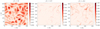 |
Fig. 1. Distribution of the intensity of the current density within the x–y plane at three different simulation times (indicated at the top of the panels). The time t = 494 corresponds to a fully developed turbulent state, where a Kolmogorov-like spectrum at intermediate scales has developed (see Fig. 2). |
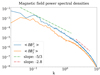 |
Fig. 2. Magnetic field power spectral densities at t ∼ 494 for the magnetic field component within the x–y plane (blue line), and for the out-of-plane magnetic field component (orange line). The Kolmogorov-like trend for wavenumbers smaller than the one corresponding to the ion scale is also shown (green dashed line), as well as a k−2.8 power law at higher wavenumbers (red dashed line) to guide the eye. |
2.2. Sampling 2D turbulent structures along a 1D path
For the present analysis, we consider the state of the system during the intermediate and final states, namely at t = 247, and at t = 494. We allow a virtual satellite to “fly” within the 2D simulation box, that is we track a 1D path within a 2D snapshot of the fields. This has been implemented by interpolating the simulation data along a selected path. When a path reaches the boundary of the simulation box, the virtual satellite re-enters the box from the opposite side following the simulation periodicity. This technique has been extensively used by Greco et al. (2012) and Donato et al. (2013). We selected different trajectories for the virtual spacecraft crossing the box at different angles with respect to the x-axis in order to maximize the probability of crossing emerging current sheets and coherent structures in the turbulent field. An example is reported in Fig. 3 where the artificial 1D satellite path (blue line) samples a highly structured current density. Such a trajectory forms an angle α = 5° with respect to the x-axis.
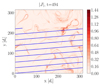 |
Fig. 3. Example of a 1D virtual satellite path within the simulation box at an angle α = 5° with respect to the x axis. |
Along such a 1D path we calculated the so-called partial variance of increments (PVI) (Greco et al. 2008, 2018), defined as:
 (4)
(4)
where ΔB(s, Δs) = B(s + Δs)−B(s) represents the magnetic field vector increments calculated between points along the 1D trajectory s separated by a lag scale Δs. Here ⟨ ⋅ ⟩ indicates the average value along the entire 1D path. Such a technique allows us to directly compare PVI space-series resulting from the virtual satellite with the PVI time-series from real spacecraft, under the assumption that the evolution time of the turbulence in real space is much longer than the advection time of the plasma bulk flow passing through the spacecraft. Indeed, under this “frozen-in” assumption (Taylor 1938) it is possible to transform time-series from satellites into space-series (being s = Vbulkt).
We computed the following analysis choosing trajectories at angles: 5°, 8°, 13°, 75°, 80°, and 85°. At t ∼ 247 we also take α = 33° and 78°, while at t ∼ 494 we also considered α = 18°, 34°, and 45° in order to cross X-points emerging from the turbulent field.
3. Results
3.1. Statistical analysis
Following Servidio et al. (2011) and Donato et al. (2013), we explored the correlation between reconnection sites and high PVI events in a regime where we observe the development of thin current sheets over scales comparable with the ion skin depth.
In MHD and Hall-MHD numerical simulations, Servidio et al. (2011) and Donato et al. (2013) applied an arbitrary threshold θ on the PVI signal by imposing that ℐ(Δs, s) > θ. They found a direct correlation between PVI events that satisfy the threshold method and reconnection sites. Thus, they defined two quantities called goodness and efficiency. The former is the number of the successes (reconnection events) over the total number of identified discontinuities via the threshold method, while the latter is the ratio of the number of identified reconnection sites to the total number of reconnection regions along the trajectory. It has been found that the goodness increases as the PVI threshold increases, while efficiency decreases. Osman et al. (2014) applied a similar PVI-threshold methodology (at fixed lag scales Δs) to solar wind data from the Wind spacecraft at 1 AU, obtaining the same trend (the higher the threshold, the higher the goodness but the lower the efficiency). As higher values of PVI are related to the presence of intermittent structures in a turbulent environment, the observed trend of goodness implies that reconnecting events tend to have a more intermittent character than nonreconnecting ones.
In our simulations, we selected a set of “verified” reconnection events using a threshold on the current density defined as in Uritsky et al. (2010). We further checked the selected current sheets one by one by looking at reconnection signatures in the current density, electron decoupling, electron vorticity, Hall field, in-plane magnetic field, and the electron outflows. We then interpolated the virtual spacecraft trajectories at various angles crossing the above selected reconnecting current sheets.
We performed the statistical analysis at t = 247 and t = 494. Moreover, we compute the PVI as in Eq. (4) at 60 different spatial scales, ranging from Δs = 0.05di to Δs = 3di. Following the methodology outlined above, we computed the goodness by selecting different PVI thresholds. We express the threshold θ for a given quantity Q as the number n of standard deviations σ from the mean value μ, that is θ(Q) = μ(Q)+nσ(Q) with μ(Q) = ⟨Q⟩ and  . Thus, the threshold computed for the standardized PVI (ℐ − μ(ℐ))/σ(ℐ) is of a very simplified form, namely (θ − μ)/σ = n. This is extremely useful when working with multiple series of data, each with its own statistics. Figures 4 and 5 show the results of this analysis at t = 247 and t = 494, respectively. At both times, the goodness increases as the PVI threshold increases, reaching values of > 80% for thresholds > μ + 10σ. This goodness–threshold relation is particularly evident if we consider the variation of goodness at a fixed scale for different thresholds as in Fig. 6 (solid lines). Thus, our findings corroborate the idea that reconnecting current sheets are more intermittent than nonreconnecting ones. Also in Fig. 6 the number of PVI peaks above a given threshold is reported (dotted lines), which is the denominator for the goodness. By increasing the threshold value, the number of PVI events above the threshold decreases, affecting the statistical significance of the goodness. For this reason, we consider PVI thresholds θ ≤ μ + 18σ.
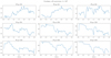 |
Fig. 4. For t = 247 values of the goodness as a function of the spatial scale in units of di, for nine different PVI thresholds, corresponding to the nine panels. At this time, the typical size of the current sheets is ∼1 di. It is worth mentioning that at this stage of the simulation the PVI is a good indicator of reconnecting current sheets over a broad range of scales. |
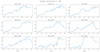 |
Fig. 5. For t = 494 values of the goodness as a function of the spatial scale in units of di, for nine different PVI thresholds, corresponding to the nine panels. We note that in such a state of fully developed turbulence, the typical size of the emerging current sheets is 0.85di. For structures greater in size than this typical scale, the goodness starts increasing and is higher for larger PVI thresholds (in agreement with Servidio et al. 2011). |
A scale dependence is observed both at t = 247 (see Fig. 4) and in the fully developed state t = 494 (see Fig. 5). This dependence has to be ascribed to the multi-scale character of a fully developed turbulent plasma. We note that, at t = 494, at scales smaller than about 1di the goodness tends to decrease. This evidence can be explained by the fact that the HVM simulation allows for the formation of structures smaller than di that are not reconnecting current sheets but thin discontinuities or interfaces between different portions of plasma. We show examples of this kind of discontinuity in the following section, together with other diagnostics that complement the goodness method in the detection of reconnecting current sheets.
To complement the present analysis, we gathered information about the PVI peak values of the human-verified events. We found 19 human-identified reconnection regions at t = 247 and 47 at t = 494. These sites are identified as 2D regions in the whole simulation box. The virtual spacecraft can cross these reconnection sites multiple times. We collect the PVI peak values for all scales Δs each time a region labeled as a reconnection is crossed. In Fig. 7, for each Δs, we show the mean value of these PVI peaks (blue squares) along with the ±1 standard deviation interval (blue vertical bar) and their extreme values (upright and upside-down black triangles). This is done separately at t = 247 and t = 494. It can be observed that by increasing the threshold value, the number of reconnecting sites decreases but the total number of above-threshold events also decreases (see also Fig. 6). The former is the numerator and the latter the denominator of the goodness. Overall, this leads to an increase in the goodness values (as found in previous studies and already discussed). From Fig. 7, we observe that the PVI peaks related to the human-labeled reconnection regions at t = 247 are larger than those found at t = 494. This suggests that reconnection structures are “sharper” at t = 247 before the fully developed turbulence is reached. Assuming that this is correlated with the thickness of the reconnecting current sheets, we should expect faster (on average) reconnection at t = 247. For t = 494, we also observe a constant rise in the max PVI peak value (upright triangles) at high scales (Δs > 2). This is probably linked to the concomitant formation of reconnecting structures at larger scales due to the turbulent cascade process.
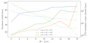 |
Fig. 6. Solid lines: Variation of goodness as a function of threshold θ in three different cases: (1) Δs = 1.5di, t = 247; (2) Δs = 1.5di, t = 494; and (3) Δs = 2.5di, t = 494. Dotted lines: Number of PVI peaks above each threshold value for the same three cases (in matching colors). |
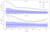 |
Fig. 7. Average of the PVI peak values related to the human-verified reconnection events (i.e., average of the PVI local maxima collected at each crossing of reconnection regions) for each lag Δs (blue squares). The ±1σ interval (blue vertical bars), the maximum values (upright black triangles), and the minimum values (upside-down black triangles) are also reported. Horizontal dashed lines are the thresholds used for Figs. 4–5. To compare PVI peak values from different trajectories, the standardized PVI (ℐ − μ(ℐ))/σ(ℐ) is reported (where μ(ℐ) = ⟨ℐ⟩). Top panel is for t = 247 and the bottom panel for t = 494. |
We investigated the possible joint use of the current density measurement and of the PVI as proxies for magnetic reconnection. In particular, we considered the PVI signal over the virtual satellite trajectory integrated over all the spatial scales considered, namely ∫Δsℐ. The choice of this second quantity is done for both practical and physical reasons. The practical reason is the resultant reduction of proxies to be worked with, as all the Δs-dependent PVI series are “cumulated” into the Δs-integrated ones. An alternative approach would be to select a single Δs for the entire analysis. However, as discussed in Sect. 3.2, during magnetic reconnection we expect a broad range of scales to be involved, and this is the physical reason for the use of ∫Δsℐ. Therefore, we set different thresholds on both J2 and ∫Δsℐ in order to find an optimal combination. We set
 (5)
(5)
 (6)
(6)
Then, from all the trajectories, segments of length Δs = 3.066di (the largest PVI scale considered) are extracted if they satisfy at least one of the following requirements: (i) one or more points belong to a structure human-labeled as “reconnection”, (ii) in one or more points J2 > θ(J2), and/or (iii) in one or more points ∫Δsℐ > θ(∫Δsℐ).
Thanks to the human-labeling and to the two thresholds, it is possible to subdivide them into true positives (TP), false positives (FP), and false negatives (FN). Thus, we can compute the goodness as TP/(TP + FP) and the efficiency as TP/(TP + FN). To balance these two indicators, we used the F1 score, which is the harmonic mean of the two:
 (7)
(7)
It is important to indicate the condition that distinguishes positives from negatives. Having two thresholds, we have four possibilities: (i) consider as positive any segment where at least one of the two thresholds is exceeded, (ii) consider a segment positive only if both thresholds are exceeded, (iii) consider a segment positive if the threshold on J2 is exceeded, or (iv) consider a segment positive if the threshold on ∫Δsℐ is exceeded. Both (iii) and (iv) are trivial cases of this double-threshold analysis. We found that option (ii) maximizes the F1 score with the threshold pairs (μ(J2)+4σ(J2),μ(∫Δsℐ)+6σ(∫Δsℐ)). However, the F1 score obtained is just 0.58 and cannot be considered as satisfying.
In the following section we further analyze trajectory segments using the above pair of thresholds (μ(J2)+4σ(J2),μ(∫Δsℐ)+6σ(∫Δsℐ)) and complementing the F1 score analysis with PVI scalograms.
3.2. Scalogram analysis
It is hard to recognise what kind of structure is crossed simply by analyzing a 1D time-series. In order to obtain more physical information on the structures embedded in the plasma and crossed by the satellite, it is possible to study time-series using a 2D scalogram with scale and space dependencies.
This can be done by applying a wavelet transform to the 1D signal. However, as discussed in Vörös et al. (2010), the fact that the same wavelet basis has to be applied to the whole series can generate erroneous representations if the signal presents sudden jumps and strong nonlinearity. Wavelet analysis can be adopted successfully for nonlinear systems, but it heavily depends on the choice of the mother wavelet, proper resolution, and scale discretization.
Alternatively, one can obtain scalograms using the PVI computed over the trajectory at different scales. This was implemented by Greco et al. (2016) in the context of magnetic reconnection in turbulent plasma using data from the Cluster satellites. Here, we apply that method on our 2D simulated fields. At different times, we trace several 1D trajectories over the box, allowing for a relatively large sampling in the form of space series.
In Fig. 8, the gray dotted line represents one of these trajectories in the simulation box at time t = 247. All structures of interest are reported along the trajectory: reconnecting regions are indicated by red circles, green circles indicate points where  (as the threshold is still computed from J2), and blue dots are points where the scale-integrated PVI overcomes its threshold, μ(∫Δsℐ)+6σ(∫Δsℐ). Once again, the threshold values are obtained by maximizing the F1 score, that is, by taking a segment as positive only if both thresholds are exceeded. This method to define positives and negatives is used in what follows.
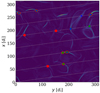 |
Fig. 8. Example of a virtual satellite trajectory (t = 247 and α = 8°). Sites of magnetic reconnection are localized by red circles, sites where ∫Δsℐ > θ(∫Δsℐ) are localized by green circles, and sites where J2 > θ(J2) are localized by blue circles. |
In the PVI scalogram, over the entire virtual satellite trajectory (not shown here), there are portions of the signal characterized by high values. Such regions need to be studied separately. Examples of structures crossed by the virtual satellite are analyzed below.
Figure 9 shows three crossed plasma structures in detail. Time-series of the intensity of the current density J (green) and of the scale-integrated PVI ∫Δsℐ (blue) are displayed in the top panels, together with the two respective thresholds (dashed lines). Red regions indicate reconnection sites as detected from the analysis in Sect. 3.1 (i.e., human-labeling). The bottom panel presents the PVI scalogram over the segment.
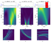 |
Fig. 9. (a) Simple turbulence crossing (t = 494, α = 85°). (b) Boundary of magnetic structure with strong shear, but no reconnection (t = 247, α = 33°). (a) and (b) structures have been selected via the threshold on J only (true negatives). (c) Crossing of a reconnection separatrix (t = 494, α = 85°), selected via the threshold on J and on the scale-integrated PVI, as well as using human labeling (true positive). See text for further details. (d–f) Overview of the structures crossed in the 2D box. |
As expected, the scale-integrated PVI and the electric current intensity tend to be well correlated along the trajectories (Greco et al. 2016). Also, regions human-labeled as reconnections coincide with large-amplitude peaks in both quantities. An analysis performed over all the trajectory segments suggests that those in which only the ∫Δsℐ overcomes the threshold are never (or rarely) labeled by human as reconnecting. This means that the scale-integrated PVI is not a precise reconnection proxy if used alone. Regions human-labeled as reconnecting with both ∫Δsℐ and J under their thresholds correspond to reconnection structures that are too small to be adequately resolved by the simulation grid or too feeble to be of particular interest. Moreover, it is plausible that these small and/or feeble structures are more prone to human mislabeling.
Figures 9a and b show two typical examples of nonreconnecting regions selected using a threshold on J. Figure 9a shows a virtual satellite crossing of the turbulent plasma (cf. Fig. 9d). In this example, all scales are involved, but thanks to the spatial information in the PVI scalogram one can see that there is no clear pattern that can be linked to a specific structure. On the other hand, in Fig. 9b the PVI scalogram very clearly shows the boundary region of the selected magnetic structure (cf. Fig. 9e), which is characterized by high values of PVI. The boundary is highly localized both in space and in scale. This corresponds to the edge of an island where a strong shear is present but without reconnection. We noticed that, in our numerical simulation, nonreconnecting structures tend to have the current overcoming its threshold but not the scale-integrated PVI. In summary, the single threshold analysis on the current density or on the scale-integrated PVI generates many false positives (especially on the current), while the double threshold analysis is able to cut out many of those false positives.
Figure 9c represents a crossing of a single separatrix1 close to a reconnection region (cf. Fig. 9f) localized using both the threshold methods on PVI and J, and the human-labeling (i.e., a true positive). PVI tends to be quite high over a broad range of scales and slightly shifted with respect to the peak in J. This happens because the separatrix region is characterized by an internal structure where turbulence starts developing. More importantly, all scales are involved.
In Fig. 10a (also a true positive), both separatrices (relative to the same outflow) are crossed (cf. Fig. 10d). Again, magnetic energy is spread over a broad range of scales, and the PVI scalogram unveils an internal structure of the outflow region. Two space-localized peaks in the PVI scalogram that are well separated at small scales drift until they merge at larger scales. We note that scale-integrated PVI values are above the threshold. Figure 10b (true positive) displays a similar two-separatrices crossing, but this time closer to the X-point of the diffusion region (cf. Fig. 10e). The pattern in the PVI scalogram presents, again, two spatially separated peaks at small scales that drift until they merge. After the merging, the pattern develops in a 2D cone, opening toward high scales. This pattern can be considered as representative of a crossing of a magnetic reconnecting region.
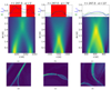 |
Fig. 10. (a) Crossing of two reconnection separatrices at a certain distance from the X-point (t = 247, α = 5°), selected via the threshold on |J| and on the scale-integrated PVI, as well as using human labeling (true positive). (b) Crossing of two separatrices close to the X-point of a reconnecting region (t = 247, α = 78°), which is again a true positive. (c) Crossing of two separatrices (t = 247, α = 13°) selected via the threshold method on J and on PVI, but not via human labeling (i.e., false positive). (d–f) Overview of the structures crossed in the 2D box. |
Figure 10c corresponds to a reconnecting structure, albeit quite deformed by the turbulent dynamics (cf. Fig. 10f), crossed by the virtual spacecraft, and classified as a false positive (both current and PVI are above their thresholds, but the site was not labeled as reconnection). The PVI scalogram shows the typical pattern of a two-separatrices crossing, similar to Fig. 10a. This suggests that the method of the “drift-cone” pattern (or class of patterns) can be very useful in searching for reconnecting structures from 1D time-series. Indeed, we found that this approach turns out to be very effective even in cases where it is hard for humans to discern the occurrence of reconnection or not.
In Fig. 11a we show a typical electron diffusion region (EDR) crossing, which is characterized by a large-amplitude scale-integrated PVI peak symmetric with respect to the EDR crossing point (cf. Fig. 11d). In this case, the PVI scalogram has a cone-like pattern over all scales. This feature may depend on the actual crossing angle (with respect to the neutral line) of the structure. Thus, in Fig. 11b we capture a normal (with respect to the neutral line) EDR crossing (cf. Fig. 11e). The PVI scalogram shows the same cone-like pattern. A symmetric scale-integrated PVI peak is also found, even if lower in amplitude with respect to the previous one. This can be very useful for understanding how a satellite is crossing a diffusion region. Both crossings are true positives.
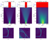 |
Fig. 11. (a) Typical X-point crossing (t = 247, α = 13°). (b) Normal crossing of an X-point (t = 494, α = 34°). Both sites are true positives. (c) Longitudinal crossing of an X-point (t = 247, α = 85°), which is a false negative because the scale-integrated PVI is under threshold. (d–f) Overview of the structures crossed in the 2D box. |
A more peculiar EDR crossing is shown in Fig. 11c. Here, the crossing is quasi-longitudinal, that is, quasi-parallel to the neutral line (cf. Fig. 11f). The cone-like pattern is still present, but the PVI amplitude decreases drastically and no peak is found in the scale-integrated PVI. This suggests that the pattern in the PVI scalogram could be a more robust proxy with respect to the threshold methods (Greco et al. 2008, 2009). Indeed, this site is a false negative because the scale-integrated PVI is under threshold but the PVI scalogram clearly hints that it is an EDR crossing.
PVI scalograms can also help to filter away some false positives, which are the major issue in the “double-threshold” analysis presented in the previous Section. Figure 12a shows a turbulent structure crossing that has been flagged as positive because both quantities are over their thresholds (cf. Fig. 12b). However, a quick look at the PVI scalogram shows that no particular patterns across the spatial scales are present.
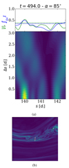 |
Fig. 12. (a) Crossing of a turbulent region (t = 494, α = 85°) detected as a positive by the double-threshold method, but with no features in the PVI scalogram (i.e., false positive). (b) Overview of the structure crossed in the 2D box. |
4. Conclusions
In order to detect reconnection sites in 1D time- and space-series sampled by a (virtual) satellite flying into a HVM simulation, we considered three different diagnostics. The first two are standard threshold methods applied to the intensity of the current density and to the PVI signals (considered both per-scale and scale-integrated). The third one is the PVI scalogram as a function of the time and space trajectories of the spacecraft and of the spatial scales and timescales. PVI scalograms were successfully applied to Cluster data set to detect the presence of coherent magnetized structures characterized by a broad range of timescales (Greco et al. 2016). Typically, the PVI threshold method can capture all structures emerging from the turbulent dynamics, such as magnetic field inhomogeneity, magnetic discontinuities, and vortices, which are often sites of local energy conversion (Servidio et al. 2012; Perrone et al. 2020; Fadanelli et al. 2021).
The main achievements of the present analysis are the following.
-
Using the threshold method on J and on the scale-integrated PVI is not sufficient to localize a reconnection site because these methods strongly depend on the way the satellite crosses the reconnecting structure (see e.g., Figs. 11f and c).
-
When the satellite crosses a reconnecting current sheet, the PVI scalogram exhibits a typical cone-like pattern extending over a broad range of scales. Depending on how the structure is crossed by the spacecraft, it can also show an X-shaped pattern.
-
Nonreconnecting sites can have J and the PVI above their arbitrary thresholds, but the scalogram does not exhibit any particular feature (see Fig. 12a).
This combined analysis method turns out to be very effective and can be straightforwardly extended to in situ spacecraft time-series. As far as spacecraft data are concerned, the computation of PVI scalograms from 1D time-series was found to be a powerful method of investigation. Indeed, it only requires high-resolution magnetic field data, which are relatively easily obtained by modern space missions (Balogh et al. 2001; Burch et al. 2015; Fox et al. 2016; Horbury et al. 2020). On the other hand, computing current density from in situ data is often challenging, because it implies either the presence of a multi-spacecraft fleet (typically a constellation of four satellites; Dunlop et al. 2002) or high-cadence plasma data that relate the current density to plasma density and to ion and electron speeds (see also Perri et al. 2017). Thus, recognizing signatures of magnetic reconnection regions in PVI scalograms can be an easy tool to implement for single-spacecraft missions but also in cases where high-resolution plasma data are not available. We plan to extensively apply this method to already studied reconnection regions detected by MMS at 1 AU (Burch et al. 2015; Ergun et al. 2016; Vörös et al. 2017) and to new data sets from Parker Solar Probe and Solar Orbiter, in order to improve our knowledge on the rate of occurrence of reconnecting structures as a function of the radial distance from the Sun. Further, it is worth mentioning the fact that the joint results from these three methods can be passed as input to machine learning algorithms. We indeed advocate the use of the PVI scalogram analysis in the framework of an algorithmic strategy in order to automatize the classification process. The most obvious way to do this would be to use a convolutional neural network (CNN); this strategy is widely adopted in image recognition, and was used for the specific case of magnetic reconnection in Hu et al. (2020).
Acknowledgments
This work has received funding from the European Unions Horizon 2020 research and innovation programme under grant agreement No. 776262 (AIDA, http://www.aida-space.eu). Numerical simulations have been performed on Marconi at CINECA (Italy) under the ISCRA initiative. FC thanks Dr. M. Guarrasi (CINECA, Italy) for his contribution on code implementation on Marconi.
References
- Arró, G., Califano, F., & Lapenta, G. 2020, A&A, 642, A45 [NASA ADS] [CrossRef] [EDP Sciences] [Google Scholar]
- Balogh, A., Carr, C. M., Acuña, M. H., et al. 2001, Ann. Geophys., 19, 1207 [NASA ADS] [CrossRef] [Google Scholar]
- Burch, J., Moore, T., Torbert, R., & Giles, B. 2015, Space Sci. Rev., 199 [Google Scholar]
- Califano, F., Cerri, S. S., Faganello, M., et al. 2020, Front. Phys., 8, 317 [NASA ADS] [CrossRef] [Google Scholar]
- Cerri, S. S., & Califano, F. 2017, New J. Phys., 19, 025007 [NASA ADS] [CrossRef] [Google Scholar]
- Cerri, S. S., Califano, F., Jenko, F., Told, D., & Rincon, F. 2016, ApJ, 822, L12 [NASA ADS] [CrossRef] [Google Scholar]
- Chasapis, A., Matthaeus, W. H., Parashar, T. N., et al. 2017, ApJ, 836, 247 [NASA ADS] [CrossRef] [Google Scholar]
- Donato, S., Greco, A., Matthaeus, W. H., Servidio, S., & Dmitruk, P. 2013, J. Geophys. Res. (Space Phys.), 118, 4033 [NASA ADS] [CrossRef] [Google Scholar]
- Dunlop, M. W., Balogh, A., Glassmeier, K. H., & Robert, P. 2002, J. Geophys. Res. (Space Phys.), 107, 1384 [NASA ADS] [CrossRef] [Google Scholar]
- Ergun, R. E., Goodrich, K. A., Wilder, F. D., et al. 2016, Phys. Rev. Lett., 116, 235102 [NASA ADS] [CrossRef] [Google Scholar]
- Eriksson, S., Wilder, F. D., Ergun, R. E., et al. 2016, Phys. Rev. Lett., 117, 015001 [NASA ADS] [CrossRef] [Google Scholar]
- Escoubet, C. P., Fehringer, M., & Goldstein, M. 2001, Ann. Geophys., 19, 1197 [NASA ADS] [CrossRef] [Google Scholar]
- Fadanelli, S., Lavraud, B., Califano, F., et al. 2021, J. Geophys. Res. (Space Phys.), 126, e28333 [NASA ADS] [Google Scholar]
- Fox, N. J., Velli, M. C., Bale, S. D., et al. 2016, Space Sci. Rev., 204, 7 [Google Scholar]
- Franci, L., Cerri, S. S., Califano, F., et al. 2017, ApJ, 850, L16 [NASA ADS] [CrossRef] [Google Scholar]
- Gosling, J. T., Skoug, R. M., McComas, D. J., & Smith, C. W. 2005, J. Geophys. Res. (Space Phys.), 110, A01107 [Google Scholar]
- Graham, D. B., Khotyaintsev, Y. V., Vaivads, A., et al. 2017, Phys. Rev. Lett., 119, 025101 [CrossRef] [Google Scholar]
- Greco, A., Chuychai, P., Matthaeus, W. H., Servidio, S., & Dmitruk, P. 2008, Geophys. Res. Lett., 35, L19111 [Google Scholar]
- Greco, A., Matthaeus, W. H., Servidio, S., Chuychai, P., & Dmitruk, P. 2009, ApJ, 691, L111 [Google Scholar]
- Greco, A., Valentini, F., Servidio, S., & Matthaeus, W. H. 2012, Phys. Rev. E, 86, 066405 [NASA ADS] [CrossRef] [Google Scholar]
- Greco, A., Perri, S., Servidio, S., Yordanova, E., & Veltri, P. 2016, ApJ, 823, L39 [CrossRef] [Google Scholar]
- Greco, A., Matthaeus, W. H., Perri, S., et al. 2018, Space Sci. Rev., 214, 1 [NASA ADS] [CrossRef] [Google Scholar]
- Haynes, C. T., Burgess, D., & Camporeale, E. 2014, ApJ, 783, 38 [NASA ADS] [CrossRef] [Google Scholar]
- Horbury, T. S., O’Brien, H., Carrasco Blazquez, I., et al. 2020, A&A, 642, A9 [NASA ADS] [CrossRef] [EDP Sciences] [Google Scholar]
- Hu, A., Sisti, M., Finelli, F., et al. 2020, ApJ, 900, 86 [NASA ADS] [CrossRef] [Google Scholar]
- Karimabadi, H., Roytershteyn, V., Wan, M., et al. 2013, Phys. Plasmas, 20, 012303 [Google Scholar]
- Mangeney, A., Califano, F., Cavazzoni, C., & Travnicek, P. 2002, J. Comput. Phys., 179, 495 [NASA ADS] [CrossRef] [Google Scholar]
- Narita, Y., Sahraoui, F., Goldstein, M. L., & Glassmeier, K. H. 2010, J. Geophys. Res. (Space Phys.), 115, A04101 [Google Scholar]
- Øieroset, M., Phan, T. D., Fujimoto, M., Lin, R. P., & Lepping, R. P. 2001, Nature, 412, 414 [CrossRef] [Google Scholar]
- Osman, K. T., Matthaeus, W. H., Gosling, J. T., et al. 2014, Phys. Rev. Lett., 112, 215002 [NASA ADS] [CrossRef] [Google Scholar]
- Paschmann, G., Papamastorakis, I., Sckopke, N., et al. 1979, Nature, 282, 243 [CrossRef] [Google Scholar]
- Perri, S., Goldstein, M. L., Dorelli, J. C., & Sahraoui, F. 2012, Phys. Rev. Lett., 109, 191101 [NASA ADS] [CrossRef] [Google Scholar]
- Perri, S., Valentini, F., Sorriso-Valvo, L., Reda, A., & Malara, F. 2017, Planet. Space Sci., 140, 6 [NASA ADS] [CrossRef] [Google Scholar]
- Perrone, D., Bruno, R., D’Amicis, R., et al. 2020, ApJ, 905, 142 [NASA ADS] [CrossRef] [Google Scholar]
- Pollock, C., Moore, T., Jacques, A., et al. 2016, Space Sci. Rev., 199, 331 [CrossRef] [Google Scholar]
- Retinó, A., Sundkvist, D., Vaivads, A., et al. 2007, Nat. Phys., 3, 235 [CrossRef] [Google Scholar]
- Sahraoui, F., Belmont, G., Rezeau, L., et al. 2006, Phys. Rev. Lett., 96, 075002 [CrossRef] [Google Scholar]
- Sahraoui, F., Goldstein, M. L., Robert, P., & Khotyaintsev, Y. V. 2009, Phys. Rev. Lett., 102, 231102 [NASA ADS] [CrossRef] [Google Scholar]
- Servidio, S., Greco, A., Matthaeus, W. H., Osman, K. T., & Dmitruk, P. 2011, J. Geophys. Res. (Space Phys.), 116, A09102 [Google Scholar]
- Servidio, S., Valentini, F., Califano, F., & Veltri, P. 2012, Phys. Rev. Lett., 108, 045001 [NASA ADS] [CrossRef] [Google Scholar]
- Taylor, G. I. 1938, Proc. R. Soc. Lond. Ser. A, 164, 476 [NASA ADS] [CrossRef] [Google Scholar]
- Uritsky, V., Pouquet, A., Rosenberg, D., Mininni, P., & Donovan, E. 2010, Phys. Rev. E Stat. Nonlinear Soft Matter Phys., 82, 056326 [Google Scholar]
- Vaivads, A., Khotyaintsev, Y., André, M., et al. 2004, Phys. Rev. Lett., 93, 105001 [NASA ADS] [CrossRef] [Google Scholar]
- Valentini, F., Califano, F., Hellinger, P., & Mangeney, A. 2007, J. Comput. Phys., 225, 753 [NASA ADS] [CrossRef] [Google Scholar]
- Valentini, F., Perrone, D., Stabile, S., et al. 2016, New J. Phys., 18, 125001 [NASA ADS] [CrossRef] [Google Scholar]
- Vörös, Z., Runov, A., Leubner, M. P., Baumjohann, W., & Volwerk, M. 2010, Nonlinear Process. Geophys., 17, 287 [CrossRef] [Google Scholar]
- Vörös, Z., Yordanova, E., Varsani, A., et al. 2017, J. Geophys. Res. (Space Phys.), 122, 442 [Google Scholar]
- Wan, M., Matthaeus, W. H., Roytershteyn, V., et al. 2015, Phys. Rev. Lett., 114, 175002 [NASA ADS] [CrossRef] [Google Scholar]
- Yordanova, E., Vörös, Z., Varsani, A., et al. 2016, Geophys. Res. Lett., 43, 5969 [NASA ADS] [CrossRef] [Google Scholar]
All Figures
|
Fig. 1. Distribution of the intensity of the current density within the x–y plane at three different simulation times (indicated at the top of the panels). The time t = 494 corresponds to a fully developed turbulent state, where a Kolmogorov-like spectrum at intermediate scales has developed (see Fig. 2). |
| In the text | |
|
Fig. 2. Magnetic field power spectral densities at t ∼ 494 for the magnetic field component within the x–y plane (blue line), and for the out-of-plane magnetic field component (orange line). The Kolmogorov-like trend for wavenumbers smaller than the one corresponding to the ion scale is also shown (green dashed line), as well as a k−2.8 power law at higher wavenumbers (red dashed line) to guide the eye. |
| In the text | |
|
Fig. 3. Example of a 1D virtual satellite path within the simulation box at an angle α = 5° with respect to the x axis. |
| In the text | |
|
Fig. 4. For t = 247 values of the goodness as a function of the spatial scale in units of di, for nine different PVI thresholds, corresponding to the nine panels. At this time, the typical size of the current sheets is ∼1 di. It is worth mentioning that at this stage of the simulation the PVI is a good indicator of reconnecting current sheets over a broad range of scales. |
| In the text | |
|
Fig. 5. For t = 494 values of the goodness as a function of the spatial scale in units of di, for nine different PVI thresholds, corresponding to the nine panels. We note that in such a state of fully developed turbulence, the typical size of the emerging current sheets is 0.85di. For structures greater in size than this typical scale, the goodness starts increasing and is higher for larger PVI thresholds (in agreement with Servidio et al. 2011). |
| In the text | |
|
Fig. 6. Solid lines: Variation of goodness as a function of threshold θ in three different cases: (1) Δs = 1.5di, t = 247; (2) Δs = 1.5di, t = 494; and (3) Δs = 2.5di, t = 494. Dotted lines: Number of PVI peaks above each threshold value for the same three cases (in matching colors). |
| In the text | |
|
Fig. 7. Average of the PVI peak values related to the human-verified reconnection events (i.e., average of the PVI local maxima collected at each crossing of reconnection regions) for each lag Δs (blue squares). The ±1σ interval (blue vertical bars), the maximum values (upright black triangles), and the minimum values (upside-down black triangles) are also reported. Horizontal dashed lines are the thresholds used for Figs. 4–5. To compare PVI peak values from different trajectories, the standardized PVI (ℐ − μ(ℐ))/σ(ℐ) is reported (where μ(ℐ) = ⟨ℐ⟩). Top panel is for t = 247 and the bottom panel for t = 494. |
| In the text | |
|
Fig. 8. Example of a virtual satellite trajectory (t = 247 and α = 8°). Sites of magnetic reconnection are localized by red circles, sites where ∫Δsℐ > θ(∫Δsℐ) are localized by green circles, and sites where J2 > θ(J2) are localized by blue circles. |
| In the text | |
|
Fig. 9. (a) Simple turbulence crossing (t = 494, α = 85°). (b) Boundary of magnetic structure with strong shear, but no reconnection (t = 247, α = 33°). (a) and (b) structures have been selected via the threshold on J only (true negatives). (c) Crossing of a reconnection separatrix (t = 494, α = 85°), selected via the threshold on J and on the scale-integrated PVI, as well as using human labeling (true positive). See text for further details. (d–f) Overview of the structures crossed in the 2D box. |
| In the text | |
|
Fig. 10. (a) Crossing of two reconnection separatrices at a certain distance from the X-point (t = 247, α = 5°), selected via the threshold on |J| and on the scale-integrated PVI, as well as using human labeling (true positive). (b) Crossing of two separatrices close to the X-point of a reconnecting region (t = 247, α = 78°), which is again a true positive. (c) Crossing of two separatrices (t = 247, α = 13°) selected via the threshold method on J and on PVI, but not via human labeling (i.e., false positive). (d–f) Overview of the structures crossed in the 2D box. |
| In the text | |
|
Fig. 11. (a) Typical X-point crossing (t = 247, α = 13°). (b) Normal crossing of an X-point (t = 494, α = 34°). Both sites are true positives. (c) Longitudinal crossing of an X-point (t = 247, α = 85°), which is a false negative because the scale-integrated PVI is under threshold. (d–f) Overview of the structures crossed in the 2D box. |
| In the text | |
|
Fig. 12. (a) Crossing of a turbulent region (t = 494, α = 85°) detected as a positive by the double-threshold method, but with no features in the PVI scalogram (i.e., false positive). (b) Overview of the structure crossed in the 2D box. |
| In the text | |
Current usage metrics show cumulative count of Article Views (full-text article views including HTML views, PDF and ePub downloads, according to the available data) and Abstracts Views on Vision4Press platform.
Data correspond to usage on the plateform after 2015. The current usage metrics is available 48-96 hours after online publication and is updated daily on week days.
Initial download of the metrics may take a while.