© ESO 2021

1. Introduction

Atmospheric stability conditions of gaseous planets in close proximity to their host star has been matter of investigation since the first observations of exoplanets in 1995 (Mayor & Queloz 1995). Exposure to intense ultraviolet (UV) and X-ray irradiation is bound to cause physical and chemical atmospheric evolution by dissociating molecules above the planet radius and producing a mixture of neutral and ionized atoms at higher altitudes (Vidal-Madjar et al. 2003; Yelle 2004; Tian et al. 2005; Koskinen et al. 2014). The integrated amount of energy that is absorbed by the atmosphere of a close-in planet over its lifetime could amount to a sizable fraction of its gravitational binding energy, yielding hot (with temperatures in the range 5000 − 10 000 K), weakly bounded thermospheres that may be prone to substantial evaporation. Ongoing atmospheric escape has been confirmed observationally in a handful of nearby exoplanets through the detection of escaping hydrogen via transit Lyα spectroscopy (e.g., HD 209458 b, Vidal-Madjar et al. 2003; HD 189733 b, Lecavelier des Etangs et al. 2010; Bourrier et al. 2013; GJ 436 b, Kulow et al. 2014; Ehrenreich et al. 2015) and, more recently, through the detection of helium in the outer atmosphere of the sub-Saturn WASP-107 b (Spake et al. 2018).

Watson et al. (1981) derived the first analytical expression for the atmospheric mass loss rate, based on the assumption that the incident stellar radiation is partially converted into expansion work. The instantaneous rate of mass loss Ṁ from an irradiated atmosphere is expected to depend directly upon the incident UV-to-X-ray flux and inversely upon the planetary density. It is then predicted that gas giants in close orbits around UV and X-ray luminous stars should experience strong irradiation and consequently high rates of mass loss, leading to the removal of a substantial portion of their initial light element gas envelope. In the context of the so-called energy-limited approximation, however, the heating efficiency cannot be readily estimated from first principles (see Krenn et al. 2021 for detailed discussions). Radiative losses, which are unaccounted for in this formulation, cannot be neglected in a high-irradiation regime where the recombination timescale is shorter than the outflow dynamical timescale (Lammer et al. 2003). In the case where radiative cooling dominates over adiabatic expansion, such as for hot Jupiters, the energy-limited formalism can over-estimate the actual mass outflow rates by orders of magnitude (see Owen 2019, and references therein). These and other studies indicate that although hydrodynamic escape should have modest effects in reducing the mass of hot Jupiters, it could play a significant role in shaping the observed properties of the known (hot) exoplanet population, likely contributing to carving the observed radius valley by stripping planets of their H/He atmospheres and turning them into remnant rocky cores (Lammer et al. 2009; Ehrenreich & Désert 2011; Lopez et al. 2012; Owen & Wu 2013, 2017; Fulton et al. 2017; Jin & Mordasini 2018; Kubyshkina et al. 2020).

A full understanding of photoevaporative loss is thus warranted for deciphering the full picture of planet formation and evolution. As a result, in the last two decades much effort has gone into the development of more realistic, numerical models of atmospheric escape (Lammer et al. 2003; Yelle 2004; Tian et al. 2005; García Muñoz 2007; Murray-Clay et al. 2009; Owen & Jackson 2012; Erkaev et al. 2013, 2015, 2016; Salz et al. 2015; Debrecht et al. 2019; McCann et al. 2019; Esquivel et al. 2019; Vidotto & Cleary 2020). Specific exoplanet targets have been modeled with a great deal of sophistication, also accounting for 2D and/or 3D effects and complex chemistry (see, e.g., Ehrenreich et al. 2015; Khodachenko et al. 2019 for GJ 436 b, Koskinen et al. 2013; Khodachenko et al. 2017; Bisikalo et al. 2018; Debrecht et al. 2020 for HD 209458 b, Odert et al. 2020 for HD 189733 b). Typically, these models aim to reproduce the results of time-intensive transit spectroscopy campaigns, and are extremely computationally expensive; as a corollary, the associated numerical solvers are seldom publicly available. A complementary approach consists of generating extensive grids of hydrodynamical models with fixed heating efficiency, covering a wide range of planetary masses and stellar parameters, which can then be interpolated to best approximate the planet of choice (Kubyshkina et al. 2018a,b; Kubyshkina & Fossati 2021).

The next decade will usher a new generation of visible and infrared instrumentation for the detection and characterization of exoplanets. This ever-growing parameter space demands rapid and reliable estimates of the expected atmospheric parameters for targeted follow-ups. To this end, we developed ATmospheric EScape (ATES); a new, open-source, user-friendly hydrodynamics code designed to compute the temperature, density, velocity, and ionization fraction profiles of strongly irradiated, primordial planetary atmospheres composed of atomic hydrogen and helium.

In this article – the first in a series of three – we describe, test and validate ATES by comparing our results to those of The PLUTO-CLOUDY Interface (TPCI; Salz et al. 2015), a publicly available interface between the magneto-hydrodynamics code PLUTO (Mignone et al. 2012) and the plasma simulation and spectral synthesis code CLOUDY (Ferland et al. 1998), applied to the specific case of irradiated planetary atmospheres (Salz et al. 2016; hereafter S16). The combined effect of planetary gravity and stellar irradiation intensity on the thermal escape hydrodynamics will be explored in Paper II, whereas Paper III will present revised estimates of mass outflow rates for a distance-limited exoplanet sample, with planetary parameters updated based on revised parallactic distances, from Gaia.

The code hydrodynamics and radiation modules are described in Sect. 2; Sect. 3 details the numerical solvers for the Euler and radiative equilibrium equations; Sect. 4 tests the code by simulating two standard astrophysical problems with well known analytical solutions, whereas Sect. 5 describes the recommended code setup for the purpose of simulating escaping planetary atmospheres, along with possible choices of different numerical routines. In Sect. 6, we present and discuss our results vis-à-vis those from TPCI for a sample of 14 nearby exoplanets (S16), perform a detailed convergence study, and lay out future possible applications of and addition to ATES.

2. Model

2.1. Hydrodynamics

The dynamics of the atmospheric gas is described by Euler equations in the presence of a gravitational field. Under the assumption of spherical symmetry, Euler equations can be written in a conservative, one dimensional form as:

$$\begin{array}{c}\hfill \{\begin{array}{c}{\displaystyle \frac{\partial \rho }{\partial t}+\frac{1}{r^2}\frac{\partial \rho v{r}^2}{\partial r}=0}\hfill \\ {\displaystyle \frac{\partial \rho v}{\partial t}+\frac{1}{r^2}\frac{\partial \rho v^2{r}^2}{\partial r}+\frac{\partial p}{\partial r}=-\rho \frac{\partial \mathrm{\Phi }}{\partial r}}\hfill \\ {\displaystyle \frac{\partial E}{\partial t}+\frac{1}{r^2}\frac{\partial (E+p)v{r}^2}{\partial r}=-\rho v\frac{\partial \mathrm{\Phi }}{\partial r}+Q,}\hfill \end{array}\end{array}$$(1)

where r is the distance from the planet center, ρ, v and p are the mass density, velocity and pressure of the outflowing gas; E = ρv²/2 + p/(γ − 1) is the gas total energy density (where γ = 5/3). The function Q(r) accounts for the heating and cooling mechanisms; its expression will be detailed in Sect. 2.2.

We adopt the following expression for the gravitational potential Φ (e.g. Erkaev et al. 2007):

$$\begin{array}{c}\hfill \mathrm{\Phi }=-\frac{G{M}_{\mathrm{p}}}{r}-\frac{G{M}_{\star }}{a-r}-\frac{G(M_{\mathrm{p}}+M_{\star })}{2a^3}{(r-a\frac{M_{\star }}{M_{\mathrm{p}}+M_{\star }})}^2,\end{array}$$(2)

where G is the gravitational constant, M_p the planet mass, M_⋆ the star mass and a the (average) orbital distance. This above expression also accounts for effects of the Roche potential, which may significantly affect the inferred atmospheric mass loss rate (see, e.g., Lecavelier des Etangs et al. 2004; Jaritz et al. 2005; Erkaev et al. 2007; Kubyshkina et al. 2018a).

We assume a primordial atmosphere composed of atomic hydrogen (neglecting all forms of molecular hydrogen, which should not become dominant until deeper in the atmosphere) and helium, with relative abundances set to He/H = 0.083 in number density (the relative abundance value can be set by the user in the publicly available version of ATES). ATES only treats ion interactions through electron collisions; ion-ion interactions are not included, implying that there is no direct energy exchange between the different species. We stress that our solution scheme (see next section) does not allow for radial mixing amongst the different elements, in the sense that, while the ionization state of the gas can change as a function of the distance from the planet, the overall He-to-H ratio is kept constant throughout the simulation. Finally, we adopt the equation of state of an ideal gas, where p = ∑n_ik_BT, where T is the gas temperature, k_B the Boltzmann’s constant, and the summation is meant over all the species (including free electrons), each with number density n_i.

2.2. Energy and ionization balance

The source function Q(r) in Eq. (1) represents the net energy deposition at coordinate r. It is written as Q = ℋ − n_eΛ, where ℋ and Λ are the total heating and cooling rates, respectively, and n_e is the total number density of free electrons.

Heating of the thermosphere is provided by the stellar photoionizing radiation (photo-heating). For a given stellar luminosity L_E, the photo-heating rate at height r is given by:

$$\begin{array}{c}\hfill \mathcal{H}(r)={\displaystyle \sum _{\mathrm{i}}{n}_{\mathrm{i}}\underset{E_{\mathrm{t},\mathrm{i}}}{\overset{\infty }{\int }}\mathrm{d}E{F}_{\mathrm{E}}(1-\frac{E_{\mathrm{t},\mathrm{i}}}{E})e^{-{\tau }_{\mathrm{E}}}{\sigma }_{\mathrm{E},\mathrm{i}},}\end{array}$$(3)

where we set the average photo-heating flux seen by the planet equal to F_E = L_E/(4πa²), as a is typically much larger than the hydrostatic pressure scale-height. The subscript i refers to H I (for neutral hydrogen), H II (for ionized hydrogen), He I (for neutral helium), He II (for single ionized helium), and He III (for fully ionized helium), with E_t, i and σ_E, i representing the appropriate ionization thresholds and photoionization cross sections, respectively. The optical depth at r is given by:

$$\begin{array}{c}\hfill {\tau }_{\mathrm{E}}(r)={\displaystyle \sum _i\underset{r}{\overset{a}{\int }}\mathrm{d}{r}^{\prime }{n}_{\mathrm{i}}(r^{\prime }){\sigma }_{\mathrm{E},\mathrm{i}}.}\end{array}$$(4)

Radiative cooling includes bremsstrahlung, recombination, collisional excitation, and collisional ionization. We adopt the rates given by Hui & Gnedin (1997) and Glover & Jappsen (2007), and detailed in Appendix A. The Euler equations include two additional heat transport terms, namely adiabatic expansion (cooling) and advection (heating and/or cooling), respectively proportional to ∝p∂_r(vr²) and ∝∂_r(pvr²).

Ion abundances are derived under the assumption of photoionization equilibrium. The steady-state ionization profiles can be obtained by solving the following system of equations:

$$\begin{array}{c}\{\begin{array}{ll}\frac{1}{r^2}{\displaystyle \frac{\mathrm{\partial }{n}_{ \text{H} \text{II}}v{r}^2}{\mathrm{\partial }r}}& ={\mathrm{\Gamma }}_{\text{H} \text{I}} n_{ \text{H} \text{I}}+({\alpha }_{ \text{H} \text{I}}^{\mathrm{i}\mathrm{o}\mathrm{n}} n_{ \text{H} \text{I}}-{\alpha }_{ \text{H} \text{II}}^{\mathrm{r}\mathrm{e}\mathrm{c}} n_{ \text{H} \text{II}}) n_{\mathrm{e}}\\ \frac{1}{r^2}{\displaystyle \frac{\mathrm{\partial }{n}_{ \text{He} \text{II}}v{r}^2}{\mathrm{\partial }r}}& ={\mathrm{\Gamma }}_{ \text{He} \text{I}} n_{ \text{He} \text{I}}+({\alpha }_{ \text{He} \text{I}}^{\mathrm{i}\mathrm{o}\mathrm{n}} n_{ \text{He} \text{I}}-{\alpha }_{ \text{He} \text{II}}^{\mathrm{r}\mathrm{e}\mathrm{c}} n_{ \text{He} \text{II}}) n_{\mathrm{e}}\\ & -{\mathrm{\Gamma }}_{ \text{He} \text{II}} n_{ \text{He} \text{II}}-({\alpha }_{ \text{He} \text{II}}^{\mathrm{i}\mathrm{o}\mathrm{n}} n_{ \text{He} \text{II}}-{\alpha }_{ \text{He} \text{III}}^{\mathrm{r}\mathrm{e}\mathrm{c}} n_{ \text{He} \text{III}}) n_{\mathrm{e}}\\ \frac{1}{r^2}{\displaystyle \frac{\mathrm{\partial }{n}_{ \text{He} \text{III}}v{r}^2}{\mathrm{\partial }r}}& ={\mathrm{\Gamma }}_{ \text{He} \text{II}} n_{ \text{He} \text{II}}+({\alpha }_{ \text{He} \text{II}}^{\mathrm{i}\mathrm{o}\mathrm{n}} n_{ \text{He} \text{II}}-{\alpha }_{ \text{He} \text{III}}^{\mathrm{r}\mathrm{e}\mathrm{c}} n_{ \text{He} \text{III}}) n_{\mathrm{e}},\end{array}\end{array}$$(5)

where ${\alpha }_{\mathrm{i}}^{\mathrm{ion}}(T)$ and ${\alpha }_{\mathrm{i}}^{\mathrm{rec}}(T)$ are the collisional ionization and recombination coefficients (cm³ s⁻¹), respectively (see Appendix A for numerical values), while Γ_i is the photoionization rate per ion (s⁻¹):

$$\begin{array}{c}\hfill {\mathrm{\Gamma }}_{\mathrm{i}}={\displaystyle \underset{{\mathrm{E}}_{\mathrm{t},\mathrm{i}}}{\overset{\infty }{\int }}\mathrm{d}E\frac{F_{\mathrm{E}}}{E}{e}^{-{\tau }_{\mathrm{E}}}{\sigma }_{\mathrm{E},\mathrm{i}}.}\end{array}$$(6)

Recognizing that, in the steady-state, the mass outflow rate Ṁ ∝ (n_H + 4n_He)vr² is constant with radius, the photoionization balance equations can be re-cast in terms of the different ion fractions f_i:

$$\begin{array}{c}\{\begin{array}{l}v{\displaystyle \frac{\mathrm{\partial }{f}_{ \text{H} \text{II}}}{\mathrm{\partial }r}={\mathrm{\Gamma }}_{ \text{H} \text{I}} f_{ \text{H} \text{I}}+({\alpha }_{ \text{H} \text{I}}^{\mathrm{i}\mathrm{o}\mathrm{n}} f_{ \text{H} \text{I}}-{\alpha }_{ \text{H} \text{II}}^{\mathrm{r}\mathrm{e}\mathrm{c}} f_{ \text{H} \text{II}}) n_{\mathrm{e}}}\\ \begin{array}{rl}v{\displaystyle \frac{\mathrm{\partial }{f}_{ \text{He} \text{II}}}{\mathrm{\partial }r}}& ={\mathrm{\Gamma }}_{ \text{He} \text{I}} f_{ \text{He} \text{I}}+({\alpha }_{ \text{He} \text{I}}^{\mathrm{i}\mathrm{o}\mathrm{n}} f_{ \text{He} \text{I}}-{\alpha }_{ \text{He} \text{II}}^{\mathrm{r}\mathrm{e}\mathrm{c}} f_{ \text{He} \text{II}}) n_{\mathrm{e}}\\ & -{\mathrm{\Gamma }}_{ \text{He} \text{II}} f_{ \text{He} \text{II}}-({\alpha }_{ \text{He} \text{II}}^{\mathrm{i}\mathrm{o}\mathrm{n}} f_{ \text{He} \text{II}}-{\alpha }_{ \text{He} \text{III}}^{\mathrm{r}\mathrm{e}\mathrm{c}} f_{ \text{He} \text{III}}) n_{\mathrm{e}}\end{array}\\ v{\displaystyle \frac{\mathrm{\partial }{f}_{ \text{He} \text{III}}}{\mathrm{\partial }r}={\mathrm{\Gamma }}_{ \text{He} \text{II}} f_{ \text{He} \text{II}}+({\alpha }_{ \text{He} \text{II}}^{\mathrm{i}\mathrm{o}\mathrm{n}} f_{ \text{He} \text{II}}-{\alpha }_{ \text{He} \text{III}}^{\mathrm{r}\mathrm{e}\mathrm{c}} f_{ \text{He} \text{III}}) n_{\mathrm{e}}.}\end{array}\end{array}$$(7)

The above equations are complemented by charge conservation: n_e = n_H II + n_He II + 2n_He III. Additionally, the helium-to-hydrogen ratio n_He/n_H (whose value can be chosen by the user) is kept constant with radius.

2.3. Ion advection

In principle, the photoionization equations above ought to be solved in tandem with Euler equations at each time step. Instead, ATES accounts for the role of ion advection – that is, the radial transport of different ion species – in post-processing, as follows. First, the photoionization balance equations are solved at each time-step under the assumption of stationary-state conditions, i.e., in the simplified case where the partial radial derivatives on the left-hand side of Eq. (7) are all set to zero; this amounts to neglecting advection altogether.

In terms of dynamical quantities (velocity, density and pressure) this approach yields very good agreement with the profiles obtained through a dedicated CLOUDY module (see Sect. 6), where the photoionization equilibrium equations are solved concurrently with the hydrodynamics module at each time-step (S16). In contrast, the ionization profiles, which are especially sensitive to the effects of advection, are poorly recovered; albeit to a lesser extent, the same is true for the temperature, since p = (ρ/μ)k_BT, where μ is the mean molecular weight¹.

As a next step, in place of solving the full system of nonlinear transcendental integro-differential equations in f_i, ATES solves Eq. (7) by adopting the stationary-ionization solutions as Ansatz for ρ(r), v(r), and T(r). Specifically, the temperature profile is used to estimate directly the values of ${\alpha }_{\mathrm{i}}^{\mathrm{ion}}$ and ${\alpha }_{\mathrm{i}}^{\mathrm{rec}}$, where as the density profile is adopted to approximate Γ_i. This also enables the solver to bypass knowledge of the outer boundary conditions that would be necessary to properly solve Eq. (4) and thus evaluate Γ_i. With this approach, an inner boundary condition can be set instead by imposing full neutrality (f_H I = f_He I = 1) at the planet radius, that is, the radius at which the planet becomes optically thick to visible light.

As shown in Fig. 1, the resulting ionization profiles exhibit fairly large differences compared to those that are obtained assuming stationary conditions. However, this approach yields a temperature profile which does not satisfy the steadiness condition. Last, in order to self-consistently recover a steady-state solution, the temperature profile is updated by solving the following form of the energy equation (e.g. Murray-Clay et al. 2009):

$$\begin{array}{c}\hfill {\displaystyle \rho v\frac{\partial }{\partial r}\left(\frac{k_{\mathrm{B}}T}{(\gamma -1)\mu }\right)=\frac{k_{\mathrm{B}}Tv}{\mu }\frac{\partial \rho }{\partial r}+Q(T),}\end{array}$$(8)

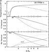Fig. 1. Effect of ion advection on the temperature (top) hydrogen (middle) and helium (bottom) profiles for the case of HD 97658 b. The dashed-dotted lines trace the profiles calculated neglecting the role advection, i.e., by solving the photoionization equilibrium equations in tandem with Euler equations, assuming stationary conditions; the solid lines illustrate how the profiles change when advection is implemented in post-processing, as described in Sect. 2.3. The relatively shallow ionization front in HD 97658 b renders this effect more extreme compared to other planets.

where we substitute the post-processed ionization fraction profiles in the expression of μ and Q, whereas v(r) and ρ(r) are again given by the stationary-state solutions. This enables us to solve for only one unknown, namely T(r) (where the boundary condition is the same as the one adopted for the temporal evolution; see Sect. 5 for details).

We stress that the post-processing scheme described above is only carried out once at the end of each simulation. Overall, this approach yields very good agreement with the ionization and temperature profiles obtained through TPCI (S16), and does so at a fraction of the computing time.

2.4. Two-dimensional effects

Even under the assumption of parallel rays (that is, infinite distance to the star), the geometry of the radiative transfer problem is intrinsically two-dimensional, as the irradiating stellar photons see different optical depths across different atmospheric angles from the substellar point. Moreover, the photo-heating and ionization rates ought to be averaged over the planet day-side (see, e.g., Erkaev et al. 2013).

To simplify this, Odert et al. (2020) modifies the photo-heating rate by dividing the stellar flux by a factor (1 + ατ_E) (Sekiya et al. 1980), arguing that, in the case of HD 189733 b, the solution approximates well the averaged 2D case for α = 4. Instead, S16 adopt the same photo-heating rate as in Eq. (3), and then divide the resulting, steady-state mass loss rate Ṁ = 4πρvr² by a factor of 4, in order to account for the day-side illumination and evaporation. The simulations in this paper are carried out adopting this recipe.

A somewhat different approach – that we propose – stems from the comparison between a tidally-locked planet and a rapidly spinning one. In the former case, the day-side averaged rates will be given by Eqs. (3) and (6) – both divided by a factor of 2 – while the mass outflow originates from one side of the planet, that is Ṁ = 2πρvr². For a rapidly spinning planet, instead, the mass outflow originates from the entire planet, whereas the photo-heating rates will be reduced by a factor of 4 compared to Eqs. (3) and (6) (note, however, that photoevaporation may be negligible for planets far enough from their stars that they could/should be treated as rapidly rotating; for context, a thorough discussion of the two-dimensional effects of irradiation for tidally-locked planets compared to rapidly spinning ones can be found in Showman et al. 2015).

ATES users have the option to select one amongst the above-mentioned recipes. We defer to Sect. 6 for a discussion of the effects of these different approaches to the simulated profiles and mass loss rates.

3. Numerical methods

ATES is a Fortran 90/95 Godunov-type hydrodynamical code that solves the spherical Euler equations numerically, through a finite-volume discretization. ATES has been developed specifically for the study of atmospheric evaporation in exoplanets, although it could be modified for the purpose of simulating more general astrophysical phenomena. The code is built in a modular fashion which allows for the straightforward inclusion (and modification or addition) of different physical processes such as gravity, radiation effects, and chemistry. Its main features are detailed below.

3.1. Spatial grid

The spatial domain extends from R_p, the planetary radius, to R_R, the system Roche lobe radius. It is discretized into N = 500 computational cells. Three different spatial grid types are implemented: a uniform grid, where the grid spacing is Δr_j = (R_R − R_p)/N, which is suitable for problems that do not involve large gradients in the flow parameters close to R_p; a stretched grid, where Δr_j = kΔr_j − 1, $k=R_{\mathrm{R}}^{1/N}$, which is suitable for solutions with moderately high gradients close to R_p; a mixed uniform-stretched grid, where we compute the grid spacing according to

$$\begin{array}{c}\hfill \mathrm{\Delta }{r}_j=\{\begin{array}{c}\begin{array}{cccc}& \mathrm{\Delta }{r}_{\mathrm{low}}=2\times {10}^{-4}{R}_{\mathrm{p}}\hfill & \hfill & \mathrm{if}j<50\hfill \\ \hfill & k\mathrm{\Delta }{r}_{j-1}\hfill & \hfill & \mathrm{if}j\ge 50\hfill \end{array}\hfill \end{array},\end{array}$$(9)

where k is evaluated by solving numerically the following equation through the Newton-Raphson method:

$$\begin{array}{c}\hfill {\displaystyle \frac{1-k^{N-50}}{1-k}}={\displaystyle \frac{R_{\mathrm{R}}-50\mathrm{\Delta }{r}_{\mathrm{low}}}{\mathrm{\Delta }{r}_{\mathrm{low}}}}·\end{array}$$(10)

The last choice is suitable for large gradients close to R_p; this is the default choice in ATES.

3.2. Temporal and spatial discretization

ATES uses the third-order Strong Stability Preserving Runge-Kutta method (SSPRK3; Gottlieb & Shu 1998) for time discretization. We indicate the vectors of cell-averaged conservative variables as U = (ρ, ρv, E)^⊺, while L and S indicate the spatial operators for the hyperbolic and the source terms, respectively. The time integration scheme is written as follows:

$$\begin{array}{c}\hfill \{\begin{array}{c}\begin{array}{cc}& {\mathit{U}}_j^{(1)}={\mathit{U}}_j^n+\mathrm{\Delta }{t}^n({\mathit{L}}_j^n+{\mathit{S}}_j^n)\hfill \\ \hfill & {\mathit{U}}_j^{(2)}=\frac{3}{4}{\mathit{U}}_j^n+\frac{1}{4}{\mathit{U}}_j^{(1)}+\frac{\mathrm{\Delta }{t}^n}{4}({\mathit{L}}_j^{(1)}+{\mathit{S}}_j^{(1)})\hfill \\ \hfill & {\stackrel{\sim }{\mathit{U}}}_j^{n+1}=\frac{1}{3}{\mathit{U}}_j^n+\frac{2}{3}{\mathit{U}}_j^{(2)}+\frac{\mathrm{\Delta }{t}^n}{3}({\mathit{L}}_j^{(2)}+{\mathit{S}}_j^{(2)})\hfill \\ \hfill \end{array}.\hfill \end{array}\end{array}$$(11)

The convective operators are discretized according to the standard, conservative, finite-volume procedure for spherically symmetric flows. In particular, in the jth cell, the components of L are evaluated by the following relations:

$$\begin{array}{c}\hfill {\mathit{L}}_j:=\left(\begin{array}{c}{L}_j^{\rho }\\ L_j^{\rho v}\\ L_j^{\mathrm{E}}\\ \end{array}\right)=-\frac{{\mathcal{A}}_{j+1/2}{\mathit{F}}_{j+1/2}-{\mathcal{A}}_{j-1/2}{\mathit{F}}_{j-1/2}}{\mathrm{\Delta }{\mathcal{V}}_j},\end{array}$$(12)

where F = (ρv, ρv², v(E + p))^⊺ is the flux vector, ${\mathcal{A}}_{j\pm 1/2}=4\pi r_{j\pm 1/2}^2$ is the area of the (j ± 1/2)th cell interface, Δr_j = r_j + 1/2 − r_{j − 1/2} and $\mathrm{\Delta }{\mathcal{V}}_j=4/3\pi (r_{j+1/2}^3-r_{j-1/2}^3)$ are the width and the volume of the jth cell, respectively. The value of the numerical flux at the interfaces is evaluated by a suitable Riemann solver:

$$\begin{array}{c}\hfill {\mathit{F}}_{j\pm 1/2}:=\left(\begin{array}{c}{F}_{j\pm 1/2}^{\rho }\\ F_{j\pm 1/2}^{\rho v}\\ F_{j\pm 1/2}^{\mathrm{E}}\end{array}\right)\approx \mathcal{RP}({\mathit{U}}_{j\pm 1/2}^{\mathrm{L}},{\mathit{U}}_{j\pm 1/2}^{\mathrm{R}}),\end{array}$$(13)

where ${\mathit{U}}_{j\pm 1/2}^{\mathrm{L},\mathrm{R}}$ are the left and right reconstructed states at the interfaces (see Sect. 3.4).

In order to enforce energy conservation, the third component of the flux vector is evaluated as:

$$\begin{array}{c}\hfill F_{j\pm 1/2}^{\mathrm{E}}={[v(E+p)]}_{j\pm 1/2}+F_{j\pm 1/2}^{\rho }{\mathrm{\Phi }}_{j\pm 1/2},\end{array}$$(14)

with Φ_j ± 1/2 ≡ Φ(r_j ± 1/2). The pressure gradient in the momentum equation is included in the source vector, which is evaluated as follows:

$$\begin{array}{c}\hfill {\mathit{S}}_j=\left(\begin{array}{c}0\\ [5pt]-{\displaystyle \frac{{\rho }_{j+1/2}+{\rho }_{j-1/2}}{2}}{\displaystyle \frac{{\mathrm{\Phi }}_{j+1/2}-{\mathrm{\Phi }}_{j-1/2}}{\mathrm{\Delta }{r}_j}}\\ [5pt]{\mathrm{\Phi }}_j{L}_j^{\rho }\end{array}\right)-\left(\begin{array}{c}0\\ {\displaystyle \frac{p_{j+1/2}-p_{j-1/2}}{\mathrm{\Delta }{r}_j}}\\ 0\end{array}\right),\end{array}$$(15)

where ρ_j ± 1/2 and p_j ± 1/2 are evaluated at the cell interfaces.

Radiative contributions to the conservation of energy are integrated in time by performing an explicit Euler step after the hydrodynamical evolution. At each step, the total energy density is updated according to

$$\begin{array}{c}\hfill E^{n+1}={\stackrel{\sim }{E}}^{n+1}+\mathrm{\Delta }{t}^n{Q}^n,\end{array}$$(16)

where Q is the source function defined in Sect. 2.2. The time-step is chosen according to the Courant-Friedrichs-Lewy (CFL) condition (Toro 2009):

$$\begin{array}{c}\hfill \mathrm{\Delta }{t}^n=C_{\mathrm{CFL}}\underset{j}{min}\left(\frac{\mathrm{\Delta }{r}_j}{{|v|}_j^n+c_{\mathrm{s},j}^n}\right)·\end{array}$$(17)

Here, c_s is the local sound speed, and C_CFL = 0.6.

3.3. Approximate Riemann solvers

The flux at the cell interface is computed by means of approximate Riemann solvers. Hereafter, U_L (U_R) will denote the states on the left (right) with respect to the (j + 1/2)th interface.

Three approximate Riemann solvers are implemented into ATES. Firstly, the Harten-Lax-Van Leer with restored contact wave flux (HLLC; Toro et al. 1994), which is based on a three-wave model for the structure of the exact solution of the Riemann problem. The HLLC flux is given by

$$\begin{array}{c}\hfill {\mathit{F}}_{j+1/2}=\{\begin{array}{c}\begin{array}{cccc}& {\mathit{F}}_{\mathrm{L}}\hfill & \hfill & 0\le S_{\mathrm{L}}\hfill \\ \hfill & {\mathit{F}}_{\ast \mathrm{L}}\hfill & \hfill & S_{\mathrm{L}}\le 0\le S_{\ast }\hfill \\ \hfill & {\mathit{F}}_{\ast \mathrm{R}}\hfill & \hfill & S_{\ast }\le 0\le S_{\mathrm{R}}\hfill \\ \hfill & {\mathit{F}}_{\mathrm{R}}\hfill & \hfill & 0\ge S_{\mathrm{R}}\hfill \\ \hfill \end{array},\hfill \end{array}\end{array}$$(18)

where F_*K = F_K + S_K(U_*K − U_K), with K = L, R, and

$$\begin{array}{c}\hfill {\mathit{U}}_{\ast K}={\rho }_K\left(\frac{S_K-v_K}{S_K-S_{\ast }}\right)\left(\begin{array}{c}1\\ S_{\ast }\\ {\displaystyle \frac{E_K}{{\rho }_K}}+(S_{\ast }-v_K)[S_{\ast }+{\displaystyle \frac{p_K}{{\rho }_K(S_K-v_K)}}]\\ \end{array}\right).\end{array}$$(19)

The three characteristic speeds are chosen from Batten et al. (1997);

$$\begin{array}{c}\hfill \begin{array}{cc}& S_{\mathrm{L}}=min(0,v_{\mathrm{L}}-c_{\mathrm{sL}},v_{\mathrm{R}}-c_{\mathrm{sR}})\hfill \\ \hfill & S_{\mathrm{R}}=min(0,v_{\mathrm{L}}+c_{\mathrm{sL}},v_{\mathrm{R}}+c_{\mathrm{sR}})\hfill \\ \hfill & S_{\ast }=\frac{p_{\mathrm{R}}-p_{\mathrm{L}}+{\rho }_{\mathrm{L}}{v}_{\mathrm{L}}(S_{\mathrm{L}}-v_{\mathrm{L}})-{\rho }_{\mathrm{R}}{v}_{\mathrm{R}}(S_{\mathrm{R}}-v_{\mathrm{R}})}{{\rho }_{\mathrm{L}}(S_{\mathrm{L}}-v_{\mathrm{L}})-{\rho }_{\mathrm{R}}(S_{\mathrm{R}}-v_{\mathrm{R}})}·\hfill \end{array}\end{array}$$(20)

This scheme is able to handle solutions containing both smooth regions as well as discontinuities which may arise during the temporal evolution; this is the default choice in ATES.

Secondly, the Roe solver (Roe 1981), which is based on the exact solution of a local linearized Riemann problem at the interface. In this case, the flux is given by:

$$\begin{array}{c}\hfill {\mathit{F}}_{j+1/2}=\frac{1}{2}({\mathit{F}}_{\mathrm{L}}+{\mathit{F}}_{\mathrm{R}})-\frac{1}{2}{\displaystyle \sum _{i=1}^3{\stackrel{\sim }{\alpha }}_i|{\stackrel{\sim }{\lambda }}_i|{\stackrel{\sim }{\mathit{K}}}^{(i)},}\end{array}$$(21)

where the wave strengths ${\stackrel{\sim }{\alpha }}_i$, the eigenvalues ${\stackrel{\sim }{\lambda }}_i$ and the eigenvectors ${\stackrel{\sim }{\mathit{K}}}^{(i)}$ of the Jacobian are evaluated on a reference state defined from averages (e.g., Toro 2009):

$$\begin{array}{c}\hfill \left(\begin{array}{c}\stackrel{\sim }{\rho }\\ \stackrel{\sim }{v}\\ \stackrel{\sim }{H}\end{array}\right)=\left(\begin{array}{c}\sqrt{{\rho }_{\mathrm{L}}{\rho }_{\mathrm{R}}}\\ {\displaystyle \frac{\sqrt{{\rho }_{\mathrm{L}}}{v}_{\mathrm{L}}+\sqrt{{\rho }_{\mathrm{R}}}{v}_{\mathrm{R}}}{\sqrt{{\rho }_{\mathrm{L}}}+\sqrt{{\rho }_{\mathrm{R}}}}}\\ {\displaystyle \frac{\sqrt{{\rho }_{\mathrm{L}}}{H}_{\mathrm{L}}+\sqrt{{\rho }_{\mathrm{R}}}{H}_{\mathrm{R}}}{\sqrt{{\rho }_{\mathrm{L}}}+\sqrt{{\rho }_{\mathrm{R}}}}}\end{array}\right)·\end{array}$$(22)

Here H = (E + p)/ρ is the specific entalpy of the gas. The code includes also the Harten-Hyman entropy. This option is suitable for those cases where possible discontinuities ought to be resolved with high accuracy.

Lastly, the Local Lax-Friedrichs flux (LLF; Rusanov 1962), in which the numerical flux is evaluated as

$$\begin{array}{c}\hfill {\mathit{F}}_{j+1/2}=\frac{{\mathit{F}}_{\mathrm{L}}+{\mathit{F}}_{\mathrm{R}}}{2}-{\alpha }_{j+1/2}({\mathit{U}}_{\mathrm{R}}-{\mathit{U}}_{\mathrm{L}}),\end{array}$$(23)

where α_j + 1/2 = max(|v_L|+c_sL, |v_R|+c_sR) is the maximum local eigenvalue of the Jacobian of the Euler’s equations (Eq. (1)). The LLF solver is the least computationally expensive option; however, it is also the most diffusive, and thus should be used only in conjunction with a high resolution reconstruction scheme (see Sect. 3.4).

3.4. Reconstruction

The accuracy of the reconstruction of the left and right states at a given interface determines the overall spatial accuracy of the numerical scheme. Within ATES, the reconstruction is carried out in primitive variables W = (ρ, v, p)^⊺.

Two reconstruction schemes are available to the user, with second and third order accuarcy, respectively.

In the second-order Piecewise Linear reconstruction Method (PLM; see, e.g., LeVeque 2002), the states at the interfaces of the jth cell are reconstructed through a linear interpolation on the stencils {j − 1, j} and {j, j + 1}:

$$\begin{array}{c}\hfill \{\begin{array}{c}\begin{array}{cc}\hfill {\mathit{W}}_{\mathrm{R},j-1/2}& ={\mathit{W}}_j-\frac{1}{2}\sigma \mathrm{\Delta }{r}_{j-1/2}\hfill \\ \hfill {\mathit{W}}_{\mathrm{L},j+1/2}& ={\mathit{W}}_j+\frac{1}{2}\sigma \mathrm{\Delta }{r}_{j+1/2}\hfill \end{array},\hfill \end{array}\end{array}$$(24)

where σ is a limited slope evaluated through the generalized MINMOD limiter (Kurganov & Tadmor 2000) with θ = 2,

$$\begin{array}{c}\hfill \sigma =\mathrm{M}\text{IN}\mathrm{M}\text{OD}(\theta {\displaystyle \frac{\mathrm{\Delta }{\mathit{W}}_{j+1/2}}{\mathrm{\Delta }{r}_{j+1/2}}},\theta {\displaystyle \frac{\mathrm{\Delta }{\mathit{W}}_{j-1/2}}{\mathrm{\Delta }{r}_{j-1/2}}},{\displaystyle \frac{\mathrm{\Delta }{\mathit{W}}_{j+1/2}+\mathrm{\Delta }{\mathit{W}}_{j-1/2}}{\mathrm{\Delta }{r}_{j+1/2}+\mathrm{\Delta }{r}_{j-1/2}}})·\end{array}$$(25)

The MINMOD function is defined as

$$\begin{array}{c}\hfill \mathrm{M}\text{IN}\mathrm{M}\text{OD}(x_1,x_2,\dots )=\{\begin{array}{c}\begin{array}{cc}\hfill \underset{j}{min}\{x_j\}& \mathrm{if}{x}_j>0\forall j\hfill \\ \hfill \underset{j}{max}\{x_j\}& \mathrm{if}{x}_j<0\forall j\hfill \\ \hfill 0& \mathrm{otherwise}.\hfill \end{array}\hfill \end{array}\end{array}$$(26)

Conversely, the third order, Energy Stable Weighted Essentially Non-Oscillatory scheme (ESWENO3; Yamaleev & Carpenter 2009; Mignone et al. 2012) employs a weighted convex combination of second-order interpolants to produce a third-order parabolic reconstruction of the left and right states. Here, we follow the compact formulation of Mignone et al. (2012). In the jth cell, the reconstructed states are evaluated as follows:

$$\begin{array}{c}\hfill \{\begin{array}{c}\begin{array}{cc}\hfill {\mathit{W}}_{\mathrm{L},j+1/2}& ={\mathit{W}}_j+\frac{1}{2}{\displaystyle \frac{2a_{+}\mathrm{\Delta }{\mathit{W}}_{j+1/2}+a_{-}\mathrm{\Delta }{\mathit{W}}_{j-1/2}}{2a_{+}+a_{-}}}\hfill \\ \hfill {\mathit{W}}_{\mathrm{R},j-1/2}& ={\mathit{W}}_j-\frac{1}{2}{\displaystyle \frac{a_{+}\mathrm{\Delta }{\mathit{W}}_{j+1/2}+2a_{-}\mathrm{\Delta }{\mathit{W}}_{j-1/2}}{a_{+}+2a_{-}}}\hfill \\ \hfill \end{array}.\hfill \end{array}\end{array}$$(27)

The coefficients a_± are the weights proposed by Yamaleev & Carpenter (2009):

$$\begin{array}{c}\hfill a_{\pm }=1+\frac{{(\mathrm{\Delta }{\mathit{W}}_{j+1/2}-\mathrm{\Delta }{\mathit{W}}_{j-1/2})}^2}{{\left(\mathrm{\Delta }{r}_j\right)}^2+{\left(\mathrm{\Delta }{\mathit{W}}_{j\pm 1/2}\right)}^2}·\end{array}$$(28)

Both methods were used in turn; the PLM reconstruction method was employed first, starting from the initial conditions described below (Sect. 5). Once fractional variations in the mass flux had reached a reference value of ΔṀ/Ṁ ≲ 0.5 − 1, the simulation was interrupted. The output profiles were specified as initial conditions for the second part of the run, which employed the ESWENO3 reconstruction method. The simulation was stopped when the mass outflow reached steady-state, with tolerance set to ΔṀ/Ṁ < 0.001.

3.5. Ionization equilibrium

At each time-step, the simplified photoionization equilibrium equations (Eq. (5) with the l.h.s. advection terms set equal to 0) are solved through a modification of the Powell dogleg method (Powell 1970), available through the MINPACK library². The differential Eqs. (7) and (8) are solved by means of a standard, implicit Euler method, under the assumptions discussed in Sect. 2.2.

4. Code validation

Here we present two standard problems that are routinely used to validate the performance of radiation hydrodynamics numerical schemes. Specifically, we test the pure hydrodynamical discretization and the photoionization equilibrium modules separately, by modeling the classical Sedov blast wave and the rarefied ionization fronts problems.

4.1. Sedov blast wave

In this classical test, a certain amount of energy is suddenly released in a small region of a low-density gas, initially assumed at rest. Sedov (1959) derived the homonymous, self-similar solution of the Euler equations for this problem, which describes the formation and propagation of a blast wave. This test is especially useful for validating ATES’ ability to deal with strong discontinuities in spherical coordinates. On a uniform grid of 500 cells extending in the (dimensionless) space range [0, 1/2], we start from a (dimensionless) initial constant density ρ = 1 and pressure p = 10⁻⁵. A total energy E = 1 is deposited into the first computational cell at r = 0. Euler equations are then solved for an elapsed time t = 0.05, adopting reflective boundary conditions at r = 0 and free-flow conditions at the upper boundary of the domain. The resulting density, velocity and pressure of the blast wave, shown as black crosses in Fig. 2, are all in excellent agreement with the exact solutions, shown as blue lines.

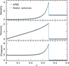Fig. 2. Sedov blast wave solution at t = 0.05; the solid blue lines correspond to the exact solutions of the Euler equations, while the black crosses are the numerical values obtained by ATES employing the ESWENO3 reconstruction method and the HLLC approximate Riemann solver.

4.2. Rarefied ionization front

As a second test, we simulate the formation of an H II region around a central ionizing source. This is meant to validate the implementation of the numerical solver for the photoionization equilibrium equations.

A hot (O-type) star, with a T_⋆ = 50 000 K blackbody spectrum, is placed at the origin of the reference system. A neutral, homogeneous hydrogen nebula with constant density n_H = 10⁴ cm⁻³ fills the domain, which extends up to 0.3 pc. The nebula is initially at rest, at a temperature of T = 100 K. A strong shock wave develops as soon as the central source is switched on. The position of the R-type Ionization Front (IF) follows the well-known result of Strömgren (1939):

$$\begin{array}{c}\hfill R_{\mathrm{IF}}(t)=R_{\mathrm{S}}{(1-e^{-t/t_{\mathrm{rec}}})}^{1/3},\end{array}$$(29)

where t_rec = (α_rec,H IIn_e)⁻¹ is the case-B recombination time for H II, and the so-called Strömgren radius for an isothermal sphere is found by balancing the total number of recombinations and photoionizations:

$$R_{\mathrm{S}}={\left(\frac{3\dot{N}}{4\pi n_{ \text{H} \text{I}}^2{\alpha }_{\mathrm{r}\mathrm{e}\mathrm{c}, \text{H} \text{II}}(T)}\right)}^{1/3}\cdot$$(30)

Here, Ṅ is the number of ionizing photons emitted per second by the star. For a stellar radius of 10 R_⊙, we found Ṅ ≃ 3.8 × 10⁴⁹ s⁻¹. Assuming a gas temperature of T = 2.2 × 10⁴ K, we found α_rec,H II ≃ 1.31 × 10⁻¹³ cm³ s⁻¹. The inferred Strömgren radius is then R_S ≃ 0.29 pc.

We adopted a radial grid of N = 1000 points, with zero-gradient boundary conditions on all variables. The solution has been advanced in time up to 5 t_rec. The post-processing routine described in Sect. 2 (to account for advection) has not been used here. The time-step is limited by the minimum recombination time value in the domain, $\mathrm{\Delta }{t}_{\mathrm{rec}}^n={[max(n_{\mathrm{e}}^n{\alpha }_{\mathrm{rec},\mathrm{H}\mathrm{I}\mathrm{I}}(T^n))]}^{-1}$, and by ensuring the positivity of the internal energy, $\mathrm{\Delta }{t}_{\text{rad}}^n=0.9\text{min}(E^n/|Q^n|)$. We thus chose $\mathrm{\Delta }{t}^n=\text{min}(\mathrm{\Delta }{t}_{\text{rec}}^n,\mathrm{\Delta }{t}_{\text{rad}}^n)$.

As shown in the top panel of Fig. 3, the numerical IF (black crosses) propagates at a faster pace compared to the analytical solution (blue line) during the early stages of the evolution. During this phase, the temperature of the H II region is significantly lower than the final equilibrium temperature, and the resulting recombination timescale is longer than the radiative timescale, that is, ionization and recombination are out of equilibrium. As ATES computes the ionization fractions under an assumed equilibrium, the IF velocity is necessarily overestimated for t ≪ t_rec, when in fact equilibrium is actually not settled. It is only at later times, when the temperature reaches ∼10⁴ K, as indicated by the solid line in the lower panel of Fig. 3, that the recombination and radiative timescales become comparable, and thus the asymptotic value of the IF position evaluated by ATES matches the Strömgren radius.

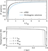Fig. 3. Results from the simulation of the temporal evolution of a rarefied ionization front. Top panel: temporal evolution of the ionization front. The evolution of the ionization front position (in units of RS; see Eq. (30)) computed by ATES is represented by the black crosses, and compared to the analytical solution (see Eq. (29)), shown by the solid blue line. Bottom panel: the ionization front temperature profiles are shown at different times, as a function of the distance from the central star.

5. Simulation setup

In order to run ATES for a specific exoplanet, Euler’s equations (Eq. (1)) were recast in dimensionless form, with the planet radius R_p serving as unit length and $\sqrt{k_{\mathrm{B}}{T}_{\mathrm{p}}/m_{\mathrm{H}}}$ as unit velocity, T_p being the gas temperature at the planet radius (the so-called planet equilibrium temperature with zero albedo).

The planet atmosphere was then initialized as a fully neutral, isothermal sphere composed by H and He (with number ratio set to the cosmological value of 1/12 in the cases presented here), with a liner initial velocity profile: v(t = 0) = (r − 1)/2. The atmospheric density and temperature at the planet radius were chosen according to realistic physical conditions. The total number density at planet radius was set to 10¹⁴ cm⁻³, the same value adopted by S16. The reader is referred to their Sect. 3.6 for a detailed discussion of the effects the chosen value has on the stationary solutions. The equilibrium temperature depends on the specific planet. For the runs describe in next Sect. 6, again we adopted the same values as S16 (see their Table 1 for references). The value of the velocity in the ghost cells at the lower boundary was obtained through a zero-th order extrapolation from the first computational cell in the case of inflow characteristics, while it was set to zero otherwise. At the upper boundary (that is, at the Roche lobe radius), a zero-gradient condition is applied to all quantities if the PLM reconstruction method is employed; in the case of the ESWENO3 reconstruction, the ghost cells were filled with linearly extrapolated values from the outermost cell of the domain.

The stellar spectrum was modeled as a piece-wise power-law with the specific flux ∝E⁻¹, both in the EUV band ([13.6, 124] eV), and the X-ray band ([0.124, 12.4] keV). The spectrum in each band is normalized to the EUV and X-ray luminosities reported by S16 for each planet. The validity of this approximation is discussed in Sect. 6.

All the simulations presented in this work were performed employing: the mixed uniform-stretched grid, the HLLC approximate Riemann solver and the PLM reconstruction scheme – followed by ESWENO reconstruction scheme (see Sect. 3 above for details). A typical simulation run for a few tens of minutes on a 2.7 GHz quad-core CPU, with some cases taking as little as a few minutes, up to a few hours for the most time-consuming cases. By comparison, S16 reports that “The computational effort of the presented simulations corresponds approximately to 300 000 h on a standard 1 GHz CPU”; this refers to all of the 18 planets listed in their Table 1.

6. Results and discussion

A thorough discussion of the properties of the simulated atmospheres on a case-by-case basis can also be found in S16; here, we focus on presenting the results of our numerical simulations vis-à-vis those obtained by S16 with TPCI (Salz et al. 2015). Specifically, S16 focus on a sample of 18 nearby (within 120 pc) planets, selected a priori on the basis of the expected detectability of their out-flowing atmospheres through Lyα transit spectroscopy; 14 out of those are actually found by TPCI to have non-negligible outflow rates³. For comparison purposes, we run ATES on the same 14 systems, adopting the same planetary and stellar parameters (listed in Table 1), with the only notable difference that, whereas S16 estimate the SED of the host stars using a complex piece-wise reconstruction method (see Sect. 2.2 of S16), we take their estimated X-ray and EUV luminosities at face value, and use them to normalize a ∝E⁻¹ spectrum in either bands (noting that the stellar SEDs in Fig. 1 of S16 are roughly consistent with flat spectra in νF_ν).

This simplification is motivated by the following reasoning. In the first approximation, the problem of atmospheric photo-heating can be thought of as an inverse Strömgren sphere. As for the textbook case, where one only distinguishes between fully neutral and fully ionized regions, the location and velocity of the ionization front depend only on the rate of photons with energies above a given element ionization threshold. This is true even for the more realistic case when the photon rate is weighted over the appropriate (frequency-dependent) cross sections. Thus, as long as the underlying spectral shape and normalization preserve the total number of photons per unit time in each band, the properties of the ionization front are fairly insensitive to small features in the stellar SED.

Ultimately, our approach is validated by the remarkably good agreement between the outflow parameters estimated by ATES and those obtained by TPCI. The density, velocity, temperature, pressure and ionization profiles obtained from both codes are shown in Figs. 4–6 for three case studies: HD 97658 b (low gravity, low irradiation), WASP-80 b (moderate gravity, moderate irradiation), and WASP-43 b (high gravity, high irradiation), respectively.

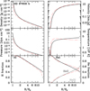Fig. 4. Simulated density, velocity, pressure, temperature, neutral hydrogen (H I), neutral helium (He I), single-ionized helium (He II), and double ionized helium (He III) fractions, for the case of HD 97658 b. The thick solid black lines trace the profiles as calculated by ATES, to be compared to those obtained by TPCI (S16), shown as dashed red lines. We note that the He III curves in the bottom right panel practically overlap.

Fig. 5. Same as for Fig. 4, but for WASP-80 b.

Fig. 6. Same as for Fig. 4, but for WASP-43 b.

As noted by S16, the simulated atmospheres have qualitatively similar structures; the temperature profiles exhibit a very sharp rise starting from the height where the bulk of the stellar radiation is absorbed. This happens right at the planet radius for the case of WASP-80 b and WASP-43 b, whereas the temperature begins to rise sharply at ≃1.1 R_p in the case of HD 97658 b, which has a higher atmospheric density. The steep temperature gradient of the lower atmosphere is responsible for driving the atmospheric expansion against the gravitational pull of the planet. The temperature profiles all reach a maximum value further out, where the net cooling rate starts to decrease (see below). Mass outflows are initially very slow, with inferred velocities of a few cm s⁻¹ at the inner boundary, and reach supersonic velocities at the Roche lobe height, with steady-state values between 10 and 20 km s⁻¹.

In general, sharp ionization fronts are typical of highly irradiated planets (such as WASP-43 b), whereas more gradual temperature profiles are typical of less irradiated planets with shallow ionization fronts. The structure and composition of the atmosphere depend on the strength of the stellar irradiation: WASP-43 b, with an incident EUV flux log F_EUV = 4.82 (in cgs units, close to 10 000 the solar irradiance at Earth in the same band; see, e.g., Ribas et al. 2005), exhibits a very sharp hydrogen ionization front (Fig. 6, lower panels). A thin layer of neutral hydrogen (H I) is confined within less than 1.3 planetary radii, above which hydrogen is fully ionized (the H I fraction is < 10% at 1.2 R_p). Unsurprisingly, the neutral helium profile (He I) tracks that of H I, whereas the percentage of double-ionized helium (He III), which is higher than 90% beyond 2 R_p, starts to drop below this height, and reaches 10% at 1.2 R_p, where the He II fraction peaks (reaching ≃80%). By comparison, HD 97658 b experiences a factor 70 lower stellar irradiation compared to WASP-43 b; its ionization front is very shallow (Fig. 4); the H I fraction declines gently, from 100% at R_p to ∼40% at the Roche height; the He I profile mirrors H I’s qualitatively, whereas the percentage of He II increases from close to zero at the inner boundary to about 40% at the Roche height, with He III never reaching above a few per cent. The ionization profiles of WASP-80 b–whose stellar irradiance is a factor 6 lower than WASP-80 b, and a factor 11 higher than HD 97658 b–are qualitatively intermediate (see Fig. 5).

The outflow behavior can be better understood by examining the contributions to the atmospheric heating and cooling from different mechanisms; these are shown in Figs. 7–9 for the same three planets discussed above. The stellar photo-heating rate is represented by the solid, thick red line; the radiative cooling term, represented by the thick, solid blue line, is given by the sum of all the possible contributions: collisional excitation (Lyα), bremsstrahlung, recombinations and collisional ionization (shown with different line styles and shades of blue); adiabatic cooling is represented by the solid thick green line, whereas advective cooling and heating are shown as solid purple and orange lines, respectively. For comparison, the radiative heating and cooling terms from TPCI are shown as light and dark gray lines, respectively. The most notable difference in the heating and cooling rates amongst the three planets has to do with the relative importance of radiative vs. adiabatic cooling. Whereas the latter completely dominates over the former across the entire domain for HD 97658 b, the situation is nearly reversed for the high-gravity and high-irradiation planet WASP-43 b, where radiative (and primarily Lyα) cooling within ≲1.5 R_p exceeds adiabatic cooling by up to 2 orders of magnitude; further out, the high ionization fraction makes radiative cooling inefficient. Once again, the behavior of WASP-80 b is intermediate between HD 97658 b and WASP-43 b, in that radiative cooling here exceeds adiabatic cooling in the inner regions, albeit not as strikingly as in the case of WASP-43 b.

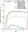Fig. 7. Simulated specific heating and cooling rate profiles for the atmosphere of HD 97658 b, broken into individual, contributing mechanism (see legend for details); the dark and light gray curves, respectively, trace the photo-heating and cooling rates obtained by TPCI (S16). In the case of the low-gravity, low-irradiation planet HD 97658 b, atmospheric escape is driven by adiabatic expansion, with negligible contribution from radiative cooling.

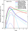Fig. 8. Same as for Fig. 7, but for WASP-80 b. In the case of this moderate-gravity, moderate-irradiation planet, atmospheric escape is mainly driven by radiative cooling in the innermost region, albeit with a non-negligible contribution from adiabatic expansion; further out, where the ionization fraction approaches 100%, adiabatic expansion takes over and dominates the cooling.

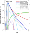Fig. 9. Same as for Fig. 7, but for WASP-43 b. In the case of this high-gravity, high-irradiation planet, atmospheric escape is entirely driven by radiative cooling in the innermost region; only further out, where the ionization fraction approaches 100%, adiabatic expansion takes over and dominates the cooling.

Last, in Fig. 10 we compare the steady-state mass outflows estimated by ATES (in black) vs. TPCI (in red). Overall, the agreement is very good, to within a factor of 2, which is arguably lower than the “systematic” uncertainties associated with the modeling (see Sect. 3.2 in S16 for quantitative estimates). Whenever they differ, the ATES mass outflow rates tend to be higher than TPCI’s. A close inspection of the outflow properties suggests that this difference is rooted in the density profiles, as ATES’ are slightly higher than TPCI’s (this is true for all the simulated systems). Although the impact on the resulting mass outflow rates is modulated by the velocity profiles, for which we find no systematic trend, higher density profiles are bound to yield higher steady-state mass outflow rates. Considering that ATES employs the same boundary conditions as TPCI at the planet radius, the higher densities are likely to arise from the fact that ATES implements ion advection in post-processing (Sect. 2) as opposed to at each time-step. In fact, ion advection has the effect to alter (ever so slightly) the atmospheric density at each time-step; in turn, this yields slightly different heating rates, and thus dynamical evolution. By accounting for the effects of advection in post-processing, ATES is likely to underestimate such time-integrated advection effects. At the same time, it is important to stress that doing so massively reduces the computational time whilst recovering realistic ionization fraction profiles (see Fig. 1).

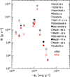Fig. 10. Simulated, steady-state mass outflow rates from the 14 planetary systems considered in this work. The values obtained by ATES (in black) are compared to those by TPCI (S16, in red). Overall, the estimated mass loss rates agree to within a factor of 2 in all cases. In those cases where ATES differs from TPCI, the differences are always upward, and are likely due to inclusion of ion advection, which ATES implements in post-processing, yielding systematically higher atmospheric density profiles. This implementation choice, however, is chiefly responsible for the dramatic gain in computational time.

As stated in Sect. 2.1, ATES does not include any molecular forms of hydrogen. According to Odert et al. (2020), the role of H molecules is likely to be significant only for cool(er) atmospheres, very close to the planet radius, at ≲1.1 R_p. More specifically, the main molecular coolant in H₂ dominated atmospheres is IR radiation from ${\text{H}}_3^{+}$; such cooling is expected to be negligible at small orbital distances or high EUV fluxes (Koskinen et al. 2007; Shaikhislamov et al. 2014; Chadney et al. 2015; however, see, e.g., Shematovich 2010 for the role of H₂ dissociation in producing supra-thermal H atoms). Whereas we do not expect that the omission of H molecules has any significant impact on the results presented here, that is, for moderately and highly irradiated planets (F_XUV ≳ 10² − 10³ in cgs units), we plan to include molecular hydrogen in the next release of the code.

We now turn our attention to the treatment of 2D effects. As discussed in Sect. 2.4, different methods are employed in the literature to account for the fact that the photoionizing photons see different optical depths through the atmosphere, as well as averaging the photo-heating rate over the planet day-side. In order to allow for a proper comparison with TPCI, the simulations presented here were run by adopting the same prescription as S16, that is, by diving the output mass loss rate by 4 (method (i)). In order to illustrate the effects of different choices, we re-run ATES using (ii) the prescription by Odert et al. (2020), as well as (iii) dividing the photo-heating by a factor 4 (which we suggest would be appropriate for the case of a rotating planet), and (iv) dividing both the photo-heating rate and the output mass outflow rate by 2 (appropriate for the case of a a tidally locked planet).

For the case of GJ 3470 b, the resulting mass outflow rates differ by a factor 2 at most; specifically, we obtain log Ṁ = 10.76 using method (i), vs. 10.66 actually reported by S16. By comparison, method (ii) yields log Ṁ = 10.93; method (iii) yields log Ṁ = 10.81, whereas method (iv) yields log Ṁ = 10.86. We expect that the magnitude of the difference will be greater for planets where the atmospheric cooling is dominated by radiative (as opposed to adiabatic) cooling; in this respect, GJ 3470 b can be thought of as an intermediate case, where both cooling channels contribute equally. We verified that this is indeed the case by carrying out the same set of simulations for the highly irradiated gas giant WASP-77 A b; in this case, the resulting mass outflow rates obtained by ATES are log Ṁ = 9.07, 9.52, 8.88, 8.98 for method (i), (ii), (iii) and (iv), respectively, that is a factor ∼4 difference at most. We caution, however, that the highest Ṁ results from dividing the stellar flux by a factor (1 + ατ_E), with α = 4 (Odert et al. 2020). This choice of α is meant to approximate the averaged 2D case in the specific case of HD 189733 b, and it is thus not obvious whether it can be extended to the case of a planet which is likely to have a more extended atmosphere.

6.1. ATES: Applicability and numerical limitations

ATES’ range of applicability and validity is bounded by two classes of limitations: physical and numerical. The former include the 1D approximation, the lack of H molecules, and neglecting ion-ion interactions, conductivity and the mixing of different species. The effects and implications of these approximations are discussed at various points throughout the paper. Here, we focus on the latter; specifically, we aim to define ATES’ range of applicability by performing a numerical convergence analysis on a physically relevant, bounded subspace of the F_XUV − Φ_p parameter space (planetary stellar flux and gravitational energy, respectively). Having demonstrated that ATES yields good agreement with the same planets for which S16 are able to obtain steady-state mass outflows, we test the code under more extreme choices of input parameters, such as extremely irradiated atmospheres and quasi-stable atmospheres (that can be expected for gas giants that experience moderate to low irradiation).

To this end, we start with simulating a handful of additional, well-known systems: five low-mass planets whose atmospheres are expected to be undergoing “boil-off” (Owen & Wu 2016), namely: CoRoT-24 b, Kepler-36 b,c, and Kepler-11 b,c (see, e.g., Lammer et al. 2016; Owen & Morton 2016; Cubillos et al. 2017)⁴. To those we add new simulations for a handful of moderately-irradiated gas giants whose atmospheres are likely not undergoing hydro-dynamical escape, namely: WASP-38 b, WASP-8 b, WASP-10 b, WASP-18 b, HAT-P-2 b, and HAT-P-20 b; both stellar and planetary parameters for these systems were taken from S16 and references therein. The results of this investigation are summarized in Fig. 11. Those systems for which ATES reaches or fails to reach convergence are represented as filled and open circles, respectively. For the former group, decreasing values of mass outflow rates are characterized by progressively cooler colors. In general, we observe a trend whereby the code fails to reach convergence for the heaviest gas giants. The lack of known gas giants experiencing low irradiation (namely, with log(−Φ_p)≳13 and log F_XUV ≲ 3, in cgs units) prevents us from characterizing any possible dependence of the convergence on irradiation, although the very fact that the solution convergence is reached for CoRoT-2 b and not for WASP-8 b (which have comparable Φ_p) suggests that irradiation does indeed play a role. To fully parse ATES’ range of applicability, we further simulate a large set of mock planets, sampling the gravity-stellar flux plane at higher resolution. This enables us to define a quantitative criterion for convergence, which is illustrated by the dashed line in Fig. 11: log(−Φ_p)≲12.9 + 0.17 log F_XUV (cgs units). Below this approximate threshold, ATES can be reliably expected to reach convergence and yield a steady-state atmospheric mass outflow rate. Conversely, systems above this threshold were all identified by S16 as likely undergoing Jeans escape.

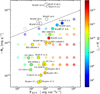Fig. 11. All the planetary systems simulated in this study are shown in the (Φp, FXUV) plane, and color-coded based on the estimated mass loss rate illustrated by the right-hand side bar. Open, color-less circles show those cases for which ATES fails to converge. In general, known planets are identified by their names and highlighted by a circle; all the others are “synthetic”. ATES recovers stable, steady-state solutions for systems with log(−Φp)≲12.9 + 0.17 log FXUV (in cgs units); such convergence threshold is marked by the dashed black line.

6.2. Comparison to other existing codes

Beside TPCI (Salz et al. 2015), which we used as a benchmark for our simulations, several other codes exist in the literature which are used to model atmospheric escape in exoplanets. Generally speaking, they can be divided in two categories: dedicated, proprietary hydrodynamic-radiative codes (mostly 1D), and public, multipurpose 3D codes, or adaptations thereof (such as TPCI, Salz et al. 2015). We note that we are intentionally limiting the discussion below to numerical works that were developed over the last 5 years, thus omitting early, seminal works.

Notable amongst the former is the 1D code developed by Erkaev et al. (2016); similar to ATES in its hydrodynamics, energy and ionization balance treatment (unlike ATES, it includes thermal conduction, but neglects He), this code has been extensively used (by the many contributing authors) to estimate the atmospheric profiles and mass outflow rates for several, well-known, highly irradiated exoplanets (e.g., Erkaev et al. 2017; Fossati et al. 2017; Kubyshkina et al. 2018a; Odert et al. 2020, to name a few). More recently developed (proprietary) 1D hydrodynamics codes include Vidotto & Cleary (2020) (following Allan & Vidotto 2019), which computes the effects of the stellar wind ram pressure on the atmospheric outflow, and Bisikalo et al. (2018), which adapts the code by (Ionov et al. 2017) to account for the role of supra-thermal photo-electrons during stellar flares. Somewhat separately, Chen & Rogers (2016) developed a prescription to adapt the capabilities of the Modules for Experiments in Stellar Astrophysics (MESA) to model sub-Neptune-sized planets with H-He envelopes. This planetary evolution module, along with subsequent variations and/or improvements, has been widely used to ascertain the role of thermal evolution vs. stellar irradiation in shaping the observed distribution of exoplanet radii (Fulton et al. 2017). As an example, Kubyshkina et al. (2020) and Kubyshkina & Fossati (2021) study the evolution of planetary atmospheres under the combined effects of atmospheric mass loss (modeled using the proprietary code by Kubyshkina et al. 2018a) and planetary thermal evolution (modeled using MESA, after Paxton et al. 2019). A separate mention goes to Koskinen et al. (2014) and Khodachenko et al. (2019), and references therein, who performed detailed 3D hydrodynamic simulations of a handful of giant planets with proprietary codes that feature extensive chemical networks.

Turning to publicly available, multipurpose codes, Debrecht et al. (2019) carry out 3D simulations of atmospheric outflows from synthetic planets with ASTROBEAR, a parallelized, magneto-hydrodymamics (MHD) code designed for 2D and 3D adaptive mesh refinement simulations. The same code is used by Debrecht et al. (2020) to investigate the role of the stellar Lyα radiation pressure on the outflow dynamics. In these studies ASTROBEAR is set up to simulate a single frequency, planar radiation field impacting on a primordial, atomic H atmosphere. Along the same lines, McCann et al. (2019) adopt the 3D, MHD Eulerian code ATHENA (Stone et al. 2008), complemented by dedicated ionization and radiative transfer modules, to simulate planetary atmospheres, also including the stellar wind and Coriolis force effects. A similar approach is that by Esquivel et al. (2019) who adapt the publicly available 3D MHD code GUACHO (Esquivel et al. 2009) to investigate the interaction between the stellar and planetary winds, also accounting for radiation pressure and charge exchange.

The latter type of studies are typically focused on a specific planetary system with a wealth of available data, where employing a sophisticated 3D code allows for a detailed (if time-consuming) morphological characterization of the outflow, including, for example, the possible development of cometary tails. In contrast, 1D codes that allow for a swift estimate of the outflow properties, including the instantaneous mass-outflow rate, can be thought of as an efficient tool for assessing the most promising targets for intensive spectroscopic follow-ups out of a large pool of systems. Amongst these, ATES has the added benefit of being fast – a typical run takes minutes-to-hours on a standard laptop to achieve convergence – and publicly available.

7. Conclusions

In summary, we have developed a new and efficient photoionization hydrodynamics code that can be easily employed to readily estimate the instantaneous atmospheric mass loss rates from highly irradiated planets. The code, which is publicly available, can be run through an intuitive graphic interface where the user can specify the grid and reconstruction method of choice. For a given choice of planetary and stellar parameters, the code calculates the corresponding atmospheric temperature, density, velocity and ionization fraction profiles, for a primordial composition of atomic H and He, where the (user-specified) H-to-He ratio is kept fixed throughout the simulation.

The ATES results are in very good agreement with those obtained by TPCI (The Pluto Cloudy Interface; S16) for 14 moderately-to-highly irradiated systems (see Table A.2 and Fig. 10); minor differences are likely due to the implementation of ion advection, which ATES carries out in post-processing (Sect. 2.3). This scheme, however, results in a major speed-up in calculation, with the considered 14 systems taking between 3 min to up to 2 h (depending on the actual case) on a standard 2.7 GHz quad core CPU.

A comprehensive description of the code installation and usage is also available as part of the online repository. Future developments will involve the inclusion of molecular hydrogen as well as metal cooling, the possibility to model time-variable stellar irradiation, the implementation of two-dimensional effects, and the creation of a separate module to calculate the expected Lyα line profiles, along with other atomic transitions that could be targeted from the ground with upcoming 30-m class facilities.

Acknowledgments

We are grateful to the anonymous reviewer for insightful and constructive comments which greatly benefited the paper.

References

Appendix A: Rates

In Table A.1 we report the cooling rates used in our code, while Table A.2 shows recombination and collisional ionization coefficients adopted in the ionization equilibrium calculation.

All Tables

All Figures

Fig. 1. Effect of ion advection on the temperature (top) hydrogen (middle) and helium (bottom) profiles for the case of HD 97658 b. The dashed-dotted lines trace the profiles calculated neglecting the role advection, i.e., by solving the photoionization equilibrium equations in tandem with Euler equations, assuming stationary conditions; the solid lines illustrate how the profiles change when advection is implemented in post-processing, as described in Sect. 2.3. The relatively shallow ionization front in HD 97658 b renders this effect more extreme compared to other planets.

In the text

	Fig. 2. Sedov blast wave solution at t = 0.05; the solid blue lines correspond to the exact solutions of the Euler equations, while the black crosses are the numerical values obtained by ATES employing the ESWENO3 reconstruction method and the HLLC approximate Riemann solver.
In the text

Fig. 3. Results from the simulation of the temporal evolution of a rarefied ionization front. Top panel: temporal evolution of the ionization front. The evolution of the ionization front position (in units of RS; see Eq. (30)) computed by ATES is represented by the black crosses, and compared to the analytical solution (see Eq. (29)), shown by the solid blue line. Bottom panel: the ionization front temperature profiles are shown at different times, as a function of the distance from the central star.

In the text

Fig. 4. Simulated density, velocity, pressure, temperature, neutral hydrogen (H I), neutral helium (He I), single-ionized helium (He II), and double ionized helium (He III) fractions, for the case of HD 97658 b. The thick solid black lines trace the profiles as calculated by ATES, to be compared to those obtained by TPCI (S16), shown as dashed red lines. We note that the He III curves in the bottom right panel practically overlap.

In the text

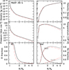	Fig. 5. Same as for Fig. 4, but for WASP-80 b.
In the text

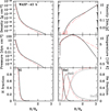	Fig. 6. Same as for Fig. 4, but for WASP-43 b.
In the text

Fig. 7. Simulated specific heating and cooling rate profiles for the atmosphere of HD 97658 b, broken into individual, contributing mechanism (see legend for details); the dark and light gray curves, respectively, trace the photo-heating and cooling rates obtained by TPCI (S16). In the case of the low-gravity, low-irradiation planet HD 97658 b, atmospheric escape is driven by adiabatic expansion, with negligible contribution from radiative cooling.

In the text

	Fig. 8. Same as for Fig. 7, but for WASP-80 b. In the case of this moderate-gravity, moderate-irradiation planet, atmospheric escape is mainly driven by radiative cooling in the innermost region, albeit with a non-negligible contribution from adiabatic expansion; further out, where the ionization fraction approaches 100%, adiabatic expansion takes over and dominates the cooling.
In the text

	Fig. 9. Same as for Fig. 7, but for WASP-43 b. In the case of this high-gravity, high-irradiation planet, atmospheric escape is entirely driven by radiative cooling in the innermost region; only further out, where the ionization fraction approaches 100%, adiabatic expansion takes over and dominates the cooling.
In the text

Fig. 10. Simulated, steady-state mass outflow rates from the 14 planetary systems considered in this work. The values obtained by ATES (in black) are compared to those by TPCI (S16, in red). Overall, the estimated mass loss rates agree to within a factor of 2 in all cases. In those cases where ATES differs from TPCI, the differences are always upward, and are likely due to inclusion of ion advection, which ATES implements in post-processing, yielding systematically higher atmospheric density profiles. This implementation choice, however, is chiefly responsible for the dramatic gain in computational time.

In the text

Fig. 11. All the planetary systems simulated in this study are shown in the (Φp, FXUV) plane, and color-coded based on the estimated mass loss rate illustrated by the right-hand side bar. Open, color-less circles show those cases for which ATES fails to converge. In general, known planets are identified by their names and highlighted by a circle; all the others are “synthetic”. ATES recovers stable, steady-state solutions for systems with log(−Φp)≲12.9 + 0.17 log FXUV (in cgs units); such convergence threshold is marked by the dashed black line.

In the text

References

- Allan, A., & Vidotto, A. A. 2019, MNRAS, 490, 3760 [Google Scholar]
- Batten, P., Clarke, N., Lambert, C., & Causon, D. M. 1997, SIAM J. Sci. Comput., 18, 1553 [CrossRef] [Google Scholar]
- Bisikalo, D. V., Shematovich, V. I., Cherenkov, A. A., Fossati, L., & Möstl, C. 2018, ApJ, 869, 108 [NASA ADS] [CrossRef] [Google Scholar]
- Bourrier, V., Lecavelier des Etangs, A., Dupuy, H., et al. 2013, A&A, 551, A63 [NASA ADS] [CrossRef] [EDP Sciences] [Google Scholar]
- Chadney, J. M., Galand, M., Unruh, Y. C., Koskinen, T. T., & Sanz-Forcada, J. 2015, Icarus, 250, 357 [Google Scholar]
- Chen, H., & Rogers, L. A. 2016, ApJ, 831, 180 [Google Scholar]
- Cubillos, P., Erkaev, N. V., Juvan, I., et al. 2017, MNRAS, 466, 1868 [Google Scholar]
- Debrecht, A., Carroll-Nellenback, J., Frank, A., et al. 2019, MNRAS, 483, 1481 [NASA ADS] [CrossRef] [Google Scholar]
- Debrecht, A., Carroll-Nellenback, J., Frank, A., et al. 2020, MNRAS, 493, 1292 [Google Scholar]
- Ehrenreich, D., & Désert, J. M. 2011, A&A, 529, A136 [NASA ADS] [CrossRef] [EDP Sciences] [Google Scholar]
- Ehrenreich, D., Bourrier, V., Wheatley, P. J., et al. 2015, Nature, 522, 459 [Google Scholar]
- Erkaev, N. V., Kulikov, Yu. N., Lammer, H., et al. 2007, A&A, 472, 329 [NASA ADS] [CrossRef] [EDP Sciences] [Google Scholar]
- Erkaev, N. V., Lammer, H., Odert, P., et al. 2013, Astrobiology, 13, 1011 [Google Scholar]
- Erkaev, N. V., Lammer, H., Odert, P., Kulikov, Y. N., & Kislyakova, K. G. 2015, MNRAS, 448, 1916 [NASA ADS] [CrossRef] [Google Scholar]
- Erkaev, N. V., Lammer, H., Odert, P., et al. 2016, MNRAS, 460, 1300 [NASA ADS] [CrossRef] [Google Scholar]
- Erkaev, N. V., Odert, P., Lammer, H., et al. 2017, MNRAS, 470, 4330 [NASA ADS] [CrossRef] [Google Scholar]
- Esquivel, A., Raga, A. C., Cantó, J., & Rodríguez-González, A. 2009, A&A, 507, 855 [NASA ADS] [CrossRef] [EDP Sciences] [Google Scholar]
- Esquivel, A., Schneiter, M., Villarreal D’Angelo, C., Sgró, M. A., & Krapp, L. 2019, MNRAS, 487, 5788 [NASA ADS] [CrossRef] [Google Scholar]
- Ferland, G. J., Korista, K. T., Verner, D. A., et al. 1998, PASP, 110, 761 [Google Scholar]
- Fossati, L., Erkaev, N. V., Lammer, H., et al. 2017, A&A, 598, A90 [NASA ADS] [CrossRef] [EDP Sciences] [Google Scholar]
- Fulton, B. J., Petigura, E. A., Howard, A. W., et al. 2017, AJ, 154, 109 [Google Scholar]
- García Muñoz, A. 2007, Planet. Space Sci., 55, 1426 [Google Scholar]
- Glover, S. C. O., & Jappsen, A.-K. 2007, ApJ, 666, 1 [NASA ADS] [CrossRef] [Google Scholar]
- Gottlieb, S., & Shu, C. W. 1998, Math. Comput., 67, 73 [NASA ADS] [CrossRef] [Google Scholar]
- Hui, L., & Gnedin, N. Y. 1997, MNRAS, 292, 27 [Google Scholar]
- Ionov, D. E., Shematovich, V. I., & Pavlyuchenkov, Y. N. 2017, Astron. Rep., 61, 387 [NASA ADS] [CrossRef] [Google Scholar]
- Jaritz, G. F., Endler, S., Langmayr, D., et al. 2005, A&A, 439, 771 [NASA ADS] [CrossRef] [EDP Sciences] [Google Scholar]
- Jin, S., & Mordasini, C. 2018, ApJ, 853, 163 [Google Scholar]
- Khodachenko, M. L., Shaikhislamov, I. F., Lammer, H., et al. 2017, ApJ, 847, 126 [CrossRef] [Google Scholar]
- Khodachenko, M. L., Shaikhislamov, I. F., Lammer, H., et al. 2019, ApJ, 885, 67 [NASA ADS] [CrossRef] [Google Scholar]
- Koskinen, T. T., Aylward, A. D., & Miller, S. 2007, Nature, 450, 845 [CrossRef] [Google Scholar]
- Koskinen, T. T., Harris, M. J., Yelle, R. V., & Lavvas, P. 2013, Icarus, 226, 1678 [Google Scholar]
- Koskinen, T. T., Lavvas, P., Harris, M. J., & Yelle, R. V. 2014, Phil. Trans. R. Soc. London Ser. A, 372, 20130089 [Google Scholar]
- Krenn, A. F., Fossati, L., Kubyshkina, D., & Lammer, H. 2021, A&A, 650, A94 [NASA ADS] [CrossRef] [EDP Sciences] [Google Scholar]
- Kubyshkina, D. I., & Fossati, L. 2021, Res. Notes Am. Astron. Soc., 5, 74 [Google Scholar]
- Kubyshkina, D., Fossati, L., Erkaev, N. V., et al. 2018a, ApJ, 866, L18 [NASA ADS] [CrossRef] [Google Scholar]
- Kubyshkina, D., Fossati, L., Erkaev, N. V., et al. 2018b, A&A, 619, A151 [NASA ADS] [CrossRef] [EDP Sciences] [Google Scholar]
- Kubyshkina, D., Vidotto, A. A., Fossati, L., & Farrell, E. 2020, MNRAS, 499, 77 [Google Scholar]
- Kulow, J. R., France, K., Linsky, J., & Loyd, R. O. P. 2014, ApJ, 786, 132 [Google Scholar]
- Kurganov, A., & Tadmor, E. 2000, J. Comput. Phys., 160, 241 [NASA ADS] [CrossRef] [Google Scholar]
- Lammer, H., Selsis, F., Ribas, I., et al. 2003, ApJ, 598, L121 [Google Scholar]
- Lammer, H., Odert, P., Leitzinger, M., et al. 2009, A&A, 506, 399 [NASA ADS] [CrossRef] [EDP Sciences] [Google Scholar]
- Lammer, H., Erkaev, N. V., Fossati, L., et al. 2016, MNRAS, 461, L62 [Google Scholar]
- Lecavelier des Etangs, A., Vidal-Madjar, A., McConnell, J. C., & Hébrard, G. 2004, A&A, 418, L1 [NASA ADS] [CrossRef] [EDP Sciences] [Google Scholar]
- Lecavelier des Etangs, A., Ehrenreich, D., Vidal-Madjar, A., et al. 2010, A&A, 514, A72 [NASA ADS] [CrossRef] [EDP Sciences] [Google Scholar]
- LeVeque, R. 2002, Finite Volume Methods for Hyperbolic Problems, Cambridge Texts in Applied Mathematics (Cambridge: Cambridge University Press) [CrossRef] [Google Scholar]
- Lopez, E. D., Fortney, J. J., & Miller, N. 2012, ApJ, 761, 59 [Google Scholar]
- Mayor, M., & Queloz, D. 1995, Nature, 378, 355 [Google Scholar]
- McCann, J., Murray-Clay, R. A., Kratter, K., & Krumholz, M. R. 2019, ApJ, 873, 89 [NASA ADS] [CrossRef] [Google Scholar]
- Mignone, A., Zanni, C., Tzeferacos, P., et al. 2012, ApJS, 198, 7 [Google Scholar]
- Murray-Clay, R. A., Chiang, E. I., & Murray, N. 2009, ApJ, 693, 23 [Google Scholar]
- Odert, P., Erkaev, N. V., Kislyakova, K. G., et al. 2020, A&A, 638, A49 [EDP Sciences] [Google Scholar]
- Owen, J. E. 2019, ARA&A, 47, 67 [Google Scholar]
- Owen, J. E., & Jackson, A. P. 2012, MNRAS, 425, 2931 [Google Scholar]
- Owen, J. E., & Morton, T. D. 2016, ApJ, 819, L10 [NASA ADS] [CrossRef] [Google Scholar]
- Owen, J. E., & Wu, Y. 2013, ApJ, 775, 105 [Google Scholar]
- Owen, J. E., & Wu, Y. 2016, ApJ, 817, 107 [NASA ADS] [CrossRef] [Google Scholar]
- Owen, J. E., & Wu, Y. 2017, ApJ, 847, 29 [Google Scholar]
- Paxton, B., Smolec, R., Schwab, J., et al. 2019, ApJS, 243, 10 [Google Scholar]
- Powell, M. J. D. 1970, in Numerical Methods for Nonlinear Algebraic Equations, ed. P. Rabinowitz (New York: Gordon and Breach), 87 [Google Scholar]
- Ribas, I., Guinan, E. F., Gudel, M., & Audard, M. 2005, ApJ, 622, 680 [NASA ADS] [CrossRef] [Google Scholar]
- Roe, P. 1981, J. Comput. Phys., 43, 357 [NASA ADS] [CrossRef] [Google Scholar]
- Rusanov, V. 1962, Calculation of Interaction of Non-steady Shock Waves with Obstacles, Technical Translation (National Research Council of Canada) [Google Scholar]
- Salz, M., Banerjee, R., Mignone, A., et al. 2015, A&A, 576, A21 [NASA ADS] [CrossRef] [EDP Sciences] [Google Scholar]
- Salz, M., Czesla, S., Schneider, P. C., & Schmitt, J. H. M. M. 2016, A&A, 586, A75 [NASA ADS] [CrossRef] [EDP Sciences] [Google Scholar]
- Sedov, L. I. 1959, Similarity and Dimensional Methods in Mechanics (New York: Academic Press) [Google Scholar]
- Sekiya, M., Nakazawa, K., & Hayashi, C. 1980, Prog. Theor. Phys., 64, 1968 [CrossRef] [Google Scholar]
- Shaikhislamov, I. F., Khodachenko, M. L., Sasunov, Y. L., et al. 2014, ApJ, 795, 132 [NASA ADS] [CrossRef] [Google Scholar]
- Shematovich, V. I. 2010, Sol. Syst. Res., 44, 96 [NASA ADS] [CrossRef] [Google Scholar]
- Showman, A. P., Lewis, N. K., & Fortney, J. J. 2015, ApJ, 801, 95 [NASA ADS] [CrossRef] [Google Scholar]
- Spake, J. J., Sing, D. K., Evans, T. M., et al. 2018, Nature, 557, 68 [Google Scholar]
- Stone, J. M., Gardiner, T. A., Teuben, P., Hawley, J. F., & Simon, J. B. 2008, ApJS, 178, 137 [NASA ADS] [CrossRef] [Google Scholar]
- Strömgren, B. 1939, ApJ, 89, 526 [CrossRef] [Google Scholar]
- Tian, F., Toon, O., Pavlov, A., & De Sterck, H. 2005, ApJ, 621, 1049 [NASA ADS] [CrossRef] [Google Scholar]
- Toro, E. 2009, Riemann Solvers and Numerical Methods for Fluid Dynamics: A Practical Introduction (Berlin, Heidelberg: Springer-Verlag) [CrossRef] [Google Scholar]
- Toro, E. F., Spruce, M., & Speares, W. 1994, Shock Waves, 4, 25 [Google Scholar]
- Vidal-Madjar, A., Lecavelier des Etangs, A., Désert, J. M., et al. 2003, Nature, 422, 143 [Google Scholar]
- Vidotto, A. A., & Cleary, A. 2020, MNRAS, 494, 2417 [Google Scholar]
- Watson, A., Donahue, T., & Walker, J. 1981, Icarus, 48, 150 [NASA ADS] [CrossRef] [Google Scholar]
- Yamaleev, N. K., & Carpenter, M. H. 2009, J. Comput. Phys., 228, 3025 [NASA ADS] [CrossRef] [Google Scholar]
- Yelle, R. V. 2004, Icarus, 170, 167 [NASA ADS] [CrossRef] [Google Scholar]