© ESO 2021

1. Introduction

The theory of the generation and transfer of polarized radiation is of crucial importance for solar and stellar physics. Currently, one of the main challenges in the field is performing detailed numerical simulations of the transfer of polarized radiation in magnetized and dynamic atmospheres. In particular, it is essential to properly account for scattering processes in complex atomic models and multidimensional geometries, which lead to nonlinear and nonlocal multidimensional problems. In applied science, it is often profitable to convert nonlinear problems into linear ones, allowing the use of the powerful tools from numerical linear algebra, such as stationary or Krylov iterative methods. This is also the case in the field of numerical radiative transfer, where a fair number of problems of practical interest are accurately described through a linear system. For instance, the modeling of the transfer of resonance line polarization considering two-level (or two-term) atomic models can be linearized by assuming that the lower level (or term) is not polarized and that its population is known and fixed a priori (see, e.g., Belluzzi & Trujillo Bueno 2014; Sampoorna et al. 2017; Alsina Ballester et al. 2017).

In principle, linear problems can be solved in a single step with a direct method. However, this task can be highly inefficient or even unfeasible in practice, especially for large problems. Therefore, it is common to rely on efficient stationary iterative methods that, combined with suitable parallelization strategies, make the whole problem computationally tractable.

Trujillo Bueno & Landi Degl’Innocenti (1996) first applied the Richardson (a.k.a. fixed point iteration), Jacobi, and block-Jacobi iterative methods to the numerical transfer of polarized radiation¹, while Trujillo Bueno & Manso Sainz (1999) applied Gauss-Seidel and successive over-relaxation (SOR) iterative methods to the same problem. In particular, the block-Jacobi iterative method is still frequently used in different scattering polarization problems (e.g., Belluzzi & Trujillo Bueno 2014; Alsina Ballester et al. 2017; Sampoorna et al. 2017; Alsina Ballester et al. 2018). By contrast, Gauss-Seidel and SOR iterative methods are not of common practice (Lambert et al. 2016), because they are nontrivial to parallelize. Despite of its slow convergence, the Richardson iterative method is still used in computationally complex transfer problems, where the other iterative methods are not exploitable (e.g., del Pino Alemán et al. 2020; Janett et al. 2021).

A rigorous investigation of the convergence conditions of such iterative methods applied to transfer problems of polarized radiation is still lacking. The specific stability requirements are problem-dependent and often difficult to determine. This paper gives a deeper analysis of these convergence conditions, analyzing their dependence on different design elements, such as the formal solver, the spectral, angular, and spatial numerical grids, and the damping factor.

Section 2 briefly introduces iterative methods, exposes their convergence conditions, and presents the most common stationary methods. Section 3 presents the benchmark analytical problem employed in this paper and exposes its discretization and algebraic formulation in the context of various iterative methods. Section 4 numerically analyzes the impact of different problem elements on the iterative solutions, focusing on the choice of the formal solver, on the various discrete grids, and on damping parameters. Finally, Sect. 5 provides remarks and conclusions, which are also generalized to more complex problems.

2. Iterative methods

We consider the linear system

$$\begin{array}{c}\hfill A\mathbf{x}=\mathbf{b},\end{array}$$(1)

where the nonsingular matrix $A\in {\mathbb{R}}^{N\times N}$ and the vector $\mathbf{b}\in {\mathbb{R}}^N$ are given, and the solution $\mathbf{x}\in {\mathbb{R}}^N$ is to be found. In absence of rounding errors, direct methods give the exact solution to the linear system (1) by a finite sequence of steps. They provide the solution

$$\begin{array}{c}\hfill \mathbf{x}=A^{-1}\mathbf{b},\end{array}$$

using, for example, a suitable factorization of A, using Gaussian elimination. Due to their high computational complexity and storage costs, direct methods are often prohibitive in practice, especially for large problems. For this reason, iterative methods are usually preferred for the solution of large linear systems. These methods are convenient in terms of parallel implementation and therefore particularly suitable for today’s high performance computing systems.

Iterative methods start with an initial guess ${\mathbf{x}}^0\in {\mathbb{R}}^N$ and generate a sequence of improving approximate solutions ${\mathbf{x}}^1,{\mathbf{x}}^2,\cdots ,{\mathbf{x}}^n,{\mathbf{x}}^{n+1}\in {\mathbb{R}}^N$ given by

$$\begin{array}{cc}& {\mathbf{x}}^1={\varphi }_0({\mathbf{x}}^0;A,\mathbf{b}),\hfill \\ \hfill & {\mathbf{x}}^2={\varphi }_1({\mathbf{x}}^0,{\mathbf{x}}^1;A,\mathbf{b}),\hfill \\ \hfill & ⋮\hfill \\ \hfill & {\mathbf{x}}^{n+1}={\varphi }_n({\mathbf{x}}^0,{\mathbf{x}}^1,\cdots ,{\mathbf{x}}^n;A,\mathbf{b}).\hfill \end{array}$$

A one-step iterative method computes the approximate solution xⁿ⁺¹ by considering only the previous approximate solution xⁿ. Hence, the transition from xⁿ to xⁿ⁺¹ does not rely on the previous history of the iterative process. Moreover, a stationary iterative method generates the sequence of approximate solutions by the recursive application of the same operator ϕ. Therefore, stationary one-step iterative methods can be expressed in the form

$$\begin{array}{c}\hfill {\mathbf{x}}^{n+1}=\varphi ({\mathbf{x}}^n;A,\mathbf{b}).\end{array}$$

If the operator ϕ is also linear, the linear stationary one-step iterative method can be expressed in the form

$$\begin{array}{c}\hfill {\mathbf{x}}^{n+1}=G{\mathbf{x}}^n+\mathbf{g},\end{array}$$(2)

where neither the iteration matrix $G\in {\mathbb{R}}^{N\times N}$ nor the vector g depend upon the iteration n. Hence, a linear stationary one-step iterative method starts from an initial guess x⁰ and repeatedly invokes the recursive formula (2) until a chosen termination condition matches (cf. Sect. 2.4).

In order to study and design linear stationary one-step iterative methods, it is convenient to consider the linear system (1) in the form

$$\begin{array}{c}\hfill \mathbf{x}=G\mathbf{x}+\mathbf{g}.\end{array}$$(3)

We recall that multistep iterative methods have been also used in the radiative transfer context. Relaying on multiple previous iterates, multistep iterative methods can accelerate the convergence of one-step iterations. In this regard, we mention Ng (e.g., Olson et al. 1986), ORTHOMIN (e.g., Klein et al. 1989), and state-of-the-art Krylov methods. In particular, Krylov acceleration strategies are the subject of the second part of this paper series (Benedusi et al. 2021).

2.1. Convergence conditions

An iterative method is convergent if the approximate solution xⁿ converges to the exact solution x as the iteration process progresses, that is, if xⁿ → x for n → ∞. This implies that the error, defined as

$$\begin{array}{c}\hfill {\mathbf{e}}^n={\mathbf{x}}^n-\mathbf{x},\end{array}$$

must approach zero as n increases. Subtracting Eq. (3) from Eq. (2), one obtains

$$\begin{array}{c}\hfill {\mathbf{e}}^{n+1}=G{\mathbf{e}}^n,\end{array}$$

indicating that the convergence of the iterative method depends entirely on the iteration matrix G. In fact, the iterative method (2) is convergent for any initial guess x⁰ if and only if

$$\begin{array}{c}\hfill \rho (G)<1,\end{array}$$(4)

where ρ(G) is the spectral radius of G (see, e.g., Hackbusch 2016). The quantity ρ(G) is also known as the convergence rate, because it describes the speed of convergence of an iterative process. When employing an iterative method, a rigorous convergence analysis based on the condition (4) is advisable. However, since an analytical expression of ρ(G) is often hard to obtain in practice, heuristic-based analyses are commonly employed to study how the convergence of iterative methods depends on problem and discretization parameters (Hackbusch 2016).

2.2. Examples

Linear stationary one-step iterative methods for the solution of (1) usually arise from the splitting

$$\begin{array}{c}\hfill A=P-R,\end{array}$$(5)

with P nonsingular. Rewriting Eq. (1) in the form of Eq. (3) and introducing iteration indices as in Eq. (2), one obtains

$$\begin{array}{c}\hfill {\mathbf{x}}^{n+1}=P^{-1}R{\mathbf{x}}^n+P^{-1}\mathbf{b},\end{array}$$(6)

with G = P⁻¹R = P⁻¹(P−A) = Id − P⁻¹A and g = P⁻¹b. Crucially, P has to be easier to invert then A, while being a good approximation of it to ensure fast convergence.

Sometimes, it is convenient to express iterative methods in terms of the correction

$$\begin{array}{c}\hfill \mathit{\delta }{\mathbf{x}}^n={\mathbf{x}}^{n+1}-{\mathbf{x}}^n.\end{array}$$

In the correction form, the iterative method (6) reads

$$\begin{array}{c}\hfill {\mathbf{x}}^{n+1}=(Id-P^{-1}A){\mathbf{x}}^n+P^{-1}\mathbf{b}={\mathbf{x}}^n+P^{-1}(\mathbf{b}-A{\mathbf{x}}^n),\end{array}$$

or simply

$$\begin{array}{c}\hfill {\mathbf{x}}^{n+1}={\mathbf{x}}^n+\mathit{\delta }{\mathbf{x}}^n,\end{array}$$(7)

where the correction is given by δxⁿ = P⁻¹rⁿ and rⁿ = b − Axⁿ is the iteration residual.

Many iterative methods are defined through the following decomposition of the matrix A

$$\begin{array}{c}\hfill A=D+L+U,\end{array}$$

where D is the diagonal of A, while L and U are its strict lower and strict upper triangular parts, respectively. Different choices of the matrix P yield different iterative methods:

$$\begin{array}{ccc}\hfill P& =Id,\hfill & \text{Richardson method},\hfill \\ \hfill P& =D,\hfill & \text{Jacobi method},\hfill \\ \hfill P& =\text{blockdiag}(A_1,\dots ,A_m),\hfill & \text{block-Jacobi method},\hfill \\ \hfill P& =D+L\text{or}P=D+U,\hfill & \text{Gauss-Seidel method},\hfill \end{array}$$

with A₁, …, A_m being m square diagonal blocks of A. All these choices of P allow for a convenient, and possibly parallel, computation of P⁻¹. We note that the iterative method corresponding to P = A always converges in one iteration, resulting in a direct method.

In another perspective, known as preconditioning, all these methods correspond to a Richardson iteration applied to the preconditioned system

$$\begin{array}{c}\hfill P^{-1}A\mathbf{x}=P^{-1}\mathbf{b},\end{array}$$(8)

which is equivalent to the linear system (1). The nonsingular matrix P is known as preconditioner and is usually chosen to reduce the condition number of P⁻¹A with respect to the one of A, such that the preconditioned system is “easier” to solve with respect to the original one.

Multiplying the preconditioner P (or part of it) by a positive scalar, leads to damped iterative schemes, which are discussed in the following section.

2.3. Damped iterative methods

The classical idea of damping (or relaxation) consists in scaling the correction δxⁿ in Eq. (7) by a damping factor $\omega \in {\mathbb{R}}_{>0}$, namely

$$\begin{array}{c}\hfill {\mathbf{x}}^{n+1}={\mathbf{x}}^n+\omega \mathit{\delta }{\mathbf{x}}^n={\mathbf{x}}^n+\omega P^{-1}{\mathbf{r}}^n.\end{array}$$(9)

The term damped properly holds only for 0 < ω < 1, a.k.a. under-relaxation. In fact, the choice ω = 1 yields the original method, while ω > 1 gives an extrapolated version, a.k.a. over-relaxation. For simplicity, the term damped will be used for all choices of ω. Damped iterations can also be read as

$$\begin{array}{c}\hfill {\mathbf{x}}^{n+1}={\mathbf{x}}^n-\omega {\mathbf{x}}^n+\omega {\mathbf{x}}^n+\omega \mathit{\delta }{\mathbf{x}}^{n+1}=(1-\omega ){\mathbf{x}}^n+\omega {\stackrel{\sim }{\mathbf{x}}}^{n+1},\end{array}$$

that is, the weighted mean of the old iterate xⁿ and one step of the original method ${\stackrel{\sim }{\mathbf{x}}}^{n+1}={\mathbf{x}}^n+\mathit{\delta }{\mathbf{x}}^n$.

In order to guarantee the convergence of damped methods, it is possible to obtain bounds on ω as well as optimal choices in terms of convergence rate. In particular, the preconditioned iteration (9) is convergent if and only if

$$\begin{array}{c}\hfill \omega <\frac{2\text{Re}({\lambda }_i)}{|{\lambda }_i{|}^2},\mathrm{for}\mathrm{all}i=1,\dots ,N,\end{array}$$(10)

λ_i being the ith eigenvalue of the matrix P⁻¹A. If P⁻¹A has real positive eigenvalues, the optimal convergence rate for the iterative methods presented in Sect. 2.2 is attained for

$$\begin{array}{c}\hfill {\omega }_{\text{opt}}=\frac{2}{{\lambda }_{min}+{\lambda }_{max}},\end{array}$$(11)

where λ_min and λ_max are the minimum and maximum eigenvalues of P⁻¹A. The SOR method is a damped variant of the Gauss-Seidel method, with P = ω⁻¹D + L. If A is consistently ordered, G_Jac = Id − D⁻¹A has real eigenvalues, and ρ(G_Jac) < 1, the optimal convergence rate for SOR is attained for

$$\begin{array}{c}\hfill {\omega }_{\text{sor}}=1+{\left(\frac{\rho (G_{\text{Jac}})}{1+\sqrt{1-\rho {(G_{\text{Jac}})}^2}}\right)}^2.\end{array}$$(12)

A deeper and comprehensive analysis of damped stationary iterative methods is given, for instance, by Hageman & Young (1981), Saad (2003), Quarteroni et al. (2010), Hackbusch (2016).

2.4. Termination condition

Typically, iterative solution strategies terminate at the nth step if the norm of the relative residual is smaller then a desired tolerance, that is, if ‖rⁿ‖₂/‖b‖₂ < tol. However, this stopping criteria becomes less and less reliable as the condition number of A, denoted with κ(A), increases. In fact, the following relation between the relative error and the relative residual holds:

$$\begin{array}{c}\hfill \Vert \mathbf{x}-{\mathbf{x}}^n{\Vert }_2/{\Vert \mathbf{x}\Vert }_2\le \kappa (A)\Vert {\mathbf{r}}^n{\Vert }_2/{\Vert \mathbf{b}\Vert }_2.\end{array}$$

Since by construction κ(P⁻¹A) < κ(A), the same termination condition with respect to the preconditioned system (8), namely, ‖P⁻¹rⁿ‖₂/‖P⁻¹b‖₂ < tol, gives a better approximation of the true relative error.

3. Benchmark problem

In this section, we present the continuous formulation of a linear benchmark transfer problem for polarized radiation. Secondly, we consider its discretization and derive its algebraic formulation. Finally, we remark how the stationary iterative methods presented in Sects. 2.2 and 2.3 are applied in this context.

The problem is formulated within the framework of the theoretical approach described in Landi Degl’Innocenti & Landolfi (2004). Within this theory, a scattering process is treated as a succession of independent absorption and reemission processes. This is the so-called limit of complete frequency redistribution (CRD), in which no frequency correlations between the incoming and the outgoing photons in a scattering process are taken into account. We consider a two-level atom with an unpolarized lower level. Since stimulated emission is completely negligible in solar applications, it is not considered. For the sake of simplicity, the contribution of continuum processes is neglected, as well as that of magnetic and bulk velocity fields. We note, however, that the methodology presented in this section can also be applied to a wider range of settings, such as the unpolarized case, two-term atomic models including continuum contributions, atmospheric models with arbitrary magnetic and bulk velocity fields, and theoretical frameworks accounting for partial frequency redistribution (PRD) effects.

3.1. Continuous problem

The physical quantities entering the radiative transfer problem are, in general, functions of the spatial point r, the frequency ν, and the propagation direction Ω of the radiation ray under consideration. In the absence of polarization phenomena, the specific intensity and the atomic level population fully describe the radiation field and the atomic system, respectively. When polarization is taken into account, a more detailed description is instead required. The radiation field is fully described by the four Stokes parameters

$$\begin{array}{c}\hfill I_i(\mathit{r},\mathrm{\Omega },\nu ),\end{array}$$

with i = 1, …, 4, standing for Stokes I, Q, U, and V, respectively. The nth energy level of the atomic system, with total angular momentum J_n, is fully described by the multipolar components of the density matrix, a.k.a. spherical statistical tensors,

$$\begin{array}{c}\hfill {\rho }_{Q,n}^K(\mathit{r}),\end{array}$$

with K = 0, …, 2J_n, and Q = −K, …, K. We recall that the spherical statistical tensors are in general complex quantities, and that the 0-rank component, ${\rho }_{0,n}^0$, is proportional to the population of the nth level (see Landi Degl’Innocenti & Landolfi 2004, Chapt. 3). A two-level atomic system at position r is thus described by the following quantities

$$\begin{array}{c}\hfill {\rho }_{Q,\ell }^K(\mathit{r}),\mathrm{and}{\rho }_{Q,u}^K(\mathit{r}),\end{array}$$

with the subscripts ℓ and u indicating the lower and upper levels, respectively. The assumption of unpolarized lower level² implies that

$$\begin{array}{c}\hfill {\rho }_{Q,\ell }^K(\mathit{r})={\rho }_{0,\ell }^0(\mathit{r}){\delta }_{K0}{\delta }_{Q0},\end{array}$$

where δ_ij is the Kronecker delta.

In the absence of magnetic fields, the statistical equilibrium equations of a two-level atom with an unpolarized lower level have the following analytical solution (see Landi Degl’Innocenti & Landolfi 2004, Chapt. 14)³:

$$\begin{array}{cc}& \frac{{\rho }_{Q,u}^K(\mathit{r})}{{\rho }_{0,\ell }^0(\mathit{r})}=\sqrt{\frac{2J_u+1}{2J_{\ell }+1}}\frac{c^2}{2h{\nu }_0^3}[a_{J_u{J}_{\ell }}^{(K,Q)}(\mathit{r}){\overline{J}}_{-Q}^K(\mathit{r})+ϵ(\mathit{r})W(\mathit{r}){\delta }_{K0}{\delta }_{Q0}],\hfill \end{array}$$(13)

where c and h have their usual meaning of light speed and Planck constant, respectively, ϵ is the so-called thermalization parameter, W is the Planck function in the Wien limit at the line-center frequency ν₀, and

$$\begin{array}{c}\hfill a_{J_u{J}_{\ell }}^{(K,Q)}(\mathit{r})={(-1)}^Q\frac{(1-ϵ(\mathit{r}))w_{J_u{J}_{\ell }}^{(K)}}{1+{\delta }_u^{(K)}(\mathit{r})(1-ϵ(\mathit{r}))}.\end{array}$$

The coefficient $w_{J_u{J}_{\mathcal{l}}}^{(K)}$ is the polarizability factor⁴, ${\delta }_u^{(K)}$ describes the depolarizing rate of the upper level due to elastic collisions, and the frequency-averaged radiation field tensor is given by

$$\begin{array}{c}\hfill {\overline{J}}_Q^K(\mathit{r})={\displaystyle \int }\mathrm{d}\nu \varphi (\mathit{r},\nu )\frac{1}{4\pi }{\displaystyle \oint }\mathrm{d}\mathrm{\Omega }{\displaystyle \sum _{i=1}^4{\mathcal{T}}_{Q,i}^K(\mathrm{\Omega })I_i(\mathit{r},\mathrm{\Omega },\nu ),}\end{array}$$(14)

where ${\mathcal{T}}_{Q,i}^K(\mathbf{\Omega })$ is the polarization tensor (see Landi Degl’Innocenti & Landolfi 2004, Chapt. 5) and ϕ is the absorption profile. By definition, the maximum rank of the radiation field tensor ${\overline{J}}_Q^K$ is K = 2 (see Landi Degl’Innocenti & Landolfi 2004, Chapt. 5). Consequently, the only nonzero spherical statistical tensors of the upper level ${\rho }_{Q,u}^K$ are those with K ≤ 2. Exploiting the conjugation properties of the spherical statistical tensors (see Landi Degl’Innocenti & Landolfi 2004, Chapt. 3), at each position r, the considered two-level atomic system with an unpolarized lower level is thus described by 9 real quantities.

The propagation of the Stokes parameters at frequency ν along Ω is described by the following differential equation

$$\begin{array}{c}\hfill \frac{\mathrm{d}}{\mathrm{d}s}{I}_i(\mathit{r},\mathbf{\Omega },\nu )=-{\displaystyle \sum _{j=1}^4{K}_{\mathit{ij}}(\mathit{r},\mathbf{\Omega },\nu )I_j(\mathit{r},\mathbf{\Omega },\nu )+{\epsilon }_i(\mathit{r},\mathbf{\Omega },\nu ),}\end{array}$$

where s is the spatial coordinate along the direction Ω, ε_i is the emission coefficient of the ith Stokes parameter, and the entries K_ij form the 4 × 4 propagation matrix.

In the absence of a magnetic field and lower level polarization, the propagation matrix is diagonal with diagonal element η. The transfer equations for the four Stokes parameters are consequently decoupled and read

$$\begin{array}{c}\hfill \frac{\mathrm{d}}{\mathrm{d}s}{I}_i(\mathit{r},\mathbf{\Omega },\nu )=-\eta (\mathit{r},\nu )[I_i(\mathit{r},\mathbf{\Omega },\nu )-S_i(\mathit{r},\mathbf{\Omega })].\end{array}$$(15)

We note that η does not depend on Ω because bulk velocity fields are neglected, while the source function S_​i does not depend on ν because of the CRD assumption. Considering dipole scattering and neglecting the continuum contribution, the source function for the ith Stokes parameter is given by (see Landi Degl’Innocenti & Landolfi 2004, Chapt. 14)

$$\begin{array}{c}\hfill S_i(\mathit{r},\mathbf{\Omega })=\frac{{\epsilon }_i(\mathit{r},\mathbf{\Omega },\nu )}{\eta (\mathit{r},\nu )}={\displaystyle \sum _{\mathit{KQ}}{w}_{J_u{J}_{\ell }}^{(K)}{\mathcal{T}}_{Q,i}^K(\mathbf{\Omega }){\sigma }_Q^K(\mathit{r}),}\end{array}$$(16)

with

$$\begin{array}{c}\hfill {\sigma }_Q^K(\mathit{r})=\frac{2h{\nu }_0^3}{c^2}\sqrt{\frac{2J_{\ell }+1}{2J_u+1}}\frac{{\rho }_{Q,u}^K(\mathit{r})}{{\rho }_{0,\ell }^0(\mathit{r})}.\end{array}$$(17)

Using Eq. (13), the quantities ${\sigma }_Q^K$, which can be interpreted as the multipolar components of the source function, are given by

$$\begin{array}{c}\hfill {\sigma }_Q^K(\mathit{r})=a_{J_u{J}_{\ell }}^{(K,Q)}(\mathit{r}){\overline{J}}_{-Q}^K(\mathit{r})+ϵ(\mathit{r})W(\mathit{r}){\delta }_{K0}{\delta }_{Q0}.\end{array}$$(18)

3.2. Discretization and algebraic formulation

In order to replace the continuous problem by a system of algebraic equations, we discretize the continuous variables ν, r, and Ω using, respectively, grids with N_ν, N_s and N_Ω nodes. The quantities of the problem are now evaluated at the nodes at ${\{{\mathbf{r}}_k\}}_{k=1}^{N_s}$, ${\left\{{\mathbf{\Omega }}_m\right\}}_{m=1}^{N_{\mathrm{\Omega }}}$, and ${\left\{{\nu }_p\right\}}_{p=1}^{N_{\nu }}$ only.

For k = 1, …, N_s, the quantity ${\sigma }_Q^K({\mathbf{r}}_k)$ is computed through the discrete versions of Eqs. (18) and (14), namely,

$$\begin{array}{c}\hfill {\sigma }_Q^K({\mathbf{r}}_k)={\displaystyle \sum _{i=1}^4\sum _{m=1}^{N_{\mathrm{\Omega }}}\sum _{p=1}^{N_{\nu }}{J}_{KQ,i}({\mathbf{r}}_k,{\mathrm{\Omega }}_m,{\nu }_p)I_i({\mathbf{r}}_k,{\mathrm{\Omega }}_m,{\nu }_p)+c_Q^K({\mathbf{r}}_k),}\end{array}$$(19)

where J_KQ,i(r_k,Ω_m,ν_p) depends on the choice of spectral and angular quadratures used in Eq. (14) (cf. Eq. (A.3)), while $c_Q^K({\mathbf{r}}_k)=ϵ({\mathbf{r}}_k)W({\mathbf{r}}_k){\delta }_{K0}{\delta }_{Q0}$.

Similarly, the discrete version of Eq. (16) reads

$$\begin{array}{c}\hfill S_i({\mathbf{r}}_k,{\mathrm{\Omega }}_m)={\displaystyle \sum _{\mathit{KQ}}{T}_{i,KQ}({\mathrm{\Omega }}_m){\sigma }_Q^K({\mathbf{r}}_k),}\end{array}$$(20)

with $T_{i,KQ}({\mathbf{\Omega }}_m)=w_{J_u{J}_{\mathcal{l}}}^{(K)}{\mathcal{T}}_{Q,i}^K({\mathbf{\Omega }}_m)$. Finally, provided initial conditions, the transfer equation (15) can be solved along each propagation direction Ω_m and at each frequency ν_p to provide the Stokes component I_i(r_k,Ω_m,ν_p) for all k. This numerical step can be expressed as

$$\begin{array}{cc}& I_i({\mathbf{r}}_k,{\mathrm{\Omega }}_m,{\nu }_p)={\displaystyle \sum _{l=1}^{N_s}{\mathrm{\Lambda }}_i({\mathbf{r}}_k,{\mathbf{r}}_l,{\mathrm{\Omega }}_m,{\nu }_p)S_i({{\mathbf{r}}_l,\mathrm{\Omega }}_m)}\hfill \\ \hfill & +t_i({\mathbf{r}}_k,{\mathrm{\Omega }}_m,{\nu }_p),\hfill \end{array}$$(21)

where t_i(r_k,Ω_m,ν_p) represents the radiation transmitted from the boundaries and the coefficients Λ_i(r_k,r_l,Ω_m,ν_p) encode the numerical method used to propagate the ith Stokes parameter along the ray Ω_m (cf. Eq. (C.9)). For notational simplicity, the explicit dependence on variables and indexes is omitted, and Eqs. (19)–(21) are expressed, respectively, in the following compact matrix form

$$\begin{array}{cc}& \mathit{\sigma }=J\mathbf{I}+\mathbf{c},\mathrm{with}J\in {\mathbb{R}}^{9N_s\times 4N_s{N}_{\mathrm{\Omega }}{N}_{\nu }},\hfill \end{array}$$(22)

$$\begin{array}{cc}& \mathbf{S}=T\mathit{\sigma },\mathrm{with}T\in {\mathbb{R}}^{4N_s{N}_{\mathrm{\Omega }}\times 9N_s},\hfill \end{array}$$(23)

$$\begin{array}{cc}& \mathbf{I}=\mathrm{\Lambda }\mathbf{S}+\mathbf{t},\mathrm{with}\mathrm{\Lambda }\in {\mathbb{R}}^{4N_s{N}_{\mathrm{\Omega }}{N}_{\nu }\times 4N_s{N}_{\mathrm{\Omega }}},\hfill \end{array}$$(24)

where the vector $\mathbf{I}\in {\mathbb{R}}^{4N_s{N}_{\mathrm{\Omega }}{N}_{\nu }}$ collects the discretized Stokes parameters, $\mathbf{S}\in {\mathbb{R}}^{4N_s{N}_{\mathrm{\Omega }}}$ the discretized source function, and $\mathit{\sigma }\in {\mathbb{R}}^{9N_s}$ its discretized multipolar components. The explicit expressions of vectors and matrices appearing in Eqs. (22)–(24) are given in Appendices A–C for a one-dimensional (1D) spatial grid. In general, the entries of the matrix J depend on the type of numerical integration used in Eq. (14), while the entries of T depend on the coefficients of Eq. (16). Moreover, the entries of Λ depend on the numerical method used to solve the transfer equation (15) (a.k.a. formal solver), on the spatial grid and, eventually, on the numerical conversion to the optical depth scale (e.g., Janett & Paganini 2018).

By choosing σ as the unknown vector, Eqs. (22)–(24) can then be combined into a single discrete problem, namely,

$$\begin{array}{c}\hfill (Id-J\mathrm{\Lambda }T)\mathit{\sigma }=J\mathbf{t}+\mathbf{c},\end{array}$$(25)

with Id − JΛT being a square matrix of size 9N_s.

The operator Λ and the vector t depend on the absorption coefficient η, which linearly depends on ${\rho }_{0,\mathcal{l}}^0$, which in turn enters the definition of the unknown σ. The discrete problem (25) is consequently nonlinear. However, the nonlinear problem (25) becomes linear if we further assume either that (i) the transfer equation (15) is solved by introducing the optical depth scale defined by

$$\begin{array}{c}\hfill \mathrm{d}\tau (\nu )=-\eta (\mathit{r},\nu )\mathrm{d}s,\end{array}$$

and the optical depth grid is fixed a priori, or that (ii) the density matrix element ${\rho }_{0,\mathcal{l}}^0$ (or equivalently the lower level atomic population) is fixed a priori and, consequently, the absorption coefficient η becomes a constant of the problem. We note that in both cases the operator Λ and the vector t become independent of the unknown σ.

In the literature, the so-called Λ-operator usually describes the mapping of the discretized source function vector S either to the specific intensity vector I or to the corresponding mean radiation field vector (e.g., Olson et al. 1986; Rybicki & Hummer 1991; Paletou & Auer 1995). This operator was introduced to highlight the linear nature of this mapping inside the whole nonlinear radiative transfer problem. The traditional Λ-operator corresponds either to Eq. (24) or to the combined action of Eq. (24) and the integral (14).

We note that the linearized system (25) has the same form as Eq. (1) with A = Id − JΛT, x = σ, and b = Jt + c. The matrix A can be assembled by constructing J, Λ, and T, computing the products JΛT, and finally calculating Id − JΛT. Alternatively, the matrix JΛT can be assembled column-by-column, constructing the jth column by applying Eqs. (19)–(21) (setting $c_q^K$ and t_i to zero) to a point-like multipolar component of the source function σ_i = δ_ij, for i, j = 1, …, 9N_s.

Applying the iterative methods exposed in Sect. 2.2 to Eq. (25), the following iteration matrix is obtained

$$\begin{array}{c}\hfill G=Id-P^{-1}(Id-J\mathrm{\Lambda }T),\end{array}$$(26)

P being an arbitrary preconditioner. Accordingly, the nth iteration in the correction form reads

$$\begin{array}{c}\hfill {\mathit{\sigma }}^{n+1}={\mathit{\sigma }}^n+\mathit{\delta }{\mathit{\sigma }}^n,\end{array}$$

where

$$\begin{array}{c}\hfill \mathit{\delta }{\mathit{\sigma }}^n=P^{-1}(J\mathrm{\Lambda }T{\mathit{\sigma }}^n-{\mathit{\sigma }}^n+J\mathbf{t}+\mathbf{c}).\end{array}$$

Sections 3.3–3.6 describe stationary iterative methods in the context of radiative transfer problems.

3.3. Richardson method

The form of the linear system (25) suggests the operator splitting Eq. (5) with P = Id and R = JΛT. The iterative method based on this splitting, that is,

$$\begin{array}{c}\hfill {\mathit{\sigma }}^{n+1}=J\mathrm{\Lambda }T{\mathit{\sigma }}^n+J\mathbf{t}+\mathbf{c},\end{array}$$(27)

is an example of the Richardson method, which is commonly known as Λ-iteration in the context of linear radiative transfer problems. Equation (27) describes the following iterative process: (i) given an initial estimate of σ, calculate S at each discrete position and direction through Eq. (16); (ii) compute the numerical solution of the transfer equation (15) to obtain I at each discrete position, frequency, and direction; (iii) integrate I at each position according to Eq. (14) to obtain the frequency averaged radiation field tensor, which is used to update σ using Eq. (18).

The damped Richardson method is simply obtained by multiplying the correction δσⁿ of the Richardson method by a damping factor ω.

3.4. Jacobi method

Considering Eq. (25), an usual operator splitting Eq. (5) is given by choosing the preconditioner P to be diagonal, with the same diagonal of Id − JΛT, resulting in a minimal cost for the application and computation of P⁻¹, possibly in parallel. This splitting yields the Jacobi method, while its damped version is obtained by multiplying the correction δσⁿ by a damping factor ω.

Trujillo Bueno & Manso Sainz (1999) applied the Jacobi method when dealing with CRD scattering line polarization linear problems. In this context, the Jacobi method is sometimes termed as ALI method or local ALI method (see Hubeny 2003). However, an increasing problem size results in a lower impact of the Jacobi acceleration. For instance, when PRD effects are included, the size of the resulting linear system scales with N_sN_ν under the angle-averaged approximation (see, e.g., Alsina Ballester et al. 2017), while it scales with N_sN_νN_Ω in the general angle-dependent treatment (see, e.g., Janett et al. 2021). In both cases, the impact of the Jacobi acceleration is barely perceptible.

3.5. Block-Jacobi method

In radiative transfer problems, linear systems often have a natural block structure, which offers different possibilities in defining the blocks. Appendices A–C explicitly illustrate the structure of the matrices that build up the linear system (25) for the 1D case. Considering Eq. (25), the preconditioner P can be chosen as the block-diagonal of Id − JΛT. This choice yields the block-Jacobi method, while its damped version is simply obtained by multiplying the correction δσⁿ by a damping factor ω. We remark that, within this method, the computation of P⁻¹ requires solving the multiple smaller systems corresponding to the diagonal blocks.

Trujillo Bueno & Manso Sainz (1999) first applied the block-Jacobi method to the CRD radiative transfer problem, choosing square blocks that account for the coupling of the different multipolar components of the source function. Moreover, the block-Jacobi method is a common choice when dealing with PRD radiative transfer problems under the angle-averaged approximation (e.g., Belluzzi & Trujillo Bueno 2014; Alsina Ballester et al. 2017; Sampoorna et al. 2017; Alsina Ballester et al. 2018). In this case, the preconditioner is usually built by square blocks of size N_ν that account for the coupling of all the frequencies (see the frequency-by-frequency method of Paletou & Auer 1995). In such applications, the block-Jacobi method is referred to as ALI, Jacobi, or Jacobi-based method. Janett et al. (2021) first applied the damped block-Jacobi method to the same problem.

3.6. Gauss-Seidel method

Another choice of the operator splitting Eq. (5) is given by choosing the preconditioner P as the lower (or upper) triangular part of Id − JΛT. This splitting yields the Gauss-Seidel method. The SOR method is simply obtained by modifying the correction δσⁿ with a suitable damping factor ω as explained in Sect. 2.3. Trujillo Bueno & Manso Sainz (1999) first proposed and applied the Gauss-Seidel and SOR methods to CRD scattering line polarization linear problems, while Sampoorna & Trujillo Bueno (2010) generalized these methods to the PRD case. Trujillo Bueno & Fabiani Bendicho (1995) confirmed with demonstrative results that the optimal parameter ω_sor given by Eq. (12) is indeed effective in the context of numerical radiative transfer. However, Gauss-Seidel and SOR methods are not common in radiative transfer applications (Lambert et al. 2016), mainly because they have limited and nontrivial parallelization capabilities (see, e.g., the red-black Gauss-Seidel algorithm Saad 2003).

4. Numerical analysis

It is worth mentioning that realistic radiative transfer problems can be substantially more complex than the one considered here. However, we present a suitable benchmark to better understand how the convergence of various iterative methods depends on different design elements, such as the choice of the formal solver, the discretization of the problem, or the use of damping factors. The conclusions could be then generalized to more complex problems.

In the absence of magnetic and bulk velocity fields, 1D plane-parallel atmospheres satisfy cylindrical symmetry with respect to the vertical. Due to the symmetry of the problem, the only nonzero radiation field tensor components are ${\overline{J}}_0^0$ and ${\overline{J}}_0^2$ and, from Eq. (18), the only nonzero multipolar components of the source function are ${\sigma }_0^0$ and ${\sigma }_0^2$. Setting the angle γ = 0 in the explicit expression of the polarization tensor ${\mathcal{T}}_{0,i}^2$ entering Eq. (16), the only nonzero source functions are S₁ and S₂ (i.e., S_​I and S_​Q). Consequently, the only nonzero Stokes parameters are I₁ and I₂ (i.e., I and Q). Moreover, the angular dependence of the problem variables is fully described by the inclination θ ∈ [0, π] with respect to the vertical, or equivalently by μ = cos(θ). The atmosphere is assumed to be homogeneous and isothermal. The thermalization parameter entering Eq. (18) is chosen as ϵ = 10⁻⁴, while the damping constant entering the absorption profile ϕ as a = 10⁻³. A two-level atom with J_u = 1 and J_ℓ = 0 is considered and the depolarizing effect of elastic collisions is neglected. All the problem parameters are summarized below

$$\begin{array}{cc}& J_u=1,J_l=0,w_{10}^{(0)}=w_{10}^{(2)}=1,\hfill \\ \hfill & {\delta }_u^{(K)}=0,a_{10}^{(0,0)}=a_{10}^{(2,0)}=1-ϵ,\hfill \\ \hfill & W=1,ϵ={10}^{-4},a={10}^{-3},\hfill \\ \hfill & {\mathcal{T}}_{0,1}^0(\mu )=1,{\mathcal{T}}_{0,2}^0(\mu )=0,\hfill \\ \hfill & {\mathcal{T}}_{0,1}^2(\mu )=\sqrt{2}(3{\mu }^2-1)/4,\hfill \\ \hfill & {\mathcal{T}}_{0,2}^2(\mu )=\sqrt{2}(3{\mu }^2-3)/4.\hfill \end{array}$$

In 1D geometries, the spatial vector r can be replaced by the scalar height coordinate z. Unless otherwise stated, hereafter, the atmosphere is discretized along the vertical direction through a grid in frequency-integrated optical depth (τ). In particular, a logarithmically spaced grid given by

$$\begin{array}{c}\hfill {10}^{-5}={\tau }_1<{\tau }_2<\cdots <{\tau }_{N_s}={10}^4\end{array}$$

is considered in the following sections. The spectral line is sampled with N_ν frequency nodes equally spaced in the reduced frequency interval [ − 5, 5], and N_Ω Gauss-Legendre nodes are used to discretize μ ∈ [ − 1, 1].

For the sake of clarity, a limited number of formal solvers are analyzed: the first-order accurate implicit Euler method, the second-order accurate DELO-linear and DELOPAR methods, and the third-order accurate DELO-parabolic method⁵. However, the numerical analysis performed here can be unconditionally applied to any formal solver. Further details on the specific properties of the aforementioned formal solvers are given by Janett et al. (2017a,b). Similarly to Trujillo Bueno & Manso Sainz (1999), the block-Jacobi preconditioner is used with a block size of two that corresponds to the ${\sigma }_0^0$ and ${\sigma }_0^2$ components local coupling.

In the following sections, we take advantage of the algebraic formulation of the transfer problem (25) to study the convergence of iterative methods presented in Sect. 2. In particular, we focus on the spectral radius of the iteration matrix ρ(G), with G defined in Eq. (26), for various preconditioners P and formal solvers. We remark that the line thermal contributions (encoded in c) and boundary conditions (encoded in t) enter only in the right-hand side of Eq. (25) and, consequently, they do not affect the results of this study. Figure 1 displays the magnitude of the entries of the matrix Id − JΛT for various formal solvers. Informally speaking, given the solution vector (cf. Appendix A)

$$\begin{array}{c}\hfill \mathit{\sigma }={[{\sigma }_0^0({\tau }_1),{\sigma }_0^2({\tau }_1),{\sigma }_0^0({\tau }_2),{\sigma }_0^2({\tau }_2),...,{\sigma }_0^0({\tau }_{N_s}){\sigma }_0^2({\tau }_{N_s})]}^T,\end{array}$$

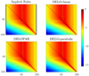Fig. 1. Values of log10|Id − JΛT|ij for i, j = 1, …, 2Ns and multiple formal solvers, with Ns = 80, NΩ = 21, and Nν = 20.

a large value of the entry |Id − JΛT|_ij, with i, j ∈ {1, ..., 2N_s}, indicates that σ_i depends strongly on σ_j. The asymmetry of the matrices is mainly due to the usage of a nonuniform spatial grid. The matrices entries show that, as expected, for τ ≤ 1 (i.e., i < 90) the solution σ depends mostly on a region in the neighborhood of τ = 1. As τ increases this effect becomes less evident and the solution depends predominantly on neighboring nodes.

4.1. Impact of spectral and angular quadratures

Figure 2 illustrates that, once a minimal resolution is guaranteed, varying the number of nodes in the spectral and angular grids N_ν and N_Ω, respectively, has a negligible effect on ρ(G). Therefore, the setting N_ν = 21 and N_Ω = 20 remains fixed in the following numerical analysis.

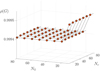Fig. 2. Spectral radius of the iteration matrix ρ(G) for the DELO-linear formal solver and the Richardson iterative method, with Ns = 40, varying NΩ and Nν. The same behavior is observed for the other iterative methods and formal solvers analyzed, as well as for different values of Ns.

4.2. Impact of the formal solver

We now present the convergence rates of various undamped (i.e., with ω = 1) iterative solvers, as a function of the number of spatial nodes for various formal solvers. The numerical results are summarized in Fig. 3. For the Richardson method (a.k.a. Λ−iteration) we observe that ρ(G)≈1, resulting in a very slow convergence. Indeed, this method is seldom used in practical applications. Moreover, we generally observe a lower convergence rates as N_s increases for all formal solvers. Among the considered formal solvers, DELOPAR shows the best convergence when combined with the Jacobi and Gauss-Seidel iterative methods. For the same iterative methods, DELOPAR is not convergent for N_s = 10, because in this case the matrix P⁻¹(Id − JΛT) has one negative eigenvalue, and thus Eq. (10) is not satisfied. A particular case is given by the DELO-parabolic, for which the Jacobi and block-Jacobi iterative methods never converge.

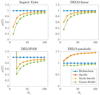Fig. 3. Spectral radius of the iteration matrix ρ(G) for multiple formal solvers and undamped iterative methods with NΩ = 20, Nν = 21, and varying Ns.

4.3. Impact of the damping parameter

We now discuss the impact of the damping parameter ω introduced in Sect. 2.3. Figure 4 reports ρ(G) for the damped methods as a function of the damping parameter ω and for multiple formal solvers. The top left panel shows that the impact of the damping parameter on the Richardson method is barely perceivable. Similarly, top right and bottom left panels indicates that the impact of the damping parameter on the Jacobi and block-Jacobi methods is not particularly pronounced. In fact, the spectral radius provided by the optimal parameter does not differ substantially from the value obtained with ω = 1. However, a quite interesting result is revealed: the Jacobi and block-Jacobi methods (at ω = 1) combined with the DELO-parabolic formal solver yield a spectral radius bigger than unity, preventing convergence. However, the use of a suitable damping parameter (ω < 0.81) enforces stability, guaranteeing convergence. An illustrative application of the damped block-Jacobi iterative method to transfer of polarized radiation is given by Janett et al. (2021). The bottom right panel confirms that the impact of the damping parameter in the SOR method is particularly effective. Indeed, a suitable choice of the damping parameter significantly reduces the spectral radius of the iteration matrix, increasing the convergence rate of the SOR method. This is consistent with the results of the previous investigations by Trujillo Bueno & Fabiani Bendicho (1995) and Trujillo Bueno & Manso Sainz (1999). We notice that the optimal damping parameter cannot be calculated with Eq. (12) for the DELO-parabolic case, since κ = ρ(G_Jac) is larger then one. Moreover, using the implicit Euler and DELOPAR formal solvers, the matrix G_Jac has few complex eigenvalues and therefore the estimate Eq. (12) is not sharp.

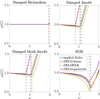Fig. 4. Spectral radius of the iteration matrix ρ(G) for multiple formal solvers and damped iterative methods with NΩ = 20, Nν = 21, Ns = 80, and varying the damping parameter ω. Vertical dashed lines represent the optimal damping parameters defined in Sect. 2.3.

Figure 5 collects the convergence rates of the damped Jacobi and SOR methods, using the optimal damping parameters ω_opt and ω_sor defined in Sect. 2.3.

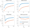Fig. 5. Spectral radius of the iteration matrix ρ(G) for multiple formal solvers and for the damped-Jacobi and SOR iterative methods with NΩ = 20, Nν = 21, and varying Ns. For the damped-Jacobi and SOR methods, we used ωopt from Eq. (11) and ωsor from Eq. (12), respectively. Since Eq. (12) cannot be applied if κ < 1, the ωsor corresponding to DELOPAR is used for the DELO-parabolic formal solver.

4.4. Impact of the collisional destruction probability

Figure 6 reports convergence rates for multiple ϵ ∈ [10⁻⁶, 1), showing that a larger ϵ corresponds to faster convergence for all the iterative methods and formal solvers under investigation. This result indicates that the numerical solution becomes easier when collision effects prevail.

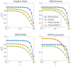Fig. 6. Spectral radius of the iteration matrix ρ(G) for multiple formal solvers and undamped iterative methods with NΩ = 20, Nν = 21, Ns = 40, and varying the collisional destruction probability ϵ.

5. Conclusions

This paper presents a fully algebraic formulation of a linear transfer problem for polarized radiation allowing for a formal analysis that aims to better understand the convergence properties of stationary iterative methods. In particular, we investigate how the convergence conditions of these methods depend on different problem and discretization settings, identifying cases where instability issues appear and exposing how to deal with them.

Numerical experiments confirm that the number of nodes in the spectral and angular grids has a negligible effect on the spectral radius of iteration matrices of various methods and, hence, on their convergence properties. By contrast, a larger number of spatial nodes leads to a reduction of convergence rates for all iterative methods and formal solvers under investigation.

In general, the use of damping parameters can both enforce stability and increase the convergence rate. Additionally, the optimal parameters described in Sect. 2.3 are indeed effective, especially in the SOR case. In the particular case, where the Jacobi and block-Jacobi methods are combined with the DELO-parabolic formal solver, the spectral radius of the iteration matrix becomes larger than unity. Hence, unless a suitable damping parameter is used, this combination is not convergent.

We remark that in this paper, we considered a specific benchmark linear radiative transfer problem. However, the presented methodology can also be applied to a wider range of settings, such as the unpolarized case, two-term atomic models including continuum contributions, 3D atmospheric models with arbitrary magnetic and bulk velocity fields, and theoretical frameworks accounting for PRD effects.

Moreover, the algebraic formulation of the transfer problem is used here exclusively as a practical tool for the convergence analysis. In the setting we have considered, the whole transfer problem is encoded in a dense linear system of size 2N_s. Different choices of the unknown vector (I, σ, or S) result in systems with different size, algebraic properties, and sparsity patterns.

However, this algebraic formulation paves the way to the application of advanced solution methods for linear (or nonlinear) systems, arising from radiative transfer applications. In particular, many state-of-the-art parallel numerical techniques can be employed, such as Krylov methods (see, e.g., Lambert et al. 2015), parallel preconditioners and multigrid acceleration (Hackbusch 2016; Saad 2003). Stationary iterative methods can also be applied as smoothers for multigrid techniques. These methods can also be applied in parallel, using available numerical libraries, which are tailored for high performance computing. In particular, Krylov methods are the subject of study of the second part of this paper series (Benedusi et al. 2021).

Acknowledgments

Special thanks are extended to E. Alsina Ballester, N. Guerreiro, and T. Simpson for particularly enriching comments on this work. The authors gratefully acknowledge the Swiss National Science Foundation (SNSF) for financial support through grant CRSII5_180238. Rolf Krause acknowledges the funding from the European High-Performance Computing Joint Undertaking (JU) under grant agreement No 955701 (project TIME-X). The JU receives support from the European Union’s Horizon 2020 research and innovation programme and Belgium, France, Germany, Switzerland.

References

Appendix A: Matrix J

The vector I ∈ ℝ^4N_sN_ΩN_ν collects all the discrete values of the Stokes parameters with the order defined by the tensor notation I ∈ ℝ^N_s × ℝ⁴ × ℝ^N_Ω × ℝ^N_ν, namely,

$$\begin{array}{cc}\hfill \mathbf{I}=& [I_1({\mathbf{r}}_1,{\mathrm{\Omega }}_1,{\nu }_1),I_1({\mathbf{r}}_1,{\mathrm{\Omega }}_1,{\nu }_2),\dots ,I_1({\mathbf{r}}_1,{\mathrm{\Omega }}_1,{\nu }_{N_{\nu }}),I_1({\mathbf{r}}_1,{\mathrm{\Omega }}_2,{\nu }_1),\dots ,I_1({\mathbf{r}}_1,{\mathrm{\Omega }}_2,{\nu }_{N_{\nu }}),\dots ,I_1({\mathbf{r}}_1,{\mathrm{\Omega }}_{N_{\mathrm{\Omega }}},{\nu }_{N_{\nu }}),I_2({\mathbf{r}}_1,{\mathrm{\Omega }}_1,{\nu }_1),\hfill \\ \hfill & \dots ,I_2({\mathbf{r}}_1,{\mathrm{\Omega }}_{N_{\mathrm{\Omega }}},{\nu }_{N_{\nu }}),\dots ,I_4({\mathbf{r}}_1,{\mathrm{\Omega }}_{N_{\mathrm{\Omega }}},{\nu }_{N_{\nu }}),I_1({\mathbf{r}}_2,{\mathrm{\Omega }}_1,{\nu }_1),\dots ,I_1({\mathbf{r}}_2,{\mathrm{\Omega }}_{N_{\mathrm{\Omega }}},{\nu }_{N_{\nu }}),\dots ,I_4{({\mathbf{r}}_{N_s},{\mathrm{\Omega }}_{N_{\mathrm{\Omega }}},{\nu }_{N_{\nu }}]}^T.\hfill \end{array}$$(A.1)

We also define the vector ${\mathbf{I}}_k\in {\mathbb{R}}^{4N_{\mathrm{\Omega }}{N}_{\nu }}$ given by

$$\begin{array}{c}\hfill {\mathbf{I}}_k={[I_1({\mathbf{r}}_k,{\mathrm{\Omega }}_1,{\nu }_1),\dots ,I_4({\mathbf{r}}_k,{\mathrm{\Omega }}_{N_{\mathrm{\Omega }}},{\nu }_{N_{\nu }})]}^T,\end{array}$$

which collects the entries of I corresponding to the spatial point r_k, such that $\mathbf{I}={\left[{\mathbf{I}}_1^T,\dots ,{\mathbf{I}}_{N_s}^T\right]}^T$.

For K = 0, 1, 2, Q = −K, …, K and k = 1, …, N_s we express (18) and (19) as

$$\begin{array}{c}\hfill {\sigma }_Q^K({\mathbf{r}}_k)=\sum _{i=1}^4\sum _{m=1}^{N_{\mathrm{\Omega }}}\sum _{p=1}^{N_{\nu }}{J}_{KQ,i}({\mathbf{r}}_k,{\mathrm{\Omega }}_m,{\nu }_p)I_i({\mathbf{r}}_k,{\mathrm{\Omega }}_m,{\nu }_p)+c_Q^K({\mathbf{r}}_k)=a_{J_u{J}_{\ell }}^{(K,Q)}({\mathbf{r}}_k){\mathbf{k}}_{-Q}^K{\mathbf{I}}_k+c_Q^K({\mathbf{r}}_k),\end{array}$$(A.2)

where

$$\begin{array}{c}\hfill J_{KQ,i}({\mathbf{r}}_k,{\mathrm{\Omega }}_m,{\nu }_p)=a_{J_u{J}_{\ell }}^{(K,Q)}({\mathbf{r}}_k){\mathbf{k}}_{-Q,N_{\nu }{N}_{\mathrm{\Omega }}(i-1)+N_{\nu }(m-1)+p}^K.\end{array}$$(A.3)

The row vector ${\mathbf{k}}_{-Q}^K\in {\mathbb{R}}^{4N_{\mathrm{\Omega }}{N}_{\nu }}$ collects the quadrature coefficients for the integral in (14) and is given by the Kronecker product

$$\begin{array}{c}\hfill {\mathbf{k}}_Q^K=\frac{1}{4\pi }{\mathit{\psi }}_Q^K\otimes \mathit{\varphi },\end{array}$$(A.4)

where ${\mathbf{\psi }}_Q^K\in {ℝ}^{4N_{\mathrm{\Omega }}}$ and ϕ ∈ ℝ^N_ν are given by

$$\begin{array}{cc}\hfill {\mathit{\psi }}_{Q,(i-1)N_{\mathrm{\Omega }}+m}^K& ={\mathcal{T}}_{Q,i}^K({\mathrm{\Omega }}_m)u_m,\text{for}i=1,\dots ,4\text{and}m=1,\dots ,N_{\mathrm{\Omega }},\hfill \\ \hfill {\mathit{\varphi }}_p& =\varphi ({\nu }_p)v_p,\text{for}p=1,\dots ,N_{\nu },\hfill \end{array}$$

and u_m and v_p are the quadrature weights of the grids ${\left\{{\mathbf{\Omega }}_m\right\}}_{m=1}^{N_{\mathrm{\Omega }}}$ and ${\left\{{\nu }_p\right\}}_{p=1}^{N_{\nu }}$, respectively.

The matrix $J\in {\mathbb{R}}^{9N_s\times 4N_s{N}_{\mathrm{\Omega }}{N}_{\nu }}$ appearing in (22) is then given by

$$J=\left[\begin{array}{ccc}\overline{J}({\mathbf{r}}_1)& & \\ & \overline{J}({\mathbf{r}}_2)& \\ & \ddots & \\ & & \overline{J}({\mathbf{r}}_{N_s})\\ \end{array}\right],\text{where}\overline{J}({\mathbf{r}}_k)=\left[\begin{array}{c}{a}_{J_u{J}_{\ell }}^{(0,0)}({\mathbf{r}}_k){\mathbf{k}}_0^0\\ a_{J_u{J}_{\ell }}^{(1,-1)}({\mathbf{r}}_k){\mathbf{k}}_1^1\\ a_{J_u{J}_{\ell }}^{(1,0)}({\mathbf{r}}_k){\mathbf{k}}_0^1\\ ⋮\\ a_{J_u{J}_{\ell }}^{(2,1)}({\mathbf{r}}_k){\mathbf{k}}_{-1}^2\\ a_{J_u{J}_{\ell }}^{(2,2)}({\mathbf{r}}_k){\mathbf{k}}_{-2}^2\\ \end{array}\right].$$

The matrix $\overline{J}({\mathbf{r}}_k)\in {\mathbb{R}}^{9\times 4N_{\mathrm{\Omega }}{N}_{\nu }}$, which collects the coefficients $a_{J_u{J}_{\ell }}^{(K,Q)}({\mathbf{r}}_k){\mathbf{k}}_{-Q}^K$ is generally dense, but it also contains zero blocks, because ${\mathcal{T}}_{Q,i}^K({\Omega }_m)$ is null for certain triples i, K, Q.

Accordingly to the structure of J, the vectors $\mathit{\sigma },\mathbf{c}\in {\mathbb{R}}^{9N_s}$ appearing in (22) are given by

$$\begin{array}{cc}& \mathbf{c}={[\stackrel{\sim }{\mathbf{c}}({\mathbf{r}}_1),\stackrel{\sim }{\mathbf{c}}({\mathbf{r}}_2),\dots ,\stackrel{\sim }{\mathbf{c}}({\mathbf{r}}_{N_s})]}^T\text{with}\stackrel{\sim }{\mathbf{c}}({\mathbf{r}}_k)=[c_0^0({\mathbf{r}}_k),c_{-1}^1({\mathbf{r}}_k),c_0^1({\mathbf{r}}_k),\dots ,c_2^2({\mathbf{r}}_k)]\in {\mathbb{R}}^9,\hfill \\ \hfill & \mathit{\sigma }={[\stackrel{\sim }{\mathit{\sigma }}({\mathbf{r}}_1),\stackrel{\sim }{\mathit{\sigma }}({\mathbf{r}}_2),\dots ,\stackrel{\sim }{\mathit{\sigma }}({\mathbf{r}}_{N_s})]}^T\text{with}\stackrel{\sim }{\mathit{\sigma }}({\mathbf{r}}_k)=[{\sigma }_0^0({\mathbf{r}}_k),{\sigma }_{-1}^1({\mathbf{r}}_k),{\sigma }_0^1({\mathbf{r}}_k),\dots ,{\sigma }_2^2({\mathbf{r}}_k)]\in {\mathbb{R}}^9.\hfill \end{array}$$

For completeness, we express the entries of the matrix J in term of the coefficient appearing in (19), namely,

$$J_{KQ,i}({\mathbf{r}}_k,{\mathrm{\Omega }}_m,{\nu }_p)=J_{l{l}^{\prime }},\text{with}l=9(k-1)+K(K+1)+Q+1\text{and}{l}^{\prime }=4N_{\mathrm{\Omega }}{N}_{\nu }(k-1)+N_{\mathrm{\Omega }}{N}_{\nu }(i-1)+N_{\nu }(m-1)+p.$$

Appendix B: Matrix T

The vector S ∈ ℝ^4N_sN_Ω collects all the discrete values of the source function vector with the order defined by the tensor notation S ∈ ℝ^N_s × ℝ⁴ × ℝ^N_Ω, namely,

$$\begin{array}{c}\hfill \mathbf{S}={[S_1({\mathbf{r}}_1,{\mathrm{\Omega }}_1),S_1({\mathbf{r}}_1,{\mathrm{\Omega }}_2),\dots ,S_1({\mathbf{r}}_1,{\mathrm{\Omega }}_{N_{\mathrm{\Omega }}}),S_2({\mathbf{r}}_1,{\mathrm{\Omega }}_1),\dots ,S_2({\mathbf{r}}_1,{\mathrm{\Omega }}_{N_{\mathrm{\Omega }}}),\dots ,S_4({\mathbf{r}}_1,{\mathrm{\Omega }}_{N_{\mathrm{\Omega }}}),S_1({\mathbf{r}}_2,{\mathrm{\Omega }}_1),\dots ,S_4({\mathbf{r}}_{N_s},{\mathrm{\Omega }}_{N_{\mathrm{\Omega }}})]}^T.\end{array}$$

We also define the auxiliary vector ${\mathbf{w}}_i(\mathrm{\Omega })\in {\mathbb{R}}^9$ given by

$$\begin{array}{c}\hfill {\mathbf{w}}_i(\mathrm{\Omega })=[w_{J_u{J}_{\ell }}^{(0)}{\mathcal{T}}_0^0(i,\mathrm{\Omega }),w_{J_u{J}_{\ell }}^{(1)}{\mathcal{T}}_{-1}^1(i,\mathrm{\Omega }),w_{J_u{J}_{\ell }}^{(1)}{\mathcal{T}}_0^1(i,\mathrm{\Omega }),\dots ,w_{J_u{J}_{\ell }}^{(2)}{\mathcal{T}}_1^2(i,\mathrm{\Omega }),w_{J_u{J}_{\ell }}^{(2)}{\mathcal{T}}_2^2(i,\mathrm{\Omega })].\end{array}$$

The matrix $T\in {\mathbb{R}}^{4N_s{N}_{\mathrm{\Omega }}\times 9N_s}$ appearing in (23) is then given by

$$T=\left[\begin{array}{ccc}W& & \\ & W& \\ & \ddots & \\ & & W\\ \end{array}\right],\text{where}W=\left[\begin{array}{c}{\mathbf{w}}_1({\mathrm{\Omega }}_1)\\ {\mathbf{w}}_1({\mathrm{\Omega }}_2)\\ ⋮\\ {\mathbf{w}}_1({\mathrm{\Omega }}_{N_{\mathrm{\Omega }}})\\ {\mathbf{w}}_2({\mathrm{\Omega }}_1)\\ ⋮\\ {\mathbf{w}}_4({\mathrm{\Omega }}_{N_{\mathrm{\Omega }}})\\ \end{array}\right].$$

The matrix $W\in {\mathbb{R}}^{4N_{\mathrm{\Omega }}\times 9}$ is generally dense and the matrix T is also given by the Kronecker product $T=I{d}_{N_s}\otimes W$, where $I{d}_{N_s}$ is the identity matrix of size N_s.

Appendix C: Matrix Λ

For the sake of clarity, the implicit Euler method is used to integrate the transfer equation (15). However, the same analysis can be generalized to any formal solver. For simplicity, we consider the 1D plane-parallel cylindrical symmetric atmospheric model used in Section 4.

The angular dependence of the problem is encoded by the scalar μ = cos(θ) with the corresponding discrete grid

$$\begin{array}{c}\hfill -1\le {\mu }_1<{\mu }_2<\dots <{\mu }_{N_{\mathrm{\Omega }}-1}<{\mu }_{N_{\mathrm{\Omega }}}\le 1.\end{array}$$

The spatial dependence of the problem is encoded either by the scalar s with the corresponding discrete grid ${\left\{s_k\right\}}_{k=1}^{N_s}$ or by the scaled line-center frequency optical depth τ with the corresponding discrete grid ${\left\{{\tau }_k\right\}}_{k=1}^{N_s}$. The relation between the two spatial variables is described by

$$\varphi (\nu )\mathrm{d}\tau =-\eta (s,\nu )\mathrm{d}s$$

and the transfer equation (15) can then be expressed as

$$\begin{array}{c}\hfill \frac{\mu }{\varphi (\nu )}\frac{\mathrm{d}}{\mathrm{d}\tau }{I}_i(\tau ,\mu ,\nu )=I_i(\tau ,\mu ,\nu )-S_i(\tau ,\mu ).\end{array}$$(C.1)

Applying the implicit Euler method to (C.1) for i = 1, …, 4, we obtain, for incoming and outgoing directions respectively

$$\begin{array}{cc}\hfill I_i({\tau }_{k+1},\mu ,\nu )& =\frac{I_i({\tau }_k,\mu ,\nu )+\mathrm{\Delta }{\tau }_k(\mu ,\nu )S_i({\tau }_{k+1},\mu )}{1+\mathrm{\Delta }{\tau }_k(\mu ,\nu )},\text{for}\mu <0\text{and}k=1,\dots ,N_s-1,\hfill \end{array}$$(C.2)

$$\begin{array}{cc}\hfill I_i({\tau }_{k-1},\mu ,\nu )& =\frac{I_i({\tau }_k,\mu ,\nu )+\mathrm{\Delta }{\tau }_{k-1}(\mu ,\nu )S_i({\tau }_{k-1},\mu )}{1+\mathrm{\Delta }{\tau }_{k-1}(\mu ,\nu )},\text{for}\mu >0\text{and}k=N_s,N_s-1,\dots ,2,\hfill \end{array}$$(C.3)

where

$$\begin{array}{c}\hfill \mathrm{\Delta }{\tau }_k(\mu ,\nu )=\frac{\varphi (\nu )}{|\mu |}|{\tau }_{k+1}-{\tau }_k|.\end{array}$$

We notice that different Stokes parameters, directions and frequencies are decoupled in the transfer equation (15) and, consequently, in the discrete counterparts (C.2) and (C.3). Providing the initial conditions $I_i({\tau }_1,\mu ,\nu )=I_i^{\text{in}}(\mu ,\nu )$ for μ < 0 and $I_i({\tau }_{N_s},\mu ,\nu )=I_i^{\text{out}}(\mu ,\nu )$ for μ > 0, we recursively apply (C.2) and (C.3) and obtain

$$\begin{array}{cc}\hfill I_i({\tau }_k,\mu ,\nu )& =f_k(\mu ,\nu )I_i^{\text{in}}(\mu ,\nu )+{\displaystyle \sum _{j=2}^k{f}_{k,j}(\mu ,\nu )S_i({\tau }_j,\mu )\text{for}\mu <0\text{and}k=2,\dots ,N_s,}\hfill \end{array}$$(C.4)

$$\begin{array}{cc}\hfill I_i({\tau }_k,\mu ,\nu )& =h_k(\mu ,\nu )I_i^{\text{out}}(\mu ,\nu )+{\displaystyle \sum _{j=k}^{N_s-1}{h}_{k,j}(\mu ,\nu )S_i({\tau }_j,\mu )\text{for}\mu >0\text{and}k=1,\dots ,N_s-1,}\hfill \end{array}$$(C.5)

with

$$\begin{array}{cc}\hfill f_{k,j}(\mu ,\nu )& =\frac{\mathrm{\Delta }{\tau }_{j-1}(\mu ,\nu )}{{\prod }_{l=j}^{k}1+\mathrm{\Delta }{\tau }_{l-1}(\mu ,\nu )}\text{and}{f}_k(\mu ,\nu )=\frac{1}{{\prod }_{l=1}^{k-1}1+\mathrm{\Delta }{\tau }_l(\mu ,\nu )},\hfill \end{array}$$(C.6)

References

- Alsina Ballester, E., Belluzzi, L., & Trujillo Bueno, J. 2017, ApJ, 836, 6 [Google Scholar]
- Alsina Ballester, E., Belluzzi, L., & Trujillo Bueno, J. 2018, ApJ, 854, 150 [Google Scholar]
- Belluzzi, L., & Trujillo Bueno, J. 2014, A&A, 564, A16 [NASA ADS] [CrossRef] [EDP Sciences] [Google Scholar]
- Benedusi, P., Janett, G., Belluzzi, L., & Krause, R. 2021, A&A, 655, A88 [NASA ADS] [CrossRef] [EDP Sciences] [Google Scholar]
- del Pino Alemán, T., Trujillo Bueno, J., Casini, R., & Manso Sainz, R. 2020, ApJ, 891, 91 [CrossRef] [Google Scholar]
- Hackbusch, W. 2016, in Iterative Solution of Large Sparse Systems of Equations, 2nd edn. (Springer), Appl. Math. Sci., 95 [CrossRef] [Google Scholar]
- Hageman, L. A., & Young, D. M. 1981, Applied Iterative Methods (New York, NY, USA: Academic) [Google Scholar]
- Hubeny, I. 2003, in Stellar Atmosphere Modeling, 288, 17 [NASA ADS] [Google Scholar]
- Janett, G., & Paganini, A. 2018, ApJ, 857, 91 [Google Scholar]
- Janett, G., Carlin, E. S., Steiner, O., & Belluzzi, L. 2017a, ApJ, 840, 107 [NASA ADS] [CrossRef] [Google Scholar]
- Janett, G., Steiner, O., & Belluzzi, L. 2017b, ApJ, 845, 104 [Google Scholar]
- Janett, G., Ballester, E. A., Guerreiro, N., et al. 2021, A&A, 655, A13 [NASA ADS] [CrossRef] [EDP Sciences] [Google Scholar]
- Klein, R. I., Castor, J. I., Greenbaum, A., Taylor, D., & Dykema, P. G. 1989, J. Quant. Spectr. Rad. Transf., 41, 199 [NASA ADS] [CrossRef] [Google Scholar]
- Lambert, J., Josselin, E., Ryde, N., & Faure, A. 2015, A&A, 580, A50 [NASA ADS] [CrossRef] [EDP Sciences] [Google Scholar]
- Lambert, J., Paletou, F., Josselin, E., & Glorian, J.-M. 2016, Eur. J. Phys., 37, 015603 [Google Scholar]
- Landi Degl’Innocenti, E., & Landolfi, M. 2004, in Polarization in Spectral Lines, (Dordrecht: Kluwer Academic Publishers), Astrophys. Space Sci. Lib., 307 [Google Scholar]
- Olson, G. L., Auer, L. H., & Buchler, J. R. 1986, J. Quant. Spectr. Rad. Transf., 35, 431 [Google Scholar]
- Paletou, F., & Auer, L. H. 1995, A&A, 297, 771 [NASA ADS] [Google Scholar]
- Quarteroni, A., Sacco, R., & Saleri, F. 2010, Numerical Mathematics (Springer Science& Business Media), 37 [Google Scholar]
- Rybicki, G. B., & Hummer, D. G. 1991, A&A, 245, 171 [NASA ADS] [Google Scholar]
- Saad, Y. 2003, Iterative Methods for Sparse Linear Systems (SIAM) [Google Scholar]
- Sampoorna, M., & Trujillo Bueno, J. 2010, ApJ, 712, 1331 [NASA ADS] [CrossRef] [Google Scholar]
- Sampoorna, M., Nagendra, K. N., & Stenflo, J. O. 2017, ApJ, 844, 97 [NASA ADS] [CrossRef] [Google Scholar]
- Trujillo Bueno, J., & Fabiani Bendicho, P. 1995, ApJ, 455, 646 [NASA ADS] [CrossRef] [Google Scholar]
- Trujillo Bueno, J., & Landi Degl’Innocenti, E. 1996, Sol. Phys., 164, 135 [NASA ADS] [CrossRef] [Google Scholar]
- Trujillo Bueno, J., & Manso Sainz, R. 1999, ApJ, 516, 436 [NASA ADS] [CrossRef] [Google Scholar]