| Issue |
A&A
Volume 655, November 2021
|
|
|---|---|---|
| Article Number | A68 | |
| Number of page(s) | 11 | |
| Section | Galactic structure, stellar clusters and populations | |
| DOI | https://doi.org/10.1051/0004-6361/202140475 | |
| Published online | 19 November 2021 | |
FEDReD
III. Unraveling the 3D structure of Vela⋆
1
GEPI, Observatoire de Paris, CNRS, Université Paris Diderot, 5 place Jules Janssen, 92190 Meudon, France
e-mail: This email address is being protected from spambots. You need JavaScript enabled to view it.
2
Univ. Grenoble Alpes, CNRS, IPAG, 38000 Grenoble, France
Received:
1
February
2021
Accepted:
16
August
2021
Abstract
Context. The Vela complex is a region of the sky that gathers several stellar and interstellar structures in a few hundred square degrees.
Aims.Gaia data now allow us to obtain a 3D view of the Vela interstellar structures through the dust extinction.
Methods. We used the FEDReD (Field Extinction-Distance Relation Deconvolver) algorithm on near-infrared 2MASS data, cross-matched with the Gaia DR2 catalogue, to obtain a 3D cube of extinction density. We applied the FellWalker algorithm to this cube to locate clumps and dense structures.
Results. We analysed 18 million stars over 450 deg2 to obtain the extinction density of the Vela complex from 0.5 to 8 kpc at ℓ ∈ [250° ,280° ] and b ∈ [ − 10° ,5° ]. This cube reveals the complete morphology of known structures and relations between them. In particular, we show that the Vela Molecular Ridge is more likely composed of three substructures instead of four, as suggested by the 2D densities. These substructures form the shell of a large cavity. This cavity is visually aligned with the Vela supernova remnant but located at a greater distance. We provide a catalogue of location, distance, size, and total dust content of Interstellar Medium (ISM).
Key words: dust / extinction / ISM: structure / ISM: individual objects: Vela Molecular Ridge
Datacube is only available at the CDS via anonymous ftp to cdsarc.u-strasbg.fr (130.79.128.5) or via http://cdsarc.u-strasbg.fr/viz-bin/cat/J/A+A/655/A68
© C. Hottier et al. 2021
 Open Access article, published by EDP Sciences, under the terms of the Creative Commons Attribution License (https://creativecommons.org/licenses/by/4.0), which permits unrestricted use, distribution, and reproduction in any medium, provided the original work is properly cited.
1. Introduction
A large number of structures are known towards the Vela constellation. A view from the Improved Reprocessing of the IRAS Survey (Miville-Deschênes & Lagache 2005, IRIS) of this sky area is displayed in Fig. 1. This is the Vela complex. All of its structures reside in the region defined by 240° ≤ ℓ ≤ 280° and 6° ≤ b ≤ −20° (Pettersson 2008). As stellar structures, we count several OB associations as well as R associations (Pettersson 2008). However, the Vela complex also presents several large interstellar structures.
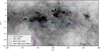 |
Fig. 1. View of the Vela complex at 60 μm with the Improved Reprocessing of the IRAS Survey (IRIS Miville-Deschênes & Lagache 2005). The colour map is on a logarithmic scale. We overlay the approximate location of the main Vela substructures discussed in the text. |
The Gum nebula (Gum 1952) is the largest structure of the area (Pettersson 2008). It is a ring shell structure with an angular diameter of 34° centred at (ℓ,b) =(262°, −3°) (Reynoso & Dubner 1997) at a distance of 450 pc. The nebula is expanding and shares this expansion with the cometary globules (Woermann et al. 2001), which are a set of dark clouds with tails pointing to the centre of the Gum nebula (Pettersson 2008).
The Vela surpernova remnant (VSNR) structure is located at (ℓ,b) = (263.9°, −3.3°), centred on the Vela Pulsar, PSR B0-833-45, with an angular diameter of ≈8° (Pettersson 2008). The estimated distance varies from 250 pc to 600 pc (Cha et al. 1999, and references therein).
The IRAS Vela shell (hereafter IVS) is a ring shell first noticed in IRAS data by Sahu (1992). It is centred at (ℓ,b) = (263°, −7°) at the distance of 450 pc (Pettersson 2008). This shell is related to the Vela OB2 association and may have a common progenitor and may share their histories (Cantat-Gaudin et al. 2019, and references therein).
It is canonically accepted that all these structures are quite close to the Sun. The Vela complex nevertheless also presents a large ridge in the background. It was first noticed in the CO Survey (Dame et al. 1987; May et al. 1988) and named Vela Molecular Ridge (VMR) by Murphy & May (1991). This structure can be split into four parts, A, B, C, and D, according to CO peaks. Liseau et al. (1992) estimated the distances to VMR A, C, and D at 0.7 ± 0.2 kpc and VMR B at 2 kpc using infrared photometry, which could imply that VMR B is not related to the A, C, and D parts. More recently, Massi et al. (2019) used a stellar parallax from Gaia DR2 (Gaia Collaboration 2018) to estimate the VMR C distances farther at D = 0.95 ± 0.05 kpc.
As shown by the previous paragraph, the Vela region has been studied through several markers and techniques, but the extinction component, especially in 3D, is poorly exploited compared to other tracers. Franco (2012) analysed the interstellar reddening in six distinct areas using photometry to study the largest structures of the Vela complex, but not the densest parts of the complex.
On the other hand, there are some 3D extinction maps, but some of them are focused on other regions, such as Chen et al. (2013) or Schultheis et al. (2014), which compare photometric surveys to the Besançon model (Robin et al. 2012) to study the Galactic bulge. Sale et al. (2014) and Green et al. (2018) both used a Bayesian approach, respectively, on the IPHAS survey and on Pan-STARRS and 2MASS, to derive extinctions. Rezaei Kh et al. (2018) analysed the APOGEE survey with a non-parametric 3D inversion to obtain the dust density. However, these three techniques used northern sky surveys, so they are not able to reach Vela.
There are also some 3D extinction maps that cover the Vela direction. Capitanio et al. (2017) and Lallement et al. (2019) applied the 3D inversion technique of Vergely et al. (2001) on composite dust proxies using, respectively, the Gaia DR1 parallaxes and the 2MASS cross-match with Gaia DR2. Chen et al. (2019) used a random forest algorithm on a dataset built with Gaia DR2, WISE, and 2MASS to compute the extinction density. Hottier et al. (2020) analysed 2MASS and Gaia DR2 data with the FEDReD algorithm (Babusiaux et al. 2020) and derived the extinction density in the Galactic plane.
However, as far as we know, there is no study focussing on the 3D extinction structure of the Vela complex. In a previous work (Hottier et al. 2020), we noticed that the Vela complex presents large structures that reach distances up to 5 kpc. We also discussed the possibility that the Vela complex could belong to the local arm in Hottier et al. (2020). This belonging seems to be confirmed by the spiral arm locations found by Khoperskov et al. (2020). Studying the Vela complex could therefore give us the opportunity to study a spiral arm viewed from the inside.
In this work, we used FEDReD to probe the 3D extinction density distribution towards Vela. In Sect. 2, we present the analysed dataset. Section 3 sums up the FEDReD algorithm and develops the differences from Hottier et al. (2020). In Sect. 4 we present the method of clump extraction. Section 5 describes and analyses the 3D density map and the clumps and cavities extracted from it.
2. Data
In this study, we used the infrared photometry in bands J, H, and K from the 2MASS survey (Skrutskie et al. 2006) and we combined them with the photometry in bands G, GBP, and GRP and the astrometry from the Gaia DR2 (Gaia Collaboration 2018). We used the same methodology as Hottier et al. (2020) to filter and merge data of these surveys, so we simply give a brief review of them here.
We used the 2MASS near-infrared photometry as principal data; hence, our dataset completeness will be the 2MASS one. In practice, every star included in our dataset has ph_qual≥D in all three J, H, and K bands. Once we selected the stars in 2MASS, we used the Marrese et al. (2019) cross-match to potentially add Gaia DR2 parallaxes and photometry.
To filter the Gaia photometry (Evans et al. 2018), we do not use GBP and GRP when phot_bp_rp_excess_factor > 1.3 + 0.06 × (GBP − GRP)2 and GBP > 18 according to Evans et al. (2018) and Arenou et al. (2018). For the astrometric information (Lindegren et al. 2018), we used Eq. (1) of Arenou et al. (2018), we corrected the parallax zero point of −0.03 mas, and we did not use the parallax when ϖ + 3 × σϖ < 0 to remove spurious astrometric solutions.
3. Extinction map with FEDReD
To analyse this dataset, we used the FEDReD algorithm. The entire algorithm description as well as tests on mock and observed data are presented in Babusiaux et al. (2020). Thus, we simply explain the main steps of the algorithm and differences from Hottier et al. (2020) briefly.
3.1. Field-of-view analysis
FEDReD analyses photometric and astrometric data, field of view by field of view, and infers both the evolution of the extinction as a function of distance and the stellar density distribution. To do so, it works in two steps.
The first step is the processing, for each star, of the likelihood of this observed star being at the distance D with extinction A0 (extinction at 550 nm) P(O∣A0,D). This distribution is processed by comparing the apparent photometry of the stars to an empirical HR diagram built from 2MASS and Gaia DR2 (see Babusiaux et al. 2020, Sect. 3.1, for details), it also uses parallax information when it is available.
Once the likelihood of each star is computed, FEDReD applies a Bayesian deconvolution to obtain the joint distribution of extinction and distances P(A0,D). This deconvolution also takes into account the completeness of the field of view, which is estimated from the observed near-infrared photometry distribution.
To initialise this deconvolution, we used two simple priors. The prior on the distance distribution is a square law of the distance, corresponding to the cone effect. Concerning the extinction given the distances, P(A0∣D), we used a uniform distribution (contrary to Hottier et al. 2020).
From the joint distribution of extinction and distance, FEDReD generates Monte-Carlo Solutions (MCSs) of the increasing relation A0(D) drawn following the probability distribution P(A0,D). As red clump stars are the ones providing the strongest constraints on the distance and extinction, we restricted our results to the distance interval [Dmin, Dmax] where red clump stars are observed by 2MASS; that is, the distance at which a red clump star saturates (Dmin) or is fainter than the completeness limit (Dmax). Unlike Hottier et al. (2020), this distance interval restriction is also used within the algorithm determining the A0(D) and not just in the post-processing. At the end of this process, we obtain 1000 MCSs by field of view.
3.2. Merging fields of view into extinction cubes
The fields of view are 0.38° wide in longitude and latitude, and the centres are spaced by 0.38° in latitude and longitude. Therefore, each field of view overlaps its first neighbour (top, bottom, left, and right) by half of its angular surface, and it overlaps its second neighbour (four diagonals) by the quarter of its angular surface. This means that each star is inside three different fields of view, which allows us a good continuity between fields of view.
To merge results from each field of view into a consistent extinction cube, we used the exact same algorithm as in Hottier et al. (2020). Firstly, we iteratively cleaned the MCS samples of each field of view using neighbour fields’ MCS envelopes as upper and lower limits. The convergence of this process is provided by the overlapping of fields. Secondly, we randomly drew one MCS per field of view (inside their respective clean pools) to obtain a relation between the extinction A0 and the distance D for each field of view. Then, at each distance bin, we smoothed the extinction value using the eight neighbour fields of view to obtain the extinction cube. We randomly drew 100 of these cubes. Finally, we used a constrained cubic spline fit (Ng & Maechler 2007) to obtain the median relation of extinction as a function of distance of each field of view. These relations were then decumulated and normalised by the distance width of bins to obtain the extinction density a0 in each voxel of the cube.
3.3. Extinction uncertainty
As in Hottier et al. (2020), we also computed the uncertainty of our extinction and extinction density cubes. Concerning the extinction A0, we used the sample of MCSs after the cleaning process by the neighbour envelope to obtain the maximum and minimum values of extinction at each distance bin (A0min(D) and A0max(D)).
To estimate the extinction density uncertainty, we used the exact same algorithm explained in Sect. 3.2 but on a bootstrapped MCS sample instead. We build 100 bootstrap-merged cubes, and we computed the standard deviation of extinction density a0 for each voxel to obtain the uncertainty on the extinction density. As discussed in Hottier et al. (2020) (Sect. 5.1), this uncertainty map mostly represents the sampling error, and it underestimates the true uncertainty of our results.
4. Clump extraction
To obtain the distance, shape, and size of extinction density clumps, we interpolated our data cube on a regular Galactic cartesian grid1 with a voxel size of 10 pc. Using this new interpolated cube, we first tried to process the iso-surface density to locate clumps. This allowed us to spatially constrain some clumps, but it required very sensitive settings for each clump we looked for. Moreover, this technique has difficulty resolving distinct clumps, and local peaks can hide the true shape and size of a clump.
Dendograms have already been used to extract clumps and molecular clouds (Goodman et al. 2009; Chen et al. 2019). This algorithm uses a hierarchical tree to segregate structures, showing relations between each clump. To do so, it only uses the local value of pixels and links voxels with their neighbours if values are compatible. But as we work with a density cube processed by line of sight, the extinction density can leak to greater distances and create some Fingers-of-God structures.
To avoid the extraction of structures only dominated by the Fingers-of-God effect, we used the FellWalker algorithm2 (Berry 2015), which identifies clumps by analysing the local gradient. In a few words, this algorithm ‘walks’ through the entire volume, voxel by voxel. To choose the next voxel, it always chooses the steepest path. When it reaches a local maximum, it checks nearby for a higher point (in order to avoid extrema due to noise). If this higher point exists, the algorithm ‘jumps’ and so on. If a higher spot does not exist, the algorithm has just reached the top of a new clump. When the entire volume is mapped, the algorithm checks if clumps can be merged. Finally, it can re-assign a voxel to the most common clump around it.
As the Finger-of-God effect also impacts the gradient of extinction density, the FellWalker algorithm is also impacted. While a minimum value-based algorithm (such as dendogram) just wipes out low-extinction structures to avoid elongations, the FellWalker algorithm can set up both a minimal value and a minimum gradient to mitigate the extraction of the Finger-of-God effect when looking for the edge of clumps, without missing the ones with low values of extinction. Nevertheless, the clump segregation depends on the parameter settings of the algorithm.
With this in mind, we manually tuned the parameters of the algorithm in order to avoid elongations and extract parts of the VMR. The minimum extinction density to be a part of a clump was 3 mag kpc−1. The size of the maximum jump was set to 4 voxels, which corresponds to 0.04 kpc. The minimum initial density variation was 0.5 mag kpc−1 from one voxel to another. Two clumps may be merged if the depth of the col between them was smaller than 3 mag kpc−1. The clump outline process was done with a 4 -voxel cube. Finally, we removed clumps containing only one or two voxels as those were just high extinction density spots induced by the decumulation process.
4.1. Processing clump parameters
The result of the FellWalker algorithm is a 3D mask for each clump. From this mask, we directly obtained angular and distance bounds of clumps, as well as the volumes of the clumps. To obtain the centre of a clump, we computed the barycentric position using the extinction density as the weight.
In order to estimate the total dust content Ac of a clump, we had to integrate the extinction density a0 over the volume of the clump:
 (1)
(1)
 (2)
(2)
If we discretise the equation, we obtain
 (3)
(3)
with i the ith voxel in the clumps; li, bi, and di the position of the voxel; a0i the extinction density in this voxel; and δdi the distance width of the voxel. As these voxels follow the cube we obtained by merging the fields of view, δli and δbi are constant over the cube δl = δb = 0.18°. In practice, as we looked for clumps in a regular cartesian cube, we used Eq. (1) in cartesian referential frame with dV = (0.01 kpc)3 and a0 the value of extinction density in each voxel. We note that these Ac can be used to estimate the masses of clumps, following the method described in Chen et al. (2020).
Some of the clumps are located on the edge of our extinction cube. We mark them as ‘not full’, and their estimated extinction is only a lower estimate, while their distance only corresponds to what we observe in our extinction cube.
4.2. Uncertainties on the parameters
To estimate the uncertainty on each parameter, we used the random cubes that we built to compute the density uncertainty. We applied the same FellWalker algorithm to them with the same parameters. We cross-identified clumps from their barycentric position and we estimated each parameter uncertainty using their standard deviation.
We kept, in the final catalogue, clumps that are detected in at least 99% of the bootstraps. Indeed, some large clumps are identified as several small ones in some bootstraps, preventing the use of a 100% threshold.
4.3. Extracting cavities
We also used the FellWalker algorithm to spatially constrain density cavities. As this algorithm is designed to search peaks rather than valleys, we inverted the values of the density cube following this equation: max(a0(l, b, d)) − a0(l, b, d). The cavities in the ‘inverted’ data cube appear more as a plateau than as a mountain, so we did not use the minimum steepness parameter. The minimum value parameter was set in order to map the area of the original cube with extinction below 0.5 mag. As for the clump extraction, we set the maximum jump to 4 voxels.
Inverting the data cube implies that every area without extinction was detected as a cavity, so areas above and below the complex are considered as many little cavities that merge into a single one during the merging process. Moreover, the shell of cavities that we can see by eye are porous, which leads them to be merged with the clean empty part below and above the complex. To avoid this phenomenon, we clean our cavity sample before the merging step. To do so, we removed the cavities with median voxel values inferior to 0.1 mag kpc−1 from the sample. Then, we merge the cavities with a col height threshold at 0.03 mag kpc−1.
Finally, we removed cavities from the edge of our field of view. If a structure is detected on the edge, it is undoubtedly a clump. However, in the case of cavity detection, we are looking for an area with low-extinction density. In the case of cavity inside our data cube, we can ensure that this area is really surrounded by an extinction shell, while a cavity on the edge of the cube can be completely open.
With regard to clumps, we also processed uncertainty on cavities parameters, but due to the large volume of the cavities and the thin shell around them, the tuning of the parameters were very sensitive. This implies that we did not recover cavities in bootstrap as often as we did for clumps. Thus, in order to provide uncertainties, we lowered the threshold to 50% to keep cavities in final our catalogue.
5. Results
We split our dataset of 18 028 023 stars into 12 403 fields of view. Each field of view is a square of 0.38° in Galactic latitudes and longitudes, with l ∈ [250° ,280° ] and b ∈ [ − 10° ,5° ].
5.1. Extinction column
In Fig. 2, we present a view of the cumulative extinction A0 of the Vela complex up to 5 kpc, roughly the distance limit of Vela complex noticed by Hottier et al. (2020), with the same boundaries as in Fig. 1. We also overplotted the main structures of Vela.
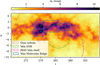 |
Fig. 2. View of the Vela complex in extinction A0 using the cumulative extinction over a distance of 5 kpc. |
The VMR appears to be the strongest extinction structure of the entire complex and is approximately located at 260° ≤ ℓ ≤ 272° and −4° ≤ b ≤ 3°. While the overall shape of the VMR is quite similar to the IRAS view shown in Fig. 1, it differs in the details, as the strongest emissions at 60 μm do not coincide with the areas with the strongest cumulative extinction. As in Fig. 1, the IVS is very faint; however, using a visual guide, it is still visible as a diffuse filament. On the other hand, due to the relatively small area covered by our study, the Gum nebula footprint cannot be distinguished.
5.2. Extinction density towards Vela
In Fig. 3, we present the extinction density a0 cut along constant Galactic latitudes. Figure 4 shows views of the extinction density at several distances. We also add the contours of clumps that we segmented with the FellWalker algorithm to those two figures.
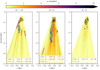 |
Fig. 3. Extinction density a0 at different Galactic latitudes b. x and y represent galactic coordinates, the Sun is at (0, 0) and the Galactic centre direction is to the right. We also add the contour of the clumps, their parameters being presented in Table 1. |
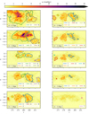 |
Fig. 4. Extinction density a0 of the Vela complex at several distances obtained with FEDReD. The contours of each clump segmented by the FellWalker algorithm is represented with lines. |
We do not provide the extinction density close to the Sun in either figure because of the red clump visibility criterion (see Sect. 3.1). To see the nearby Gum Nebula and the VSNR, we used the Lallement et al. (2019) extinction cube instead. They used the same data as this work (2MASS and Gaia DR2), restricted to stars with relative error on the parallax less than 20%, and they applied the same extinction law (see Appendix A for a more detailed comparison). In Fig. 5, we plot the extinction density that they obtained at the canonical distance of the Gum Nebula and VSNR. Indeed, at D = 0.25 kpc we saw a shell the size of the VSNR. We also see a large shell that seems to correspond to the Gum Nebula at D = 0.25 kpc, whereas we cannot distinguish any footprint at D = 0.45 kpc. This could mean that the Gum Nebula is closer than usually indicated in the literature.
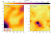 |
Fig. 5. Extinction density of the Vela complex at the distance D = 0.25 kpc and D = 0.45 kpc obtained with the Lallement et al. (2019) cube. The canonical size and location of Vela SNR and Gum Nebula (Pettersson 2008) are sketched. |
5.3. VMR and clumps
The FellWalker algorithm found 14 clumps. Table 1 presents their parameters. We identify them by a simple integer id according to their volumes. We visually identify clumps to the VMR parts (column notes of Table 1).
Density clumps found by the FellWalker algorithm.
The VMR C (clump 3) goes beyond the edge of our extinction cube, but we can see that we detect the main part of it. It begins at D = 0.5 kpc and its barycenter is at D = 0.9 ± 0.09 kpc, which is consistent with the Liseau et al. (1992) estimation at 0.7 ± 0.2 kpc. This distance is also inside the confidence interval of Massi et al. (2019) (0.950 ± 0.050 kpc), and our distance interval contains every molecular distance of Zucker et al. (2020), labelled VMRC, which range from 0.86 to 0.97 kpc. However, VMR C is very large; its longitude footprint goes from ℓ = 256° to more than ℓ = 280°, and its maximum distance reaches D = 1.6 kpc.
VMR D (clump 1), the biggest in this study, is farther than VMR C. Its barycenter is at D = 1.9 ± 0.4 kpc, and its front part is at D = 0.75 kpc, while Liseau et al. (1992) only see the front part of it and estimate VMR C, D, and A to be roughly at the same distance of 0.7 ± 0.2 kpc.
Concerning VMR A and VMR B, they are identified as a unique clump (clump 2)3. The reason why this clump is split into two pieces in the literature is the overlapping with VMR C in the foreground, which induces a projection effect. Nevertheless, VMR A is one of the biggest clumps of the Vela region, and it seems to be related to VMR C and VMR D at high distances (D > 1.2 kpc), where they form a shell (see Sect. 5.4). We can also note that this clump contains the molecular cloud RCW 38, which was located at D = 1.6 kpc by Zucker et al. (2020).
Clump 7 corresponds to the RCW 19 object (Rodgers et al. 1960), also called GUM 10 (Gum 1955). We locate it at D = 3.8 ± 0.09 kpc, which is farther than the determination D = 3.0 ± 0.3 kpc of Russeil (2003).
As far as we know, the other clumps have not yet been identified and named. Clump 8 is a large clump, and it is bigger than what we process as it goes beyond the edge of our extinction cube. Clump 6 presents a relatively high extinction density and reasonable apparent angle, but it is barely visible in the column view (Fig. 2) because it is overlapped by VMR D.
5.4. Cavities
The FellWalker algorithm found nine cavities. As for clumps, we identify them by a simple integer ID sorted by volume. We represent the contour of these cavities in distance views in Fig. 6.
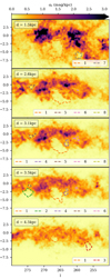 |
Fig. 6. Extinction density a0 of the Vela complex at several distances obtained with FEDReD. The lines represent the contours of the cavities we extracted with the FellWalker algorithm (parameters on Table 2). |
The biggest one (cavity 1) is centred on (ℓ,b) = (266.1°, −3.1°). It is very visible in IRAS data (Fig. 1) and on the cumulated extinction view (Fig. 2). Its angular location fits the VSNR angular location, but the centre of this cavity is at D = 3.1 ± 0.35 kpc and its closest ‘wall’ is at D = 1.2 kpc, behind the foreground part of VMR C (clump 3), and its shell is composed of all the VMR parts. On the other hand, VSNR is at 0.25 kpc, with an upper limit at 0.49 kpc (Cha et al. 1999), in the foreground of the VMR. We show its local extinction fingerprint in Fig. 5. Thus, it appears that this shell, described in the 2D views as VSNR, visible in infrared and in the extinction column, is actually composed of two distinct structures physically separated by VMR C.
As is the case for Cavity 1, Cavities 2 and 3 are under the main extinction density of the galactic plane, and their low latitude shells are very thin. While the others are located inside the galactic plane. So far, we have not found the origins of these cavities.
6. Conclusion
We used the FEDReD algorithm to analyse photometry and parallax from 2MASS and Gaia DR2 of stars in the Vela complex direction. This provided us with the distribution of the extinction density in 3D. Consequently, we were able to obtain the distance and the 3D shape of known structures of this area.
For this purpose, we applied the FellWalker algorithm, which produced very good results when applied to extracting clumps. However it turns out not to be the best designed tool to extract cavities as it requires a very specific tuning. For further investigation on cavities, we recommend using or developing other approaches, although we have not found a better one so far.
Nevertheless, we managed to spatially measure 14 dense extinction clouds (Table 1) and nine cavities (Table 2). We then visually identified these clouds using the projections of the known structures. In doing this, we determined the distance of Vela molecular ridge components. It appears that the split of VMR into four parts described in the literature is more a construction due to a face-on view of very large structures, where the foreground is composed of VMR C and VMR D. At high longitude (i.e., the western side), the so called VMR A and VMR B are actually one clump only and prolongate a large shell completed with the background parts of VMR C and VMR D. Moreover, it appears that what seems to be the infrared shell of the VSNR is actually mainly due to a background cavity surrounded by the components of the VMR.
Cavities found by the FellWalker algorithm.
This study of the Vela complex in extinction reveals that this area contains structures of different types and interactions. In fact, this complex is probably a part of the local arm (Hou & Han 2014; Hottier et al. 2020; Khoperskov et al. 2020). Therefore,
Vela is a perfect laboratory for studying a spiral arm from the inside. Tables 1 and 2, as well as data cubes of extinction density, the uncertainty of the extinction density, the cumulated extinction, and the minimum and maximum extinction values will be available in a machine-readable format at the CDS.
Using interpolate.interpn from the SciPy library with the linear mode.
We re-implemented the algorithm from scratch in pure python in order to deal with spherical and cartesian coordinates during the filtering steps.
Clump 2 could be segmented into two distinct clumps, but only with stronger settings of the FellWalker algorithm.
Acknowledgments
The authors thank the referee for comments and suggestions that improved the paper. C.H. thanks the Centre National d’Études Spatiales (CNES) for the Gaia post-doctoral grant. This work has made use of data from the European Space Agency (ESA) mission Gaia (https://www.cosmos.esa.int/gaia), processed by the Gaia Data Processing and Analysis Consortium (DPAC, https://www.cosmos.esa.int/web/gaia/dpac/consortium). Funding for the DPAC has been provided by national institutions, in particular the institutions participating in the Gaia Multilateral Agreement. This work makes use of data products from the 2MASS, which is a joint project of the University of Massachusetts and the Infrared Processing and Analysis Center/California Institute of Technology, funded by the National Aeronautics and Space Administration and the National Science Foundation.
References
- Arenou, F., Luri, X., Babusiaux, C., et al. 2018, A&A, 616, A17 [NASA ADS] [CrossRef] [EDP Sciences] [Google Scholar]
- Babusiaux, C., Fourtune-Ravard, C., Hottier, C., Arenou, F., & Gómez, A. 2020, A&A, 641, A78 [NASA ADS] [CrossRef] [EDP Sciences] [Google Scholar]
- Berry, D. 2015, Astron. Comput., 10, 22 [NASA ADS] [CrossRef] [Google Scholar]
- Cantat-Gaudin, T., Mapelli, M., Balaguer-Núñez, L., et al. 2019, A&A, 621, A115 [NASA ADS] [CrossRef] [EDP Sciences] [Google Scholar]
- Capitanio, L., Lallement, R., Vergely, J. L., Elyajouri, M., & Monreal-Ibero, A. 2017, A&A, 606, A65 [NASA ADS] [CrossRef] [EDP Sciences] [Google Scholar]
- Cha, A. N., Sembach, K. R., & Danks, A. C. 1999, ApJ, 515, L25 [CrossRef] [Google Scholar]
- Chen, B. Q., Schultheis, M., Jiang, B. W., et al. 2013, A&A, 550, A42 [NASA ADS] [CrossRef] [EDP Sciences] [Google Scholar]
- Chen, B.-Q., Huang, Y., Yuan, H.-B., et al. 2019, MNRAS, 483, 4277 [NASA ADS] [CrossRef] [Google Scholar]
- Chen, B.-Q., Li, G.-X., Yuan, H.-B., et al. 2020, MNRAS, 493, 351 [NASA ADS] [CrossRef] [Google Scholar]
- Dame, T. M., Ungerechts, H., Cohen, R. S., et al. 1987, ApJ, 322, 706 [NASA ADS] [CrossRef] [Google Scholar]
- Evans, D. W., Riello, M., Angeli, F. D., et al. 2018, A&A, 616, A4 [NASA ADS] [CrossRef] [EDP Sciences] [Google Scholar]
- Franco, G. A. P. 2012, A&A, 543, A39 [NASA ADS] [CrossRef] [EDP Sciences] [Google Scholar]
- Gaia Collaboration (Brown, A. G. A., et al.) 2018, A&A, 616, A1 [NASA ADS] [CrossRef] [EDP Sciences] [Google Scholar]
- Goodman, A. A., Rosolowsky, E. W., Borkin, M. A., et al. 2009, Nature, 457, 63 [NASA ADS] [CrossRef] [Google Scholar]
- Green, G. M., Schlafly, E. F., Finkbeiner, D., et al. 2018, MNRAS, 478, 651 [Google Scholar]
- Gum, C. S. 1952, The Observatory, 72, 151 [NASA ADS] [Google Scholar]
- Gum, C. S. 1955, Mem. R. Astron. Soc., 67, 155 [Google Scholar]
- Hottier, C., Babusiaux, C., & Arenou, F. 2020, A&A, 641, A79 [NASA ADS] [CrossRef] [EDP Sciences] [Google Scholar]
- Hou, L. G., & Han, J. L. 2014, A&A, 569, A125 [NASA ADS] [CrossRef] [EDP Sciences] [Google Scholar]
- Khoperskov, S., Gerhard, O., Di Matteo, P., et al. 2020, A&A, 634, L8 [NASA ADS] [CrossRef] [EDP Sciences] [Google Scholar]
- Lallement, R., Babusiaux, C., Vergely, J. L., et al. 2019, A&A, 625, A135 [NASA ADS] [CrossRef] [EDP Sciences] [Google Scholar]
- Lindegren, L., Hernández, J., Bombrun, A., et al. 2018, A&A, 616, A2 [NASA ADS] [CrossRef] [EDP Sciences] [Google Scholar]
- Liseau, R., Lorenzetti, D., Nisini, B., Spinoglio, L., & Moneti, A. 1992, A&A, 265, 577 [NASA ADS] [Google Scholar]
- Marrese, P. M., Marinoni, S., Fabrizio, M., & Altavilla, G. 2019, A&A, 621, A144 [NASA ADS] [CrossRef] [EDP Sciences] [Google Scholar]
- Massi, F., Weiss, A., Elia, D., et al. 2019, A&A, 628, A110 [EDP Sciences] [Google Scholar]
- May, J., Murphy, D. C., & Thaddeus, P. 1988, A&AS, 73, 51 [NASA ADS] [Google Scholar]
- Miville-Deschênes, M.-A., & Lagache, G. 2005, ApJS, 157, 302 [Google Scholar]
- Murphy, D. C., & May, J. 1991, A&A, 247, 202 [NASA ADS] [Google Scholar]
- Ng, P., & Maechler, M. 2007, Stat. Model. Int. J., 7, 315 [NASA ADS] [CrossRef] [Google Scholar]
- Pettersson, B. 2008, Handbook of Star Forming Regions, Volume II, 5, 43 [NASA ADS] [Google Scholar]
- Reynoso, E. M., & Dubner, G. M. 1997, A&AS, 123, 31 [NASA ADS] [CrossRef] [EDP Sciences] [Google Scholar]
- Rezaei Kh, S., Bailer-Jones, C. A. L., Hogg, D. W., & Schultheis, M. 2018, A&A, 618, A168 [NASA ADS] [CrossRef] [EDP Sciences] [Google Scholar]
- Robin, A. C., Luri, X., Reylé, C., et al. 2012, A&A, 543, A100 [NASA ADS] [CrossRef] [EDP Sciences] [Google Scholar]
- Rodgers, A. W., Campbell, C. T., & Whiteoak, J. B. 1960, MNRAS, 121, 103 [NASA ADS] [CrossRef] [Google Scholar]
- Russeil, D. 2003, A&A, 397, 133 [NASA ADS] [CrossRef] [EDP Sciences] [Google Scholar]
- Sahu, M. S. 1992, Ph.D. Thesis [Google Scholar]
- Sale, S. E., Drew, J. E., Barentsen, G., et al. 2014, MNRAS, 443, 2907 [NASA ADS] [CrossRef] [Google Scholar]
- Schultheis, M., Chen, B. Q., Jiang, B. W., et al. 2014, A&A, 566, A120 [NASA ADS] [CrossRef] [EDP Sciences] [Google Scholar]
- Skrutskie, M. F., Cutri, R. M., Stiening, R., et al. 2006, AJ, 131, 1163 [NASA ADS] [CrossRef] [Google Scholar]
- Vergely, J.-L., Freire Ferrero, R., Siebert, A., & Valette, B. 2001, A&A, 366, 1016 [NASA ADS] [CrossRef] [EDP Sciences] [Google Scholar]
- Woermann, B., Gaylard, M. J., & Otrupcek, R. 2001, MNRAS, 325, 1213 [NASA ADS] [CrossRef] [Google Scholar]
- Zucker, C., Speagle, J. S., Schlafly, E. F., et al. 2020, A&A, 633, A51 [NASA ADS] [CrossRef] [EDP Sciences] [Google Scholar]
Appendix A: Comparison with Lallement et al. (2019)
As we explained in Section 5.2, Lallement et al. (2019) used the same data and extinction law as we did. However, their method is very different. In order to compare the two results, in Fig. A.1 and Fig. A.2 we present extinction density views at different distances produced by both methods.
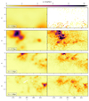 |
Fig. A.1. Extinction density a0 by Lallement et al. (2019) (left panels) and FEDReD (right panels) at several distances. The Lallement et al. (2019) data cube is interpolated in order to obtain the same resolution as this study. |
We can clearly see that density views of Lallement et al. (2019) are smoother than what we obtained with FEDReD. This is due to their hierarchical inversion with a correlation Gaussian kernel, which smoothes the structures by fitting a 3D Gaussian at each space location in a cartesian grid. For this reason, the angular resolution is smaller at short distances, while the angular resolution of FEDReD is constant and allows us to detect smaller angular structures.
All Tables
All Figures
|
Fig. 1. View of the Vela complex at 60 μm with the Improved Reprocessing of the IRAS Survey (IRIS Miville-Deschênes & Lagache 2005). The colour map is on a logarithmic scale. We overlay the approximate location of the main Vela substructures discussed in the text. |
| In the text | |
|
Fig. 2. View of the Vela complex in extinction A0 using the cumulative extinction over a distance of 5 kpc. |
| In the text | |
|
Fig. 3. Extinction density a0 at different Galactic latitudes b. x and y represent galactic coordinates, the Sun is at (0, 0) and the Galactic centre direction is to the right. We also add the contour of the clumps, their parameters being presented in Table 1. |
| In the text | |
|
Fig. 4. Extinction density a0 of the Vela complex at several distances obtained with FEDReD. The contours of each clump segmented by the FellWalker algorithm is represented with lines. |
| In the text | |
|
Fig. 5. Extinction density of the Vela complex at the distance D = 0.25 kpc and D = 0.45 kpc obtained with the Lallement et al. (2019) cube. The canonical size and location of Vela SNR and Gum Nebula (Pettersson 2008) are sketched. |
| In the text | |
|
Fig. 6. Extinction density a0 of the Vela complex at several distances obtained with FEDReD. The lines represent the contours of the cavities we extracted with the FellWalker algorithm (parameters on Table 2). |
| In the text | |
|
Fig. A.1. Extinction density a0 by Lallement et al. (2019) (left panels) and FEDReD (right panels) at several distances. The Lallement et al. (2019) data cube is interpolated in order to obtain the same resolution as this study. |
| In the text | |
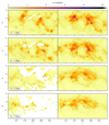 |
Fig. A.2. Continuation of Fig. A.1. |
| In the text | |
Current usage metrics show cumulative count of Article Views (full-text article views including HTML views, PDF and ePub downloads, according to the available data) and Abstracts Views on Vision4Press platform.
Data correspond to usage on the plateform after 2015. The current usage metrics is available 48-96 hours after online publication and is updated daily on week days.
Initial download of the metrics may take a while.