| Issue |
A&A
Volume 655, November 2021
|
|
|---|---|---|
| Article Number | A91 | |
| Number of page(s) | 11 | |
| Section | Stellar structure and evolution | |
| DOI | https://doi.org/10.1051/0004-6361/202038570 | |
| Published online | 25 November 2021 | |
Mass–effective temperature–surface gravity relation for intermediate-mass main-sequence stars
Ankara University, Faculty of Science, Department of Astronomy and Space Sciences, 06100 Ankara, Turkey
e-mail: This email address is being protected from spambots. You need JavaScript enabled to view it.
Received:
3
June
2020
Accepted:
30
August
2021
Abstract
Context. In this work a mass–effective temperature–surface gravity relation (MTGR) is developed for main-sequence stars in the range 6400 K ≤ Teff ≤ 20 000 K with log g ≳ 3.44. The MTGR allows the simple estimation of the masses of stars from their effective temperatures and surface gravities. It can be used for solar metallicity and can be rescaled for any metallicity within −1.0 ≤ [Fe/H] ≤ 0.7. The effect of α-enhanced compositions can also be considered with the help of correction terms.
Aims. It is aimed to develop an MTGR that can estimate the masses of main-sequence stars from their atmospheric parameters. One advantage of an MTGR over the classical mass–luminosity relations is that its mass estimation is based on parameters that can be obtained by purely spectroscopic methods, and, therefore, the interstellar extinction or reddening do not have to be known. The use of surface gravity (g) also relates an MTGR with stellar evolution and provides a more reliable mass estimation.
Methods. A synthetical MTGR is obtained from theoretical isochrones using a Levenberg-Marquardt χ2 minimization algorithm. The validity of the MTGR is then checked by testing over 278 binary components with precise absolute masses.
Results. Very good agreement has been obtained between the absolute masses of 278 binary star components and their masses estimated from the MTGR. A mathematical expression is also given to calculate the propagated uncertainties of the MTGR masses.
Conclusions. For the typical uncertainties in atmospheric parameters and metallicity (i.e., ±2.8% for Teff, ±0.1 dex for log g and ±0.15 dex for [Fe/H]) the typical uncertainties in the masses estimated from the MTGR mostly remain around 5–9%. The fact that this uncertainty level is only on average about three times as large as that of the absolute masses indicates that the MTGR is a very powerful tool for stellar mass estimation. A computer code, mtgr.pro, written in GDL or IDL is also provided for the relation.
Key words: stars: general / stars: fundamental parameters / Hertzsprung-Russell and C-M diagrams / binaries: general / stars: atmospheres
© ESO 2021
1. Introduction
Mass is generally considered to be the most important fundamental parameter of a star for many applications in astrophysics. Mass, however, can be directly derived only for multiple systems. Asteroseismology and interferometry can be used to derive the mass (and also luminosity) of single stars with little model dependence (Cunha et al. 2007; White et al. 2013). The combination of these two techniques, however, can only be applied to nearby stars of certain spectral types. Thanks to the mass–luminosity relations (MLRs), mass can be estimated for most single stars. However, the luminosity of stars cannot usually be obtained accurately from their apparent magnitude, as it requires good extinction information1 and a well-defined bolometric correction. The fact that MLRs are mostly affected by stellar evolution2 and metallicity also increases their uncertainty. Therefore, MLRs are not always the best solution for estimating the mass of single stars.
To avoid the effect of extinction, it can be useful to associate the mass with parameters purely derivable from spectroscopic methods, for example atmospheric parameters such as effective temperature (Teff) and surface gravity (g). There are many methods for deriving these parameters using the optical spectra of stars, such as the ionization or excitation equilibrium of certain elements, modeling the hydrogen Balmer lines, and measuring the Balmer jump. The atmospheric parameters derived from these methods are basically extinction-free. The use of g and [Fe/H] in these relations also allows stellar evolution and metallicity to be taken into account for the mass estimation.
The masses of single stars can be estimated from their atmospheric parameters using Teff-log g diagrams with theoretical isochrones. This method requires the retrieval and reading of the isochrones with various ages and then the interpolation of isochrone parameters for the position of the targets. Although the application of the method is not difficult, it can be time-consuming when estimating the masses of a large number of stars. Moreover, the absence of a mathematical expression of this method makes it difficult to use in computer codes. A mass–effective temperature–surface gravity relation (MTGR) may thus allow us to estimate the masses of single stars more quickly and in a more code-friendly way.
Most theoretical and observational studies attempting to understand elemental abundance distributions in the atmospheres of stars are based on their mass (see, e.g., Turcotte et al. 1998; Richer et al. 2000; Kochukhov & Bagnulo 2006; Deal et al. 2018; Monier et al. 2019). However, target stars in the observational studies may not always be members of binary systems, or, even if they are, their components may not be bright enough to be detected. In this case, an MTGR may help in estimating the stellar masses.
An MTGR not only helps in estimating the mass of single stars, but can also be used for the elemental abundance analysis of double-lined spectroscopic binaries (SB2s), particularly for long-period ones that lack accurate physical parameters. There are several groups currently working on deriving chemical abundances for binary stars (e.g., Folsom et al. 2012; Gebran et al. 2015; Torres et al. 2015). Synthetic flux spectra of the stars can be obtained via various model atmosphere codes using Teff and log g primarily. However, these theoretical spectra usually simulate the unit surface area of the stars. To obtain the composite spectrum of an SB2 system, the synthetic flux spectra of its components must be scaled by the square of the radii, and, therefore, the radius ratio of the system R1/R2 must be known. However, R1/R2 may not always be available or precise enough for long-period binaries, as long observation times are needed to cover a sufficient phase interval. Using the classical formula of gravity at a distance R from the center of a mass M, g = (GM/R2), where G is the gravitational constant, one may easily see that the following relation can be written for detached binary stars with spherical components:
If g1 and g2 can be found spectroscopically, only the mass ratio is still needed to derive the squared radius ratio. An MTGR can be used at this point as it can simply give a mass ratio from the atmospheric parameters of the components.
In this paper a mathematical MTGR model for main-sequence stars with 6400 K ≤ Teff ≤ 20 000 K and log g ≳ 3.44 is presented, which can be used in many different applications in astronomy similar to those listed above. Section 2 explains how the relation is obtained with theoretical isochrones. In Sect. 3 the validity of the MTGR is checked by testing over 278 binary components with precise absolute masses. Section 4 provides the MTGR solutions for non-solar metallicities. Section 5 gives correction terms for α-enhanced compositions. In Sect. 6 a formulation of the propagated uncertainty of mass due to the uncertainties in Teff, log g, and [Fe/H] is given. Finally, discussion and conclusion about the MTGR can be found in Sect. 7.
2. MTGR for 6400 K ≤ Teff≤ 20 000 K and log g ≳ 3.44
A large number of stars with known absolute parameters (M, Teff, and log g) are needed for a reliable MTGR as the problem is more complex than a two-parameter case, such as an MLR. The high-accuracy parameters of only several hundred detached binary components are available in the literature, and they are apparently insufficient for such a calibration. Because of this, M, Teff, and log g parameters were initially collected from the theoretical isochrones for a large Teff and log g interval to derive a “synthetic” MTGR.
The theoretical isochrones were retrieved from PARSEC (Bressan et al. 2012), mainly because it is well maintained and includes many physical processes, such as atomic diffusion and mass loss. Its web interface (CMD) is also quite versatile for the development of such a relation. The BaSTI3 (Hidalgo et al. 2018) and DARTMOUTH3 (Dotter et al. 2008) evolutionary tracks or isochrones have also been used to determine the amount of systematic errors caused by differences in the assumptions of the theoretical models. A further comparison and discussion of many other theoretical evolutionary models used nowadays can be found in Stancliffe et al. (2016).
The isochrones were retrieved for 6.60 ≤ log τ ≤ 10.13 with a step size of 0.01, where τ is the stellar age in years. The initial metallicity of the isochrones was set to Zini = 0.01774, which is the solar initial metallicity originally adopted by Bressan et al. (2012). The theoretical M, Teff, and log g trios were collected for the main-sequence phase – that is, from zero-age main sequence (ZAMS) to near4 terminal-age main sequence (TAMS) – from the isochrones. I noticed that the isochrones form a smooth surface in M-Teff-log g space between 6400 K ≤ Teff ≤ 20 000 K for main-sequence stars (red, blue, and green circles in Fig. 1) and then chose this region for an MTGR development.
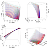 |
Fig. 1. M-Teff-log g space from various view angles for main-sequence stars with solar initial composition. The red, blue, and green circles are the points taken from PARSEC, BaSTI, and DARTMOUTH isochrones or evolutionary tracks, respectively. The cyan surface with grids is the best surface fit to the theoretical PARSEC isochrones. The surface corresponds to the synthetic MTGR formula (see text). The solid black line represents the approximate position of the ZAMS. |
Using various mathematical functions, I attempted to obtain the most appropriate expression that relates these three observational variables. To derive the coefficients of these expressions, I fit the functions to the M-Teff-log g surface using a 2D version of the Levenberg-Marquardt χ2 minimization routine (see Markwardt et al. 2009, for its 1D version). I obtained the following expression for the MTGR, which represents the theoretical M-Teff-log g surface with good accuracy, that is to say, the root-mean-square deviation (RMSD) between the PARSEC isochrones and the model is only 0.6% for M:
where5
and the coefficients are given by
The surface formed by the MTGR is shown in Fig. 1. The RMSDs of the BaSTI and DARTMOUTH tracks or isochrones from the surface are only 1.3% and 1.9% in the mass axis6. Even for the most deviating points, the deviations are always less than 5%. These deviations are in good agreement with the 1–2% mass uncertainty reported by Stancliffe et al. (2016) for 3 M⊙ tracks taken from various stellar evolution codes. These typical systematic errors of about 2% in masses can be considered as a lower uncertainty limit of the MTGR.
As we later see in Sect. 3, the above synthetic MTGR, which is derived from theoretical isochrones, agrees well with the observations. The reader may, therefore, use this MTGR to estimate the mass of main-sequence stars for 6400 K ≤ Teff ≤ 20 000 K, log g ≳ 3.44, and solar-like composition. The computer code mtgr.pro7, written in GDL8 or IDL9, can also be used for this purpose.
The MTGR can also be extrapolated for a Teff range down to 6200 K and up to 25 000 K. However, it should be noted that for these extreme values the uncertainties of the relation can be twice as large as those within the preferred Teff-log g limits. For hot stars with Teff ≥ 15 000 K, the log g limit of MTGR becomes smaller as TAMS shifts toward smaller log g values, for example 3.38 dex for 18 000 K and 3.33 dex for 20 000 K.
3. Comparison with observations
The fundamental parameters of detached binary stars have recently been compiled by Eker et al. (2018). Their catalog consists of the data of 586 components studied in the years 1975–2017 (see, e.g., Griffin & Griffin 2009; Zola et al. 2014; Bastürk et al. 2015; Özdarcan et al. 2016; Ratajczak et al. 2016; Torres et al. 2017). I used only the data in the catalog with mass measurements accurate to < 15%. I selected 278 stars in the catalog that fit the Teff, log g, and precision criteria of this study.
In Fig. 2 the absolute masses of these selected binary components have been compared to the masses derived from the MTGR with a regression line. Only 4 out of the 278 objects showed remarkable deviations (more than two times the RMSD) from the regression line. Two of these deviated objects are components of the same binary star, AG Per. The masses of its components are given as M1 = 4.498 ± 0.134 M⊙ and M2 = 4.098 ± 0.109 M⊙ in the Eker et al. (2018) catalog. However, these masses do not match the original values, M1 = 5.36 ± 0.16 M⊙ and M2 = 4.90 ± 0.13 M⊙, given by Gimenez & Clausen (1994) and might be a typo in the catalog. The same inconsistency also appears in the log g values. I consequently used the masses and surface gravities given by Gimenez & Clausen (1994) for AG Per, and the new masses indeed follow the regression line in Fig. 2 quite well. The third deviated object is the secondary component of V1388 Ori/HD 42401, whose primary component is hotter than the Teff limit of this study and was not included. The mass of the secondary component was derived as M2 = 5.16 ± 0.13 M⊙ by Williams (2009), who also reported that the star seems over-luminous for its mass on the Hertzsprung-Russell diagram (HRD). Williams (2009) noted that the He I 4471 Å line grows weaker while the Mg II 4481 Å line becomes stronger as the temperature decreases, and he used these lines to estimate the effective temperature of the star as Teff = 18 500 K. However, in his Fig. 2, the synthetic profile of He I 4471 Å is stronger and the synthetic profile of Mg II 4481 Å is weaker than those observed for the secondary component. This indicates that the effective temperature of the secondary component might be overestimated in his study. A slightly reduced effective temperature (∼16 500–17 000 K) indeed reduces the luminosity of the star and places it in a more reasonable position in the HRD (i.e., close to the evolutionary track for 5 M⊙). Using this reduced Teff, the MTGR also gives M2 ≈ 5.3 M⊙ for the star, which is very close to the absolute mass of 5.16 ± 0.13 M⊙ and makes the star very close to the regression line in Fig. 2. Nonetheless, I did not remove V1388 Ori B and used it as is for the regression analysis. The fourth and final deviated star is the primary component of GG Lup. There is no plausible reason to exclude this star in Fig. 2, and it too was retained when deriving the slope of the regression line.
 |
Fig. 2. Comparison of the absolute masses and the masses derived from the MTGR. Error bars in the y axis are the uncertainties of the absolute masses given in Eker et al. (2018). Error bars in the x axis are the propagated uncertainties for MTGR masses caused by the uncertainties in Teff and log g of the samples (see Sect. 6). For the regression line, the points are weighted according to their measurement errors. |
The slope of the final regression line in Fig. 2 is 1.001 with an almost null zero-point offset10 (−0.017). This is good observational proof showing the robustness of the synthetic MTGR. For the data and regression line, the RMSD is 0.56 M⊙ and the mean/median-absolute-deviation (MAD) is ∼0.1 M⊙. Here, the large value of RMSD arises not only from the approximations in MTGR (such as solar initial metallicity and no rotation), but also from the observational uncertainties in the Teff, log g, and MAbs. parameters of the samples. Therefore, the RMSD may not reflect the typical uncertainty of the MTGR. The MAD may also be biased and underestimated because the cataloged binary star samples are mostly concentrated in the M ≲ 2.5 M⊙ region, where the stars show less scatter in Fig. 2. By dividing the samples into two groups, I conclude that the typical uncertainties for the masses derived by the MTGR are about ±0.1 M⊙ for M ≲ 2.5 M⊙ and about ±0.3 M⊙ for M ≳ 2.5 M⊙. This roughly corresponds to a 6 − 7% typical uncertainty in mass for the cataloged binary star samples. A detailed uncertainty calculation is given in Sect. 6.
4. Effect of metallicity
One may need to constrain metallicity [M/H] or Z in the MTGR. To see how the metallicity affects the MTGR, I repeated the same procedure as in Sect. 2 for the isochrones with [M/H] = [−0.4, −0.3, −0.2, −0.1, 0.0, 0.1, 0.2, 0.3, 0.4, 0.5, 0.6, 0.7] and derived the MTGR coefficients a, b, c, d, and e for each. The corresponding Z values of these metallicities are given in the second column of Table 1. As the metallicity increases, the isochrone points shift to the lower right of the HRD, and the validity range of the MTGR, therefore, changes slightly. Table 1 gives the list of these validity ranges for various metallicities.
Validity range of the MTGR for various metallicities.
Figure 3 shows the behavior of the MTGR coefficients for various metallicities. The coefficients change slightly quadratically or cubically as a function of metallicity, except for e, which exhibits a linear tendency. These relationships can be expressed as follows:
![Mathematical equation: $$ \begin{aligned}&a = +0.037539\,\mathrm{[M/H]} ^{2}+0.106185\,\mathrm{[M/H]} +0.760313\\&b = -0.074620\,\mathrm{[M/H]} ^{3}-0.035236\,\mathrm{[M/H]} ^{2} \\&\qquad +0.139705\,\mathrm{[M/H]} +0.397282\\&c = +0.122190\,\mathrm{[M/H]} ^{3} +0.001445\,\mathrm{[M/H]} ^{2}\\&\qquad -0.387297\,\mathrm{[M/H]} +0.645036\\&d = +0.017391\,\mathrm{[M/H]} ^{3} -0.015925\,\mathrm{[M/H]} ^{2}\\&\qquad +0.021622\,\mathrm{[M/H]} -0.205739\\&e = +0.167246\,\mathrm{[M/H]} -0.191036, \end{aligned} $$](/articles/aa/full_html/2021/11/aa38570-20/aa38570-20-eq5.gif)
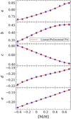 |
Fig. 3. Changes in the MTGR coefficients with metallicity. The points on the chart contain error bars. |
where11
![Mathematical equation: $$ \begin{aligned}&\mathrm {[M/H]} \simeq \mathrm{log}{\displaystyle \left( \frac{Z}{Z_{\odot }} \right)} \simeq [\mathrm{Fe/H}]. \end{aligned} $$](/articles/aa/full_html/2021/11/aa38570-20/aa38570-20-eq6.gif)
Calculating the coefficients above, the MTGR can be used for any metallicities in the range −0.4 ≲ [Fe/H]≲0.7. Masses calculated with the MTGR are greater than ∼1 M⊙ in the range where the relation is valid. Therefore, this paper mostly covers Population I stars. Although such stars are unlikely to have formed in an environment with [Fe/H] < −0.4, I also present formulae for calculating MTGR coefficients for −1.0 ≤ [Fe/H] < −0.4 in Appendix A.
I note that [Fe/H] here is the iron abundance12 of the “whole” star and does not have to be equal to the photospheric [Fe/H]. Because of atomic diffusion, the photospheric elemental abundances of stars may vary during their evolution. These variations become more evident in stars with high effective temperatures and low rotational velocities (see, e.g., Talon et al. 2006). In order to use the MTGR for stars whose photospheric chemical abundances are thought to be strongly influenced by diffusion (or by any other physical process): i) if the object is a member of a stellar group (i.e., a cluster, association or moving group), it would be best to scale the MTGR using the values of [Fe/H] or Z proposed for that group, or ii) if the object is a field star without any defined group membership, it may be more reasonable to use the original coefficients13 given in Sect. 2 instead of scaling the MTGR with the photospheric [Fe/H]. The MTGR can also be used for chemically peculiar stars, but it should never be scaled by the [Fe/H] values derived for them, as the atmospheres of these unusual objects do not represent their interiors.
5. Effect of α-enhanced composition
Current α-element abundance gradient studies for the galaxy confirm that stars can be born in environments with not only solar-like α-element abundances but also α-enhanced abundances (see, e.g., Gonzalez et al. 2011; Johnson et al. 2011; Duong et al. 2019; Hayes et al. 2020). Although the relationship between α-element and iron abundances varies from region to region (i.e., thin disk, thick disk, halo, and bulge), [α/Fe] generally tends to increase with decreasing [Fe/H] (see, e.g., Crestani et al. 2021). Since these differences in α-element abundances can affect mass calculations, this section discusses how changes in [α/Fe] can be accounted for in the MTGR.
I used the publicly available BaSTI scaled-solar and α-enhanced (Pietrinferni et al. 2021, for [α/Fe] = +0.4) stellar evolutionary tracks to characterize the effect of α-enhanced compositions on the MTGR masses. In order to avoid systematic differences between the PARSEC and BaSTI models or systematic errors due to the assumptions in the models as much as possible, I used the ratio of mass changes with α-element abundance instead of the mass values themselves. For this purpose, I define a r(Mα) ratio as follows:
![Mathematical equation: $$ \begin{aligned}&r(M_{\rm \alpha }) = \dfrac{M_{[\mathrm{\alpha /Fe}]=+0.4}}{M_{[\mathrm{\alpha /Fe}]=0.0}}-1. \end{aligned} $$](/articles/aa/full_html/2021/11/aa38570-20/aa38570-20-eq7.gif)
Here, r(Mα) represents the ratio of the masses obtained with the BaSTI models with [α/Fe]= + 0.4 and [α/Fe] = 0.0 for the same Teff, log g, and [Fe/H] values.
In order to examine the behavior of r(Mα), I retrieved BaSTI evolutionary tracks in the range 1 to 13 M⊙ in steps of 0.01 M⊙, for [Fe/H] = [−1.00, −0.75, −0.50, −0.25, 0.00] and also for [α/Fe]=[0.0, +0.4]. Figure 4 shows the calculated r(Mα) values for the evenly spaced combinations of various log Teff, log g, and [Fe/H] values (247 sets in total).
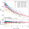 |
Fig. 4. Behavior of r(Mα) with M[α/Fe] = 0.0. Y is the mass fraction of helium used in α-enhanced models. |
It can be seen from Fig. 4 that an increase of 0.4 dex in [α/Fe] results in an increase of between 2% and 11% in mass. The magnitude of this effect decreases from low-mass stars to more massive ones. The r(Mα) values degenerate with the change in log g and [Fe/H] values. It is seen that the degeneration due to log g increases as [Fe/H] decreases. The RMSD of the scatter from the least-square logarithmic fit is 0.9%, about half the typical systematic error of 2% given in Sect. 2 for the theoretical stellar evolution models. A correction term calculated from this scatter plot, therefore, can approximately reflect the effect of α-element abundance changes on the MTGR.
By using the coefficients of the logarithmic fit, setting MMTGR ≅ M[α/Fe] = 0.0, and linearly scaling [α/Fe] abundances, the following expression was obtained:
![Mathematical equation: $$ \begin{aligned}&M_{\rm MTGR-\alpha } = M_{\rm MTGR}(1+\mathrm{[\alpha /Fe]}(k_{1}\mathrm{log}(M_{\rm MTGR})+k_{2})), \end{aligned} $$](/articles/aa/full_html/2021/11/aa38570-20/aa38570-20-eq8.gif)
where

By placing the α-element abundance ([α/Fe]) suitable for the region where the star is located and the mass of the star calculated from the MTGR (MMTGR) in the expression above, one can estimate the corrected mass (MMTGR − α) by taking into account α enhancement.
6. Estimation of mass uncertainties
The mathematical solution of the error propagation of the MTGR is quite complex because the partial derivations of the formula with respect to Teff and log g contain a large number of terms. In order to estimate the uncertainty in the mass in a more practical way, I determined the amount of change in the mass by moving Teff, log g, [M/H], and [α/Fe] in the MTGR relationship within the error limits. Assuming the uncertainties in Teff, log g, [M/H], and [α/Fe] are independent, the total uncertainty of the mass (ΔM) can be estimated from the quadrature sum formula below:
![Mathematical equation: $$ \begin{aligned}&\Delta M \simeq \sqrt{(\Delta M_{T_{\rm {eff}}})^2+(\Delta M_{\mathrm{log}\,{g}})^2+(\Delta M_{\mathrm{[M/H]}})^2+(\Delta M_{\mathrm{[\alpha /Fe]}})^2}, \end{aligned} $$](/articles/aa/full_html/2021/11/aa38570-20/aa38570-20-eq10.gif)
where ΔMTeff, ΔMlog g, ΔM[M/H], and ΔM[α/Fe] are the changes in the mass due to the uncertainty in Teff, log g, [M/H], and [α/Fe] (i.e., ΔTeff, Δlog g, Δ[M/H], and Δ[α/Fe]), respectively.
In order to obtain the expressions of ΔMTeff and ΔMlog g, I first performed a multiple linear regression analysis using the MTGR with the metallicity-independent coefficients (see Fig. B.1). From the quadrature sum of the two expressions, I obtained the following formula for estimating the mass uncertainty:
where
I then performed a similar regression analysis using the MTGR and the metallicity-dependent coefficients (see Fig. B.2) to examine the effect of metallicity on uncertainties. As can be seen from graphs 6 and 12 in Fig. B.2, the effect of [M/H] on the slopes of [ΔTeff − ΔMTeff] and [Δlog g − ΔMlog g] was negligible and was, therefore, not included in the calculations of ΔMTeff and ΔMlog g. However, parameters Teff, log g, and [M/H] all changed the slope of [Δ[M/H] − ΔM[M/H]] and were included in the calculation of ΔM[M/H] (see graphs 16–18 in Fig. B.2). From the quadrature sum of the found ΔMTeff, ΔMlog g, and ΔM[M/H] expressions, I obtained the following formula for estimating the mass uncertainty:
![Mathematical equation: $$ \begin{aligned}&\Delta M \simeq (((c_{1} T_{\rm {0}}+c_{2} {g}_0+c_{3})\Delta T_{\rm eff})^2\\&\qquad +((c_{4}T_{\rm {0}}+c_{5}{g}_{0}+c_{6})\Delta \mathrm{log}\,{g})^2 \\&\qquad +((c_{7}T_{\rm {0}}+c_{8}{g}_{0}+c_{9}\mathrm {[M/H]+c_{10}})\Delta \mathrm{{ [M/H]}})^2)^{1/2}, \end{aligned} $$](/articles/aa/full_html/2021/11/aa38570-20/aa38570-20-eq14.gif)
where
T0 and g0 are the same as in the previous expression and
![Mathematical equation: $$ \begin{aligned}&c_{1}= +2.69332\times 10^{-8}\\&c_{2}= -2.68997\times 10^{-4}\\&c_{3}= +4.67700\times 10^{-4}\\&c_{4}= +2.67543\times 10^{-4}\\&c_{5}= -3.64229\\&c_{6}= +2.58160\\&c_{7}= +7.08798\times 10^{-5}\\&c_{8}= -0.906971\\&c_{9}= -0.969023 \qquad \mathrm{(for\,the\,entire\,[M/H]\,range)}\\&c_{9}= -1.53968 \qquad \mathrm{(a\,better\,estimate\,for\,{-}0.1\,\le \,[\mathrm{M/H}]\,\le \,0.6)}\\&c_{10}= +1.07926 \qquad \mathrm{(for\,the\,entire\,[M/H]\,range)}\\&c_{10}= +1.14431 \quad \mathrm{(a\,better\,estimate\,for}\,{-}0.1\,\le \,[\mathrm{M/H}]\,\le \,0.6). \end{aligned} $$](/articles/aa/full_html/2021/11/aa38570-20/aa38570-20-eq15.gif)
Here, I presented two solutions for c9 and c10 because the behavior of [Δ[M/H] − ΔM[M/H]] slopes with [M/H] was quite nonlinear (see graph 18 in Fig. B.2).
By placing the observational variables (Teff, log g, [M/H]) and their uncertainties (ΔTeff, Δlog g, Δ[M/H]) in the expressions above, one can estimate the uncertainty in the MTGR mass (ΔM) of the star. An expanded version of the formula that includes uncertainties in α-element abundances (Δ[α/Fe]) can be found in Appendix C.
7. Discussion and conclusion
The uncertainty of the masses obtained with the MTGR depends on the uncertainties of Teff and log g by nature. The mean uncertainty of the absolute masses for the selected 278 binary components is about 2.4%, and this percentage can be regarded as the typical uncertainty for the mass derivation of binary stars in the selected Teff and log g range. This uncertainty is also on the same order as the systematic differences between different evolutionary models. When the masses of the same samples are calculated with the MTGR, the average mass uncertainty rises to only 3.8%. Considering that only the Teff and log g values of the stars are used in the MTGR, it is seen that the uncertainty level achieved is at a level that can compete with absolute mass uncertainties on average. However, one should consider here whether the atmospheric parameters obtained by spectroscopic methods are as sensitive as those obtained from simultaneous light and radial velocity curve solutions of binary stars.
It is seen that for the 278 stars in the catalog, the mean uncertainty in the Teff is 2.8%, and the mean uncertainty in log g is 0.02 dex. The typical uncertainty of 2.8% for Teff agrees well with those obtained from spectroscopic studies today (e.g., Teff = 7500 ± 200, 11 000 ± 300, 18 000 ± 500). However, the typical uncertainty of 0.02 dex for log g in binary star solutions is much more precise than the ∼0.05 − 0.20 dex uncertainties that can be achieved by spectroscopic methods (see, e.g., Kochukhov et al. 2006; Fossati et al. 2011; Gebran et al. 2016; Kılıçoğlu et al. 2018). Recent chemical abundance studies with spectral data of different quality also indicate that the iron abundance [Fe/H] of stars can be derived with an uncertainty mostly in the range 0.08–0.20 dex. If the typical uncertainties of Teff, log g, and [Fe/H] are accepted as ±2.8%, ±0.1 dex, and ±0.15 dex for spectroscopic studies, the uncertainties in the masses obtained from the MTGR are never more than 10.1% and mostly remain in the range of 5–9%. The uncertainties calculated here are propagated uncertainties due to the measurement errors of the observational variables and do not include systematic errors that may arise from phenomena such as rotation, magnetic field, surface inhomogeneity, and wind. However, the comparison between the absolute masses and calculated MTGR masses in Sect. 3 contains both random and systematic errors, and 80% of the stars appear to have a deviation of less than 10% in mass. For this reason, it is thought that systematic errors do not generally exceed random errors, with the exception of some outliers. Although these comparisons show that uncertainties in masses estimated with the MTGR are about three times higher than those in absolute masses on average, the method still has a good sensitivity in estimating the masses of single stars. The uncertainties of the spectroscopically obtained log g values should be small in order to derive more accurate masses from the MTGR.
In this study an MTGR has been developed that allows the calculation of the masses of main-sequence stars from their Teff, log g, and metallicity for 6400 K ≲ Teff ≲ 20 000 K. An expression has also been given to calculate the uncertainty of the masses derived by the relation. The mean mass uncertainty was found to be 5–9% for the typical Teff, log g, and [M/H] uncertainties that can be achieved today by analyzing stellar spectra. In order to verify and improve the accuracy of the relation, there is a great need for studies of detached binary stars with well-defined chemical abundances (particularly for [α/Fe] and [Fe/H]). Further development of the relation for a wider range of Teff and log g values may play a key role in the near future in estimating the masses of stars for spectroscopic space missions.
Spectral energy distributions (SEDs) may help in deriving the level of extinction, but for many stars it is not possible in practice to construct an SED.
For example, two stars of the same mass, one in ZAMS and the other in TAMS, may have different luminosities.
With overshooting and diffusion options.
For log g ≲ 3.55, there is a short-lived overall contraction phase in which the stars move downward in the Teff-log g diagram. This can result in two different masses from a single atmospheric parameter pair. Therefore, this contraction phase, which covers only about 1.5% of the main-sequence lifetime of stars, is not taken into account in the MTGR.
All logarithms are to the base 10.
For example, the mass estimated using the PARSEC models of a star with Teff = 10 000 K and log g = 4.0 is only 1.5% larger than that estimated with the BaSTI models.
Available from https://github.com/tolgahankilicoglu/mtgr or from the author upon request via e-mail.
GNU Data Language (Coulais et al. 2010, 2019).
Interactive Data Language.
The small offset is most likely a result of the systematic errors discussed in Sect. 2.
 does not have to be exactly equal to [Fe/H] because the metallicity Z is mostly driven by [C/H] and, particularly, [O/H]. However, [Fe/H] can be preferred to scale Z for scaled-solar compositions because iron is an element that shows a large number of lines in the spectra of the stars and its abundance is generally much more reliable than those of carbon and oxygen. A more precise approximation formula, [M/H]≃log((Z/X)/0.0207), given by Bressan et al. (2012), is used for the [M/H] values in Table 1.
![Mathematical equation: $ \mathrm{[Fe/H]}=\mathrm{log}\left( {\displaystyle \frac{N_{\mathrm{Fe, star}}}{N_{\mathrm{H, star}}}}\right)-\mathrm{log}\left({\displaystyle \frac{N_{\mathrm{Fe, \odot}}}{N_{\mathrm{H, \odot}}}}\right) $](/articles/aa/full_html/2021/11/aa38570-20/aa38570-20-eq17.gif) .
.
Corresponding to Z = 0.01774 or [M/H] ≃ 0.08653.
Acknowledgments
The author would like to thank an anonymous referee for the valuable suggestions, which significantly improved the validity range of the relation and quality of this paper. The author would also like to thank S.O. Selam, H.V. Şenavcı, Ö. Baştürk, and Ş. Çalıskan (Ankara University) for their useful comments.
References
- Bastürk, Ö., Zola, S., Liakos, A., et al. 2015, New Astron., 41, 42 [CrossRef] [Google Scholar]
- Bressan, A., Marigo, P., Girardi, L., et al. 2012, MNRAS, 427, 127 [NASA ADS] [CrossRef] [Google Scholar]
- Coulais, A. 2019, in GDL – GNU Data Language 0.9.9, eds. P. J. Teuben M. W. Pound B. A. Thomas, & E. M. Warner, ASP Conf. Ser., 523, 365 [Google Scholar]
- Coulais, A., Schellens, M., Gales, J., et al. 2010, in Status of GDL – GNU Data Language, eds. Y. Mizumoto K. I. Morita, & M. Ohishi, ASP Conf. Ser., 434, 187 [Google Scholar]
- Crestani, J., Braga, V. F., Fabrizio, M., et al. 2021, ApJ, 914, 10 [NASA ADS] [CrossRef] [Google Scholar]
- Cunha, M. S., Aerts, C., Christensen-Dalsgaard, J., et al. 2007, A&ARv, 14, 217 [NASA ADS] [CrossRef] [Google Scholar]
- Deal, M., Alecian, G., Lebreton, Y., et al. 2018, A&A, 618, A10 [NASA ADS] [CrossRef] [EDP Sciences] [Google Scholar]
- Dotter, A., Chaboyer, B., Jevremović, D., et al. 2008, ApJS, 178, 89 [Google Scholar]
- Duong, L., Asplund, M., Nataf, D. M., et al. 2019, MNRAS, 486, 3586 [NASA ADS] [CrossRef] [Google Scholar]
- Eker, Z., Bakıs, V., Bilir, S., et al. 2018, MNRAS, 479, 5491 [NASA ADS] [CrossRef] [Google Scholar]
- Folsom, C. P., Bagnulo, S., Wade, G. A., et al. 2012, MNRAS, 422, 2072 [NASA ADS] [CrossRef] [Google Scholar]
- Fossati, L., Ryabchikova, T., Shulyak, D. V., et al. 2011, MNRAS, 417, 495 [NASA ADS] [CrossRef] [Google Scholar]
- Gebran, M., Hadrava, P., Jasniewicz, G., & Richard, O. 2015, Ap&SS, 357, 137 [NASA ADS] [CrossRef] [Google Scholar]
- Gebran, M., Farah, W., Paletou, F., Monier, R., & Watson, V. 2016, A&A, 589, A83 [NASA ADS] [CrossRef] [EDP Sciences] [Google Scholar]
- Gimenez, A., & Clausen, J. V. 1994, A&A, 291, 795 [NASA ADS] [Google Scholar]
- Gonzalez, O. A., Rejkuba, M., Zoccali, M., et al. 2011, A&A, 530, A54 [NASA ADS] [CrossRef] [EDP Sciences] [Google Scholar]
- Griffin, R. E. M., & Griffin, R. F. 2009, MNRAS, 394, 1393 [NASA ADS] [CrossRef] [Google Scholar]
- Hayes, C. R., Majewski, S. R., Hasselquist, S., et al. 2020, ApJ, 889, 63 [Google Scholar]
- Hidalgo, S. L., Pietrinferni, A., Cassisi, S., et al. 2018, ApJ, 856, 125 [Google Scholar]
- Johnson, C. I., Rich, R. M., Fulbright, J. P., Valenti, E., & McWilliam, A. 2011, ApJ, 732, 108 [NASA ADS] [CrossRef] [Google Scholar]
- Kılıçoğlu, T., Çalıskan, Ş., & Ünal, K. 2018, ApJ, 852, 116 [CrossRef] [Google Scholar]
- Kochukhov, O., & Bagnulo, S. 2006, A&A, 450, 763 [NASA ADS] [CrossRef] [EDP Sciences] [Google Scholar]
- Kochukhov, O., Tsymbal, V., Ryabchikova, T., Makaganyk, V., & Bagnulo, S. 2006, A&A, 460, 831 [NASA ADS] [CrossRef] [EDP Sciences] [Google Scholar]
- Markwardt, C. B. 2009, in Astronomical Data Analysis Software and Systems XVIII, eds. D. A. Bohlender D. Durand, & P. Dowler, ASP Conf. Ser., 411, 251 [NASA ADS] [Google Scholar]
- Monier, R., Griffin, E., Gebran, M., et al. 2019, AJ, 158, 157 [NASA ADS] [CrossRef] [Google Scholar]
- Özdarcan, O., Çakırlı, Ö., & Akan, C. 2016, New Astron., 46, 47 [CrossRef] [Google Scholar]
- Pietrinferni, A., Hidalgo, S., Cassisi, S., et al. 2021, ApJ, 908, 102 [NASA ADS] [CrossRef] [Google Scholar]
- Ratajczak, M., Hełminiak, K. G., Konacki, M., et al. 2016, MNRAS, 461, 2234 [NASA ADS] [CrossRef] [Google Scholar]
- Richer, J., Michaud, G., & Turcotte, S. 2000, ApJ, 529, 338 [Google Scholar]
- Stancliffe, R. J., Fossati, L., Passy, J.-C., & Schneider, F. R. N. 2016, A&A, 586, A119 [NASA ADS] [CrossRef] [EDP Sciences] [Google Scholar]
- Talon, S., Richard, O., & Michaud, G. 2006, ApJ, 645, 634 [Google Scholar]
- Torres, G., Sandberg Lacy, C. H., Pavlovski, K., Fekel, F. C., & Muterspaugh, M. W. 2015, AJ, 150, 154 [Google Scholar]
- Torres, G., McGruder, C. D., Siverd, R. J., et al. 2017, ApJ, 836, 177 [Google Scholar]
- Turcotte, S., Richer, J., & Michaud, G. 1998, ApJ, 504, 559 [Google Scholar]
- White, T. R., Huber, D., Maestro, V., et al. 2013, MNRAS, 433, 1262 [Google Scholar]
- Williams, S. J. 2009, AJ, 137, 3222 [NASA ADS] [CrossRef] [Google Scholar]
- Zola, S., Şenavcı, H. V., Liakos, A., Nelson, R. H., & Zakrzewski, B. 2014, MNRAS, 437, 3718 [NASA ADS] [CrossRef] [Google Scholar]
Appendix A: MTGR coefficients for stars with −1.0 ≤ [M/H] < −0.4
Validity range of the MTGR for −1.0 ≤ [M/H] < −0.4.
a = −0.213170 [M/H] + 0.641994 (for −0.5 ≤ [Fe/H] < −0.4)
a = +0.080416 [M/H] + 0.788564 (for −1.0 ≤ [Fe/H] < −0.5)
b = +0.051362 [M/H]2 + 0.175915 [M/H] + 0.402455
c = +0.500361 [M/H]3 + 1.059979 [M/H]2 + 0.447992 [M/H] + 0.831917
d = −0.040907 [M/H]2 + 0.024522 [M/H] − 0.201473
e = +0.215200 [M/H] − 0.174482
 |
Fig. A.1. Changes in the MTGR coefficients with metallicity in the range −1.0 ≤ [M/H] ≤ −0.4. |
Appendix B: Regression analysis for the uncertainty expressions
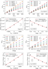 |
Fig. B.1. Regression analysis and determining the coefficients in the uncertainty estimation formula for the MTGR with the metallicity-independent coefficients. The zero points (ZPs) c3 and c6 were calculated by averaging the individual calculations, i.e., c3 = (c3[1]+c3[2])/2 and c6 = (c6[1]+c6[2])/2. |
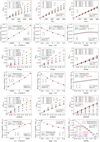 |
Fig. B.2. Regression analysis and calculating the coefficients in the uncertainty estimation formula for the MTGR with the metallicity-dependent coefficients. The slopes in graphs 6 and 12 were too small and ignored (see text). Two solutions were provided for c9 and c10: Regression line 1 is for the entire [M/H] range, and regression line 2 is a better estimate for −0.1 ≤ [M/H] ≤ 0.6. The zero points (ZPs) c3, c6, and c10 were calculated by averaging the individual calculations, i.e., c3 = (c3[1]+c3[2])/2, c6 = (c6[1]+c6[2])/2, and c10 = (c10[1]+c10[2]+c10[3])/3. |
Appendix C: Uncertainty estimation formula, including uncertainties in [α/Fe]
![Mathematical equation: $$ \begin{aligned}\Delta M \simeq &(((c_{1} T_{\rm{0}}+c_{2} g_0+c_{3})\Delta T_{\rm eff})^2 + \\&\qquad ((c_{4}T_{\rm{0}}+c_{5}g_{0}+c_{6})\Delta{\rm log}\,g)^2 + \\&\qquad ((c_{7}T_{\rm{0}}+c_{8}g_{0}+c_{9}\rm{[M/H]+c_{10}})\Delta{\rm { [M/H]}})^2 + \\&\qquad (((c_{11}{\rm log}(M_{\rm MTGR})+c_{12})M_{\rm MTGR}\Delta[{\rm \alpha/Fe}])^2)^{1/2}, \end{aligned} $$](/articles/aa/full_html/2021/11/aa38570-20/aa38570-20-eq18.gif)
where
T0 = Teff − 13 200 K
g0 = log g − 3.8
Δ[α/Fe]= uncertainty of [α/Fe]
MMTGR is the mass calculated by the MTGR
c1 = +2.69332 ⋅ 10−8
c2 = −2.68997 ⋅ 10−4
c3 = +4.67700 ⋅ 10−4
c4 = +2.67543 ⋅ 10−4
c5 = −3.64229
c6 = +2.58160
c7 = +7.08798 ⋅ 10−5
c8 = −0.906971
c9 = −0.969023 (for the entire [M/H] range)
c9 = −1.53968 (a better estimate for −0.1 ≤ [M/H] ≤ 0.6)
c10 = +1.07926 (for the entire [M/H] range)
c10 = +1.14431 (a better estimate for −0.1 ≤ [M/H] ≤ 0.6)
c11 = k1 = −0.17
c12 = k2 = 0.255.
All Tables
All Figures
|
Fig. 1. M-Teff-log g space from various view angles for main-sequence stars with solar initial composition. The red, blue, and green circles are the points taken from PARSEC, BaSTI, and DARTMOUTH isochrones or evolutionary tracks, respectively. The cyan surface with grids is the best surface fit to the theoretical PARSEC isochrones. The surface corresponds to the synthetic MTGR formula (see text). The solid black line represents the approximate position of the ZAMS. |
| In the text | |
|
Fig. 2. Comparison of the absolute masses and the masses derived from the MTGR. Error bars in the y axis are the uncertainties of the absolute masses given in Eker et al. (2018). Error bars in the x axis are the propagated uncertainties for MTGR masses caused by the uncertainties in Teff and log g of the samples (see Sect. 6). For the regression line, the points are weighted according to their measurement errors. |
| In the text | |
|
Fig. 3. Changes in the MTGR coefficients with metallicity. The points on the chart contain error bars. |
| In the text | |
|
Fig. 4. Behavior of r(Mα) with M[α/Fe] = 0.0. Y is the mass fraction of helium used in α-enhanced models. |
| In the text | |
|
Fig. A.1. Changes in the MTGR coefficients with metallicity in the range −1.0 ≤ [M/H] ≤ −0.4. |
| In the text | |
|
Fig. B.1. Regression analysis and determining the coefficients in the uncertainty estimation formula for the MTGR with the metallicity-independent coefficients. The zero points (ZPs) c3 and c6 were calculated by averaging the individual calculations, i.e., c3 = (c3[1]+c3[2])/2 and c6 = (c6[1]+c6[2])/2. |
| In the text | |
|
Fig. B.2. Regression analysis and calculating the coefficients in the uncertainty estimation formula for the MTGR with the metallicity-dependent coefficients. The slopes in graphs 6 and 12 were too small and ignored (see text). Two solutions were provided for c9 and c10: Regression line 1 is for the entire [M/H] range, and regression line 2 is a better estimate for −0.1 ≤ [M/H] ≤ 0.6. The zero points (ZPs) c3, c6, and c10 were calculated by averaging the individual calculations, i.e., c3 = (c3[1]+c3[2])/2, c6 = (c6[1]+c6[2])/2, and c10 = (c10[1]+c10[2]+c10[3])/3. |
| In the text | |
Current usage metrics show cumulative count of Article Views (full-text article views including HTML views, PDF and ePub downloads, according to the available data) and Abstracts Views on Vision4Press platform.
Data correspond to usage on the plateform after 2015. The current usage metrics is available 48-96 hours after online publication and is updated daily on week days.
Initial download of the metrics may take a while.