| Issue |
A&A
Volume 654, October 2021
|
|
|---|---|---|
| Article Number | A145 | |
| Number of page(s) | 12 | |
| Section | The Sun and the Heliosphere | |
| DOI | https://doi.org/10.1051/0004-6361/202141524 | |
| Published online | 22 October 2021 | |
Large-amplitude longitudinal oscillations in solar prominences simulated with different resolutions
1
Instituto de Astrofísica de Canarias, 38205 La Laguna, Tenerife, Spain
e-mail: This email address is being protected from spambots. You need JavaScript enabled to view it.
2
Departamento de Astrofísica, Universidad de La Laguna, 38206 La Laguna, Tenerife, Spain
3
Departament de Física, Universitat de les Illes Balears, 07122 Palma de Mallorca, Spain
4
Institute of Applied Computing and Community Code (IAC3), UIB, La Palma, Spain
Received:
11
June
2021
Accepted:
28
July
2021
Abstract
Context. Large-amplitude longitudinal oscillations (LALOs) in solar prominences have been widely studied in recent decades. However, their damping and amplification mechanisms are not well understood.
Aims. In this study, we investigate the attenuation and amplification of LALOs using high-resolution numerical simulations with progressively increasing spatial resolutions.
Methods. We performed time-dependent numerical simulations of LALOs using the 2D magnetic configuration that contains a dipped region. After the prominence mass loading in the magnetic dips, we triggered LALOs by perturbing the prominence mass along the magnetic field. We performed the experiments with four values of spatial resolution.
Results. In the simulations with the highest resolution, the period shows good agreement with the pendulum model. The convergence experiment revealed that the damping time saturates at the bottom prominence region with increasing resolution, indicating the existence of a physical reason for the damping of oscillations. At the prominence top, the oscillations are amplified during the first minutes and are then slowly attenuated. The characteristic time suggests more significant amplification in the experiments with the highest spatial resolution. The analysis revealed that the energy exchange between the bottom and top prominence regions is responsible for the attenuation and amplification of LALOs.
Conclusions. High-resolution experiments are crucial when studying the periods and the damping mechanism of LALOs. The period agrees with the pendulum model only when using a sufficiently high spatial resolution. The results suggest that numerical diffusion in simulations with insufficient spatial resolution can hide important physical mechanisms, such as amplification of oscillations.
Key words: Sun: corona / Sun: filaments / prominences / Sun: oscillations / methods: numerical
© ESO 2021
1. Introduction
Solar prominences are clouds of cold and dense plasma suspended in the solar corona, supported against gravity by the magnetic field. They are subject to various types of oscillations. These periodic motions are classified as small-amplitude and large-amplitude oscillations according to their velocity (see reviews by Oliver & Ballester 2002; Arregui et al. 2018). In the large-amplitude oscillations (LAOs), a large portion of the prominence oscillates with amplitudes that exceed 10 km s−1. If the plasma motions are directed along the magnetic field, the oscillations are classified as large-amplitude longitudinal oscillations (LALOs). On the contrary, oscillations with velocity directed perpendicular to the magnetic field are called transverse LAOs. More information on the classification and properties of the different types of oscillations can be found in the last update of the living review by Arregui et al. (2018).
Jing et al. (2003, 2006) were first to report the LALOs in solar prominences. Since then, many observations have provided important information on the properties of LALOs (see, e.g., Vršnak et al. 2007; Zhang et al. 2012, 2017; Li & Zhang 2012; Luna et al. 2014; Bi et al. 2014). Observations have shown that the period of the LALOs is around 1 hour, and the damping time is usually less than two periods, indicating strong attenuation of the motions. Luna et al. (2018) cataloged the filament oscillations using several months of the Global Oscillation Network Group (GONG) Hα data near the maximum of solar cycle 24. The catalog provides a large sample of the LALOs and statistics of the periods and damping times. On average, these latter authors found that the ratio of damping time to period is equal to 1.25, in agreement with the earlier observations. An intriguing phenomenon in the prominence oscillations is the amplification of motions. Contrary to the damping caused by energy loss, oscillations somehow acquire additional energy and increase their amplitudes in time. The first amplification event was reported by Molowny-Horas et al. (1999) from time-series of Hβ filtergrams of a polar crown prominence. These authors measured a periodic Doppler signal and found clear oscillations with periods of between 60 and 95 min and damping times between 119 and 377 min at six locations of the prominence. At one of the locations, they also found an oscillation with a period of 28 min and a growing amplitude with a characteristic time of 140 min. More recently, Zhang et al. (2017) reported the observation of LALOs in which the oscillatory amplitude remains constant or increases with time in some regions of the prominence. This unusual behavior of the LALO amplitude has also been found in the GONG catalog by Luna et al. (2018; see, e.g., Fig. 25).
In recent decades, LALOs have been studied in many analytical and numerical works. These were dedicated to answering questions related to the restoring and damping mechanisms. Luna & Karpen (2012) proposed a so-called pendulum model where the main contribution to the restoring force is the gravity projected along the magnetic field. This model suggests that the period is defined by the radius of curvature of the magnetic field (see also Roberts 2019, for another description of the model). The following studies, based on the analytical calculations or the 2D and 3D simulations, confirmed that the pendulum model describes the periods of longitudinal oscillations quite well under typical prominence conditions (e.g., Luna et al. 2012, 2016; Zhou et al. 2018; Zhang et al. 2019; Liakh et al. 2020; Fan 2020). Zhou et al. (2018) found a systematic discrepancy of some 10% with respect to the pendulum model. These latter authors suggested that the longitudinal oscillations produce dynamical deformations of the field structure. Under these circumstances, the period of LALOs can be slightly longer than predicted by the pendulum model due to the flattening of the magnetic field by the plasma motions. Zhang et al. (2019) found that in the regime of a relatively weak magnetic field, when the gravity-to-Lorentz-force ratio is close to unity, the trajectory of the prominence plasma is not along the rigid field lines. The authors found that these dynamic deformations of the magnetic structure contribute to the damping of the oscillations. Similarly, Fan (2020) found discrepancies with respect to the pendulum model also associated with the dynamical deformation of the field lines during the oscillations.
Many candidate damping mechanisms have been proposed to explain the observed LALO attenuation. Radiative losses and thermal conduction were considered by Zhang et al. (2012) and Zhang et al. (2019) as damping mechanisms for LALOs. These authors pointed out the importance of taking nonadiabatic effects into consideration; however, using numerical simulations, they showed that nonadiabatic effects alone are not sufficient to explain the observed damping (see also Zhang et al. 2020). Zhang et al. (2013) and Ruderman & Luna (2016) proposed an alternative mechanism for the attenuation of LALOs. Zhang et al. (2013) considered the possibility of LALOs decaying due to the mass drainage, while Ruderman & Luna (2016) studied the damping due to mass accretion. Both studies showed that either the mass drainage or mass accretion results in a decreasing velocity of the prominence. As a consequence, this leads to the damping of oscillations. Zhang et al. (2019) found that in a situation of a relatively weak magnetic field, the wave leakage is an important mechanism for LALO damping, in addition to the nonadiabatic effects. The motion of the prominence mass produces perturbations in the field structure that emanate in the form of magnetohydrodynamic (MHD) waves.
In order to explain both the damping and the amplification of prominence oscillations, Ballester et al. (2016) derived an expression for the temporal variation of the background temperature, taking into account the radiative losses and thermal conduction. The authors concluded that using some combination of the characteristic times of the different mechanisms and increasing or decreasing the background temperature could lead to damping or amplification of the oscillations. Zhang et al. (2017) proposed an alternative mechanism to explain the amplification: the threads located at the different dips of the same flux tube interchange their energy. Using 1D numerical simulations, Zhou et al. (2017) studied the different combinations of the active–passive threads and demonstrated that the energy exchange significantly affects the damping or amplification time of the LALOs. However, this mechanism cannot explain the amplification of the threads that belong to the different field lines.
All the studies of LALOs in 2D and 3D have been done using numerical simulations. In these numerical experiments, dissipation is unavoidable. Terradas et al. (2016) investigated the influence of the numerical dissipation on the prominence oscillations in the 3D model, increasing spatial resolution up to 300 km. These latter authors concluded that the energy losses associated with the numerical dissipation are significantly reduced in the high-resolution experiments. In more recent 3D simulations, Adrover-González & Terradas (2020) and Fan (2020) pointed out that the reduction in numerical dissipation is crucial when studying the damping of LALOs. Terradas et al. (2013), Luna et al. (2016), and Zhang et al. (2019) performed 2D numerical experiments of the prominence oscillation with spatial resolution up to 125 and 156 km, respectively. These numerical simulations showed significant damping which might be partly contributed by numerical diffusivity. Liakh et al. (2020) studied the convergence of a 2.5D experiment of LALOs excited in a magnetic flux rope. The authors performed an experiment with a spatial resolution of 60 km and compared it to a similar experiment with a spatial resolution of 240 km. They found that the periods of LALOs are consistent in the two experiments, although the damping time becomes longer in the higher resolution experiment. They therefore concluded that in their experiments, the attenuation of LALOs is associated mainly with numerical dissipation.
In this work, we aim to understand the physical origin of the LALO damping and the other processes usually hidden by the artificial dissipation in numerical experiments. To this end, we performed 2D convergence experiments with progressively increasing spatial resolutions up to the highest value of 30 km.
This paper is organized as follows: In Sect. 2 the numerical model is described. In Sects. 3 and 4 we explain the temporal evolution of the plasma under the disturbance directed along the field and compare the oscillatory parameters in the experiments with the different spatial resolution and the different prominence layers. In Sect. 5 we summarize the main results.
2. Initial configuration
We assume a 2D prominence model as shown in Fig. 1. The model is defined in the Cartesian coordinate system in the xz-plane, where z-axis corresponds to the vertical direction. The initial magnetic field is a potential configuration which contains a dipped part suitable to support a prominence. The magnetic configuration is composed of periodic arcades defined as
 (1)
(1)
 (2)
(2)
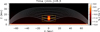 |
Fig. 1. Density distribution and magnetic field lines at the central part of the computational domain after the mass loading and relaxation processes. The dashed lines denote the initial magnetic field prior to the mass loading. |
where B0 = 33 G, x0 = 0 Mm, and z0 = −2 Mm. We also set  and k2 = 3k1 where D = 191.4 Mm, that is the half-size of the numerical domain along the x-direction. The superposition of the major and minor arcades form the magnetic field structure shown in Fig. 1 with the dipped part centered at x = 0 Mm and between z = 0 and 25 Mm. As shown in the figure, the curvature of the magnetic field lines decreases with height. For z > 27 Mm, the magnetic field lines change from concave-up to concave-down, becoming ordinary loops. A detailed description of this magnetic configuration is given by Terradas et al. (2013) and Luna et al. (2016). The magnetic field strength varies between 9.0 and 12.5 G from the bottom to the top of the dipped region (z = 8 − 25 Mm). The magnetic field strength lies in the range of the values obtained from the magnetic field measurements in the solar prominences (Leroy et al. 1983, 1984).
We assume an initial atmosphere consisting of a stratified plasma in hydrostatic equilibrium, including the chromosphere, transition region (TR), and corona. The temperature profile is given by
![Mathematical equation: $$ \begin{aligned} T(z)= T_{0} + \frac{1}{2} \left(T_{c}-T_{0} \right) \left[1+ \tanh \left( \frac{z-z_{c}}{W_z}\right) \right] . \end{aligned} $$](/articles/aa/full_html/2021/10/aa41524-21/aa41524-21-eq4.gif) (3)
(3)
We choose Tc = 106 K, T0 = 104 K, Wz = 0.4 Mm, and zc = 3.6 Mm. In this profile the temperature ranges from Tch = 104 K at the base of the chromosphere to Tc = 106 K in the corona. As the plasma is stratified in the vertical direction, the density changes from ρ = 9 × 10⁻⁹ kg m−3 in the chromosphere to ρ = 1.69 × 10⁻¹² kg m−3 at the base of the corona at the height zc = 3.6 Mm.
We numerically solve ideal MHD equations using the MANCHA3D code (Khomenko et al. 2008; Felipe et al. 2010; Khomenko & Collados 2012). The governing equations of mass, momentum, internal energy, induction equation, and the corresponding source terms are described in Felipe et al. (2010). The computation domain consists of a box of 384 × 108 Mm in size. In order to study the influence of the numerical diffusivity on the prominence oscillations, we use four spatial resolutions with Δ = 240, 120, 60 and 30 km from the coarse to the fine grids. We assume a periodic condition at the left and right boundaries. At the bottom boundary, we apply the current-free condition for the magnetic field (see, e.g., Luna et al. 2016) and a symmetric condition for the temperature and pressure. At the bottom boundary, the density is fixed. At the top boundary, the zero-gradient condition is applied to all the variables except for Bx. We impose that Bx is antisymmetric.
In order to add the prominence mass to the dipped region of the magnetic field, we use artificial mass loading, as described by Liakh et al. (2020). We use the source term in the continuity equation to increase the density in the dipped region of the magnetic field. The density source term distribution is a Gaussian function (see Eq. (9) from Liakh et al. 2020 work) centered at (x, z) = (0, 11.8) Mm. The mass loading starts at t = 0 s and ends at t = 100 s. The resulting prominence has a density of 110 times the density of the initial corona with dimensions of 5 and 9 Mm in the horizontal and vertical directions, respectively.
During the first 8.3 min, we use intensive artificial damping in order to minimize the undesirable motions caused by the response of the magnetic field to the mass-loading process. Figure 1 shows the prominence after this relaxation phase. The dashed lines denote the initial magnetic field. As we can see, the magnetic field lines are slightly elongated downwards due to the heavy prominence mass. The prominence itself also has some deformation, becoming more compressed toward the center of the dip, and slightly drops down with respect to the initial height. At the end of the relaxation process, the system is close to static equilibrium.
Similarly to our previous work (Liakh et al. 2020), we trigger oscillation after the relaxation phase by applying an external force over the prominence. This force is incorporated as a source term in the momentum equations as
 (4)
(4)
 (5)
(5)
where tpert = 10 s is the duration of the disturbance that starts at t = 8.3 min. The parameters σx = σz = 12 Mm are the half-sizes of the perturbed region in the horizontal and vertical directions centered at (xpert, zpert) = (0, 12) Mm. The force given by Eqs. (4) and (5) is directed along the local magnetic field in contrast to our previous work (Liakh et al. 2020) where the perturbation is purely horizontal or vertical. The maximum velocity of the perturbation is vpert = 22 km s−1, which is in the range of the observed amplitudes of LAOs (see review by Arregui et al. 2018). In order to study the long-term evolution of prominence motions, we run the experiments for 275 min of physical time.
3. Influence of spatial resolution on prominence dynamics
In this work, we study the influence of the numerical diffusivity in the LAOs by progressively increasing the spatial resolution as described in Sect. 1. Figure 2 shows an example of the temporal evolution after the perturbation for Δ = 30 km. This kind of evolution is representative of all our numerical experiments. After the initial disturbance at t = 8.3 min, the prominence moves to the right along the magnetic field and reaches its maximum initial displacement at approximately t = 17 min (Fig. 2a). We see that the maximum horizontal displacement is large at the upper prominence part, whereas the bottom part is only slightly displaced from the equilibrium position. The reason is that, as the initial perturbation launches the prominence mass along the field lines with similar velocities, the plasma reaches different horizontal locations as the field lines have different curvatures. Figure 2b shows the prominence at t = 45.3 min. At this time, the prominence has reached its maximum displacement on the left side and begins to move again toward the right. The top part of the prominence slightly delays from the rest of the prominence body, suggesting a longer oscillation period. Figures 2c and d show the prominence evolution after several cycles of oscillations. From the velocity field displayed by the purple arrows, we can see that the prominence layers oscillate out of phase producing counterstreaming flows. Such counterstreaming flows are commonly observed in the filaments (Schmieder et al. 1991; Zirker et al. 1998; Lin et al. 2005). Chen et al. (2014) claimed that these counterstreaming motions are associated with oscillations. The oscillation period depends on the physical conditions of the magnetic field line where the prominence plasma resides. This means that the period can vary slightly for the neighboring field lines. This explains a phase difference between the motions of the prominence layers, shown in Fig. 2c. In addition, these alternate motions can be associated with processes of evaporation and condensation in prominences (Zhou et al. 2020) or shock downstreams produced by jets (Luna & Moreno-Insertis 2021).
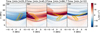 |
Fig. 2. Temporal evolution of v∥, magnetic field, and the prominence mass after the perturbation. Dashed black lines denote unperturbed magnetic field lines; solid black lines are the actual magnetic field lines at a given moment; orange lines are density isocontours, and purple arrows are the velocity field. Spatial resolution: Δ = 30 km. |
In order to study the prominence plasma oscillations, we analyze the bulk motions of the plasma in the two possible polarizations: transverse and longitudinal to the magnetic field. Following our previous works (Luna et al. 2016; Liakh et al. 2020) we compute the velocities of the center of mass of independent field lines using Eqs. (5) and (6) from Luna et al. (2016). The parameters v∥ and v⊥ are the longitudinal and transverse velocities of the center of mass of each field line. First, we select 20 equally spaced field lines that permeate the prominence body at the height from 7.2 Mm up to 17.6 Mm. We then start integrating the field lines in the chromosphere, where the magnetic field remains unchanged according to the line-tying condition. As our fluid is perfectly conducting, the frozen-in condition is fulfilled. This allows us to advect the motions in the same field line at any moment in time. We selected an identical set of field lines for each numerical experiment in order to compare the resulting velocities.
Figure 3 shows the temporal evolution of v∥ for the four numerical experiments with different spatial resolutions. The global behavior of the prominence is similar in each of the experiments. After the initial perturbation at t = 8.3 min, the longitudinal velocity increases in all the lines. The longitudinal velocity reaches the highest value, v∥ = 22 km s−1, in the densest prominence part at a height of z = 11.8 Mm. At t = 15 − 35 min, we see a certain shift in the signal. This phase shift is related to the different periods associated with the different field lines. On the one hand, we see that the oscillations are less attenuated with increasing spatial resolution, although the difference between the cases Δ = 60 and 30 km is less pronounced. On the other hand, the behavior of the damping changes with height. This is in agreement with the visual impression from Fig. 2, discussed above. Oscillations at the bottom and in the central part are strongly damped in all the experiments. At the height of 13 − 17 Mm, the oscillations with weaker attenuation last for a longer time. In the highest-resolution simulation, the upper prominence part keeps oscillating with a significant amplitude even at the final stage of the numerical experiment.
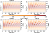 |
Fig. 3. Temporal evolution of v∥ at the center of mass at the selected field lines. The color bar denotes the maximum initial density at each field line. The left vertical axis indicates the velocity amplitude scale. The right vertical axis denotes the vertical location of the dips of selected magnetic field lines. |
3.1. Influence of spatial resolution on the period
Figure 4 shows the periods of the longitudinal oscillations for each of the 20 selected field lines and each numerical experiment with different spatial resolutions. The period is more or less uniform under 10.2 Mm and above 16.1 Mm. In contrast, for heights z = 10.2 − 16.1 Mm, we see an increase in period with the height of the magnetic dip. These heights correspond to the prominence region with the highest density contrast. One can observe in this figure that the slope of the curves depends on the spatial resolution. The steepest slope corresponds to the experiment with the highest spatial resolution (Δ = 30 km). In contrast, for Δ = 240 km, the period is more uniform with a smoother variation with height.
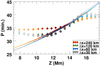 |
Fig. 4. Periods as a function of height of the magnetic dips. The symbols denote the longitudinal period obtained from the numerical experiments, and the solid lines are the periods predicted by the pendulum model. Different colors and symbols correspond to the experiments with different spatial resolutions. The color gradation from dark to light corresponds to a decrease in the density contrast. |
Under prominence conditions, the main restoring force of these oscillations is the solar gravity projected along the magnetic field (see e.g., Luna & Karpen 2012; Luna et al. 2012, 2016; Zhou et al. 2018; Liakh et al. 2020; Fan 2020). Luna & Karpen (2012) suggested that the period of the longitudinal oscillations depends only on the radius of curvature of the magnetic dip, Rc, as
 (6)
(6)
where g = 274 m s−2 is the solar gravitational acceleration. In our magnetic configuration, the curvature of the magnetic field lines in the prominence area decreases with height. This implies that the period of the different field lines increases with height in agreement with Fig. 3. The radius of curvature of the dips of the field lines changes with time in response to plasma motion. In order to compare the results of the simulations with the pendulum model, we compute the time-averaged radius of curvature. The values obtained are Rc = 17.3 − 51.1 Mm for the selected field lines from the bottom to the top of the dipped region. With Eq. (6) we computed the theoretical period shown in Fig. 4 as a solid line. From the figure, we see that for the experiments with Δ = 30, 60, and 120 km, we see good agreement between the numerical results and the pendulum model at heights z = 10.2 − 16.1 Mm, where the body of the prominence is located. We also observe that even though all three resolutions show good agreement with the pendulum model, the agreement is slightly better for the finest resolution. In contrast, in the coarse case with Δ = 240 km, there is only agreement at the central part of the prominence. This indicates a strong influence of the numerical diffusivity on the period of oscillations and shows that a certain spatial resolution is necessary to reach agreement with the pendulum model. Using 3D numerical simulations, Zhou et al. (2018) and Fan (2020) concluded that in their experiments the disagreement with the pendulum model is of the order of 10 %. We suggest that high-resolution experiments can reduce this discrepancy.
Figure 4 shows a clear deviation from the pendulum model below the prominence, z < 10.2 Mm, and above it, z > 16 Mm, even for high spatial resolution. This behavior suggests the existence of a physical reason for the deviation. Previous works (such as Zhou et al. 2018; Zhang et al. 2019; Liakh et al. 2020; Fan 2020) have also found discrepancies with the pendulum model. Zhou et al. (2018) and Zhang et al. (2019) found that if the gravity-to-Lorentz-force ratio is close to unity, the heavy prominence plasma can significantly deform the magnetic field lines. They defined the dimensionless parameter as the ratio between the weight of the thread and the magnetic pressure, as
 (7)
(7)
where l is the half-length of the prominence thread. The authors argued that if the parameter δ is close to unity, the weight of the prominence changes the field geometry dynamically. In this situation, the actual trajectory of the plasma does not coincide with the field lines, and the trajectory of the plasma has a larger radius of curvature than the one corresponding to an unperturbed magnetic field line (see Fig. 9 from Zhang et al. 2019). Thus, the resulting period of LALOs can be longer than predicted by the pendulum model. In our model, the magnetic field at the dipped part increases with z, from 9 G at the base of the prominence up to 12 G at its top. Using the parameters of our model, we obtain that the maximum value δ = 0.7 reached at around z = 11.8 Mm, which is around the densest region of the prominence. In that region, we obtain good agreement with the pendulum model. For the regions below and above the prominence, δ is much smaller. We conclude that the weakness of the magnetic field cannot explain the discrepancies between the pendulum model and our simulations. However, we find that the interaction between the longitudinal motion of the prominence and the magnetic structure is not negligible. When the prominence moves, the magnetic field structure changes considerably. These perturbations of the magnetic field could be transmitted to the rest of the field structure. This contributes to the damping of the LALOs due to wave leakage, as we discuss below in Sect. 4.
Luna et al. (2012) showed that the restoring force of LALOs is a combination of the gravity projected along the magnetic field and the gas pressure gradient. The relative importance of both restoring forces depends on the radius of curvature of the field lines with respect to a characteristic radius Rlim. In a situation where Rc ≪ Rlim, the gravity dominates, and the pendulum model is valid. In contrast, for Rc ≳ Rlim the gas pressure term dominates. The radius Rlim depends on several parameters of the structure
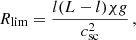 (8)
(8)
where csc is coronal sound speed, L is half-length of the field line, and χ is the density contrast between the prominence and the ambient corona. In our situation, below the prominence (z < 10.2 Mm), the ratio Rc/Rlim > 0.2, and it increases for smaller values of z. The main reason is that the density contrast χ is close to 1 in that region. This indicates that the contribution of the gas pressure to the restoring force is important, and the pendulum model is no longer valid. Similarly, for z ≥ 16.1 Mm, both the curvature of the field lines and the density contrast decrease with height. Thus Rc/Rlim increases in these field lines from 0.4 up to 5.9 for higher values of z. This explains why the period of the longitudinal oscillations deviates from the pendulum period for locations below and above the prominence. In turn, in the central region, z = 10.2 − 16.1 Mm, the ratio is around 0.1.
The prominence is also subject to transverse oscillations. Similarly to the longitudinal velocity, we obtained the temporal evolution of v⊥ using Eq. (6) from Luna et al. (2016) for each selected field line. Figure 5 shows the temporal evolution for the Δ = 30 km case. We only show the case with the finest spatial resolution because all experiments have a very similar temporal evolution of the transverse velocity. From the figure, we see that the transverse motions are synchronized in all the field lines with the same oscillatory period, P = 4 min. This uniformity of the oscillations shows that the motion is related to a global normal mode of the field structure. The oscillation in v⊥ is not harmonic, and the amplitude is modulated every approximately 30 min. This modulation is also synchronized in all the field lines shown in the figure. The amplitude of the transverse oscillations is equal to 5 km s−1, which is much smaller than for the longitudinal motions. This modulation of the amplitude is probably related to the motion of the prominence mass. The global motion of the plasma periodically changes the characteristics of the magnetic structure, resulting in a modulation of the oscillation. The signal modulation of the transverse velocity can also indicate the longitudinal to transverse mode conversion. This could be the subject of future work. During the simulation time, the transverse oscillations show nearly no significant damping in the four numerical experiments with different Δ, indicating that numerical dissipation does not affect this kind of motion.
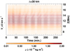 |
Fig. 5. Temporal evolution of v⊥ at the center of mass of the selected field lines. The color bar denotes the maximum initial density at each field line. The left vertical axis indicates the velocity amplitude scale. The right axis denotes the height of the dips of the field lines. |
3.2. Influence of spatial resolution on the damping
In order to study in detail the damping in the experiments with different Δ, we consider longitudinal velocity in two field lines with dips at z = 11.8 Mm (central part of the prominence) and z = 16.1 Mm (top part). The v∥ in the central and top field lines are shown in Fig. 6. The upper panel of Fig. 6 shows that the attenuation is strongest in the experiment with the coarsest resolution (Δ = 240 km). The oscillation signal is almost completely damped after 150 min. In contrast, the experiment with Δ = 30 km is where we observe the weakest attenuation. Comparing all the cases, we see that the damping time increases for increasing spatial resolution (i.e., decreasing Δ). The curves for Δ = 60 and 30 km are relatively close to each other. This indicates that the damping time is close to the saturation and that the high-resolution experiment shows indications of physical damping not associated with numerical diffusivity. In order to quantify the damping time, we fit the signal of v∥ with a decaying sinusoidal function such as v∥ = V0e−t/τdsin(2πt/P + ϕ). The values of τd obtained from the best fit to v∥ are shown in Fig. 7 (top panel) as a function of spatial resolution, Δ. We observe that the damping time increases when Δ decreases for experiments with Δ = 240, 120, and 60 km. In these three experiments, the damping time shows a quadratic dependence on Δ denoted by the solid line in the top panel of Fig. 7. The trend marked by the solid line seems to indicate the damping time of about τd = 110 min as Δ approaches zero. However, the damping time in the experiment with Δ = 30 km deviates from this quadratic trend and has a similar value to the one in the Δ = 60 km experiment. We fitted an arctangent function to all four values of τd, including the one in Δ = 30 km experiment. This new fit is shown as a dashed line at the top panel of Fig. 7. The trend, including the highest resolution case, deviates from the quadratic trend as the curve becomes flatter. This suggests that τd may saturate for decreasing values of Δ showing the non-numerical (i.e., physical) origin of this damping. According to the dashed line, τd → 100 min as Δ approaches zero.
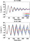 |
Fig. 6. Temporal evolution of v∥ at the center of mass of the selected field lines. Top: field line close to the prominence center. Bottom: field line at the top part of the prominence. The different colors distinguish the experiments with different spatial resolutions. |
We repeated the same analysis for the magnetic field line located at z = 16.1 Mm, which is at the top of the prominence. The results are shown in the bottom panel of Fig. 6. The temporal evolution of the longitudinal velocity differs significantly from the one at z = 11.8 Mm. We can clearly distinguish two stages in temporal evolution. In the first stage, the velocity is amplified after the initial perturbation. The amplification is more significant and extended in time in the simulations with higher spatial resolution. For the case of Δ = 30 km, the amplitude increases from v∥ = 19.5 km s−1 up to 23 km s−1 over 130 min. This amplification can be clearly traced in the snapshots of temporal evolution shown in Fig. 2d above. The oscillations are attenuated in the bottom and central parts of the prominence. However, at heights z > 15 Mm, the displacement is not only comparable to but is even larger than the initial displacement shown in Fig. 2a.
During the second stage, the oscillations begin to decay slowly. At the end of the simulated time (t = 275 min), the motions are almost completely damped for the experiments with Δ = 240, 120 km. In the higher resolution simulations, Δ = 30 and 60 km, the upper prominence part oscillates undamped for a longer time. In order to quantify the damping time for these complex oscillations, we split the velocity signal into two parts associated with the amplification and damping. We then fit v∥ with the decaying and amplifying sinusoidal functions. For the amplification stage, we assume the characteristic time, τA, to be negative, and for the decaying stage, we assume the damping time, τD, to be positive. From the best fit to the longitudinal velocity, we obtain values of τA in the range [−600,−225] min, and values of τD in the range of [152,628] min. The higher values of both parameters correspond to better resolutions. The results of this analysis are shown in the bottom panel of Fig. 7. The characteristic time of the amplification, τA, differs significantly between the high- and low-resolution experiments. We observe that, in the experiment with Δ = 30 km, τA = −225 min, which is the most significant amplification. In addition, the bottom panel of Fig. 6 shows that this amplification stage is more extended in time for the finer spatial resolutions. The damping time in the second phase reaches a value of τD = 628 min for the simulation with Δ = 30 km, indicating the weakest damping. The amplification stage is not as relevant for the experiment with Δ = 240 km. For this experiment, the amplification time τA = −600 min is the longest, and the oscillations have an almost constant amplitude during the first 67.8 min. We performed a fit to both τA and τD using an arctangent function, allowing us to find the trend for both parameters (Fig. 7, solid lines at the bottom panel). With these trends, we can roughly estimate that the real physical amplification for our system would have a characteristic time of −200 min, whereas the damping time would be longer than 900 min. These results may indicate that our highest-resolution experiment is about to resolve a physical mechanism for these effects.
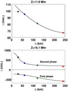 |
Fig. 7. Top: damping time of oscillations at a height of 11.8 Mm as a function of the spatial resolution Δ. The solid line denotes the quadratic dependence, and the dashed line shows fitting with an arctangent function. Bottom: same for the height 16.1 Mm. The solid lines denote fitting with an arctangent function. |
4. Physical reasons for the amplification and damping of oscillations
As we have shown in Sect. 3.2 above, oscillations at the bottom part of the prominence damp quickly, and those at the top part are initially amplified and damped later. We have also seen that these phenomena may have a physical origin and are not related to numerical dissipation. In this section, we perform a detailed analysis to shed light on the possible physical mechanisms that produce these effects.
First, we study the contributions of the different forces to the energy balance in two regions of the prominence defined by the orange rectangles in Fig. 1.
Equations (9)–(11) show the temporal derivatives of the work done by the different forces in the region, which we denote Σ. In addition, Eq. (12) gives the kinetic energy flow along the boundaries of the region, ∂Σ. These equations are:
 (9)
(9)
 (10)
(10)
 (11)
(11)
 (12)
(12)
where n is the vector normal to the region boundaries. The combination of the four terms is equal to the temporal derivative of the kinetic energy integrated in the region Σ,  . Figure 8 shows the temporal evolution of the terms given by Eqs. (9–12). All these magnitudes are shown with respect to their values at t = 8.5 min. The top and bottom panels of the figure show the quantities computed in the top and bottom regions shown in Fig. 1, respectively.
 |
Fig. 8. Work done by the gravity force (brown line), by the gas pressure force (light green line), by the Lorentz force (light blue line), and the kinetic energy flow (pink line) integrated in two rectangles shown by the orange lines in Fig. 1. The black lines denote a total kinetic energy variation with respect to its value at t = 8.5 min. |
Figure 8 shows a clear difference in the evolution of the plasma in both regions of the prominence. At the top of the structure, the kinetic energy decreases rapidly immediately after the initial perturbation. The curve oscillates around an average value that seems to increase slightly from approximately 30 to 100 min. The amplification of the oscillations at the upper part of the prominence does not result in a significant increase in the kinetic energy because the region of integration is larger than the prominence size and includes the nonamplified regions. After t = 100 min, the kinetic energy decreases. Figure 8 (top panel) shows that the gas pressure work is negative and that it makes the largest contribution to the kinetic energy losses after t = 100 min. In contrast, the work done by the Lorentz force in the first 100 min is positive, indicating that it accelerates the prominence plasma. In turn, the kinetic energy inflow through the boundaries is relatively small compared to the other terms.
At the bottom part of the prominence (Fig. 8, bottom panel), the black line shows a substantial decrease in the first 100 min coinciding with the significant attenuation of the oscillations in this region. The bottom panel shows that the main contribution to the kinetic energy losses is associated with the work of the gas pressure and the Lorentz force. This may indicate the generation of fast MHD waves, which are emitted from the prominence region. This mechanism can contribute to the damping of the oscillations, as already suggested by Zhang et al. (2019). These fast waves are associated with the gas pressure and the Lorentz forces. Additional evidence for the wave leakage is shown in Fig. 9, which shows the time–distance diagram of the transverse velocity, v⊥, along the axis, x = 0 Mm, over 10 min. The fast MHD waves produce perturbations of the v⊥ field. The figure shows the waves that travel upwards with a pattern of alternating positive and negative values of v⊥. The inclination of the ridges is indicative of the speed of the waves. As we performed the experiments in the low-β regime, the speed of the fast waves is approximately the Alfvén speed, vA. The dashed lines represent locations of a wave front that would propagate at a local Alfvén speed. We can see that the waves emitted from the prominence propagate with speed similar to the Alfvén speed. Figures 8 and 9 indicate that an important portion of the energy of the prominence oscillation is emitted in the form of fast MHD waves.
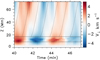 |
Fig. 9. Time–distance diagram of the transverse velocity, v⊥, along the vertical direction at the horizontal position x = 0 Mm. Black horizontal lines denote the position of the prominence. Dashed lines denote the position of a hypothetical wave front propagating at a local Alfvén speed. |
Figure 8 demonstrates that the increase in WB at the top may be related to its decrease at the bottom part of the structure. Therefore, not all the energy losses at the bottom of the prominence are emitted in the form of waves. Instead, a part of this energy is transferred to the top of the structure. This transfer can explain the amplification of the oscillations at the upper part of the prominence.
We computed the incoming Poynting flux into two regions shown by the orange lines in Fig. 1 as
 (13)
(13)
Figure 10 shows the time integral of the incoming Poynting flux in both regions. We can see that during the time interval 65 − 150 min, the incoming Poynting flux at the prominence top dominates over the outcoming flux. This indicates that the magnetic energy increases at the upper prominence region. The opposite situation occurs at the bottom region. The magnetic energy leaves the region, and the time integral of the Poynting flux has a negative sign. In addition, the shapes of both curves are similar but are of opposite phase with respect to each other, indicating that the top part gains a significant part of the energy lost by the bottom part. Apart from this energy transfer, the flux at the bottom part also shows the leakage of energy emitted to the ambient atmosphere in the form of fast waves. Overall, Fig. 10 indicates that magnetic energy seems to be partially transferred from the bottom to the top of the prominence.
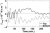 |
Fig. 10. Time-integrated magnetic energy inflow through the boundaries of the domains indicated by orange lines in Fig. 1. The short-period component has been filtered out. |
In order to understand the physical reason for the transfer of the energy from the bottom to the upper layers of the prominence, we computed the time–distance diagrams of the different contributions to the total energy along the vertical direction integrated in the region from x = −12 Mm to x = 12 Mm. The result of this calculation is shown in Fig. 11. The three panels show the kinetic energy density, ek = ρv2/2 (Fig. 11a), the magnetic energy density, eB = B2/2μ0 (Fig. 11b), and the gravitational energy density, eg = ρgz (Fig. 11c), at times immediately after the perturbation. We are interested in the variation of these energies after the mass loading. Therefore, Fig. 11 shows the difference with respect to the values of each of the energies at t = 8.3 min. The light and dark fringes reflect the plasma motions and velocity variations. The figure clearly shows the phase shift between the oscillations at different heights inside the prominence. In addition, it can be observed that the kinetic energy increases at t = 60 − 130 min and at heights z > 13 Mm. A similar increase can be seen for the magnetic and gravitational energies in Figs. 11b and c. The magnetic energy increase is associated with the energy exchange between the bottom and top parts of the prominence, as was already shown in Fig. 10. The gravitational energy increases during the same period of time which is related to the amplification of the oscillation velocities at the top of the prominence. As plasma is accelerated, it can reach greater heights along the magnetic field. As a result, the total gravitational energy increases. At the bottom, in the region of strong attenuation, we can see the energy losses in all the panels. As mentioned before, some fraction of the energy is taken away by the fast MHD waves, and some other fraction is transferred to upper prominence layers.
 |
Fig. 11. Time–distance diagram of the energy variations with respect to their values immediately before the perturbation, e − e0, integrated in the region from x = −12 Mm to x = 12 Mm. The white lines denote the heights where the prominence is located. (a) Kinetic energy density, ek = ρv2/2; (b) magnetic energy density, eB = B2/2μ0; (c) gravitational energy density, eg = ρgz. |
The results above seem to indicate that the amplification of the oscillations is related to the energy transfer from the bottom to the top parts of the structure. The magnetic field structure changes with time thanks to the oscillations, and the actual trajectory of the plasma motions is no longer along the unperturbed magnetic field lines. In a situation with a rigid magnetic field, the trajectory coincides with the field line, and the Lorentz force has no projection along the trajectory of the plasma. However, in our situation, the trajectory does not coincide with the unperturbed field lines. In such a case, the forces along the trajectory can become different from the forces projected along the magnetic field lines. In order to understand the detailed mechanism for the amplification and damping, we study the motion of the individual fluid elements by integrating the velocity field at each moment in time. We selected two plasma elements with the initial coordinates (x, z) = (0, 16.1) and (0, 11.8) Mm which correspond to the particles at the top and the central part of the prominence.
In order to highlight the modifications of the magnetic field lines due to the plasma motions, we multiply the magnetic field perturbation by a factor of ten. This magnetic field is defined as B′ = 10(B − B0)+B0, where B is the actual magnetic field at time t and B0 is the magnetic field at t = 0 min. Similarly, the displacement of the fluid elements is also multiplied by the same factor in order to fulfill the frozen-in condition. Figure 12 shows the positions of the fluid elements (orange diamonds) and centers of the dips (blue circles) of the magnetic field lines at the different moments in time. Figure 12a shows the maximum displacement of the fluid elements immediately after the perturbation. We see that the field lines hosting the particles change, and the positions of the dips follow the motion of the particles. In Fig. 12b, the fluid elements move to the left of the structure. The dip at the lower line continues following the particle motion. In contrast, at the upper line, the dip is located ahead of the particle. In this situation, the upper particle reaches the dip in a position that is displaced to the left of the original dip. Thus, the upper particle has gained an increment in velocity during this first half period of oscillation. This process is repeated during the following period. In Fig. 12c, we observe that the particle has gained energy and that the amplitude of the oscillation is larger. In Fig. 12d, the dip has moved away from the particle again, leading to an increase in the amplitude. The same process is also produced in the reverse direction, as can be observed in Figs. 12e and f. The motion of the upper dip follows the motion of the dip at the bottom line. The reason for this is that the magnetic structure reacts to the bulk motion of the prominence. In this sense, the changes in the magnetic configuration at the bottom part of the structure affect the top part of the structure.
 |
Fig. 12. Temporal evolution of the fluid elements and the magnetic field lines after the perturbation. The orange diamonds denote the positions of the fluid elements, and the blue circles correspond to the locations of the center of each dip. The purple arrows denote the velocity field. Dotted lines are unperturbed magnetic field lines; solid lines are actual magnetic field lines at a given moment. We note that the magnetic field perturbation is multiplied by a factor of ten for better visibility. |
The situation is exactly the opposite at the bottom of the structure. The plasma motions also modify the field lines, but the dip approaches the particle in this case. In this way, the oscillatory amplitude is reduced in each oscillation period. In Figs. 12c and d, we observe the following situation: the motion of the fluid element at the bottom causes displacement of the corresponding magnetic dip. As we can see from Figs. 12e and f, the dip at the bottom continues following the fluid element in the next period of oscillations. Thus, the particle continues losing energy in each period, and the oscillations damp quickly.
In order to study the oscillation amplification phenomena in more detail and check how the motions at the upper and lower part of the prominence affect each other, we performed an alternative experiment described below. We used the same prominence model, but the height of the maximum of the perturbation was shifted down to z = 9 Mm, and the characteristic vertical size of the perturbed region was reduced to σz = 4.8 Mm. Using this numerical setup, we excited the prominence oscillations only at the bottom, while the upper part of the prominence remained unperturbed. We then repeated the calculations of v∥, as was done in Sect. 3. Figure 13 shows v∥ at the selected field lines. We observe that the motions of the plasma at heights of 7.2 − 10.2 Mm are produced directly by the perturbation. These oscillations are significantly attenuated during the time interval shown in Fig. 13. No perturbation has been applied for the field lines with z > 10.2 Mm, and therefore v∥ at those field lines is initially zero. However, after 20 min of evolution, we observe a signature of oscillations with a small amplitude at the upper part. After 20 min, the oscillation fronts reach the top of the prominence, and their amplitude increases. At the time 100 − 150 min, we can clearly see oscillation at z > 10.2 Mm. We also observe the phase shift of the signal between different heights, which resembles Fig. 3. We additionally performed the opposite experiment perturbing the top region and leaving the bottom and central part without initial perturbation. The analysis of motions revealed a similar result, namely that the oscillations at the top drive the oscillations at the bottom layers of the prominence. This experiment seems to indicate that the transfer of energy could be symmetric. However, in the regular experiments where all the layers are excited simultaneously, the bottom part of the prominence drives the motion producing the amplification of the top part. The coupling of the oscillations of the different regions of prominence is a very interesting subject for future research.
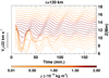 |
Fig. 13. Temporal evolution of v∥ at the center of mass of the selected field lines in the experiment with the perturbation at the bottom. The color bar denotes the maximum initial density at each field line. The left vertical axis indicates the velocity amplitude scale. The right vertical axis denotes the height of the dips of the field lines. |
In order to check if oscillation amplification is a common phenomenon of LALOs, we performed yet another experiment. Here, we did not use any external perturbation but instead loaded the prominence mass at some distance from the center of the magnetic dips. As the mass is not in equilibrium, it starts to move under the action of gravity in the direction toward the center of the dips. Thus, the plasma starts to oscillate around the equilibrium position, and the LALOs are established without any disturbance. We find that the resulting oscillations in this experiment are similar to those obtained in the previous experiments. Namely, we observe that the velocity at the top of the prominence increases while at the bottom of the prominence, it rapidly decreases. After several cycles of oscillations, the velocity of the plasma at the upper prominence region becomes high enough to allow plasma to leave the shallow dips. Consequently, the acceleration of the plasma at the top leads to mass drainage from the upper prominence region.
Summarizing all of above, we conclude that the effect of amplification of the plasma at the prominence top takes place in several alternative experiments, such as experiments where we perturb only the bottom part of the prominence or do not apply perturbation but place prominence in a nonequilibrium position. This means that the effect of amplification is a frequent ingredient of LALOs and deserves further investigation in the future.
5. Summary and conclusions
We studied the properties of LALOs, including their periods and damping mechanism, based on 2D numerical simulations. We used a simple magnetic field configuration that includes a dipped region. After the mass loading in the dips, we applied a perturbation to the prominence. This perturbation was directed along the magnetic field. Our main goal was to investigate the physical mechanism of attenuation of the LALOs covered by the numerical diffusion. Therefore, we studied the oscillations in the same numerical model while gradually increasing spatial resolution, Δ.
We analyzed the prominence motions and computed the periods in the different prominence regions. The period of the oscillations shows an increase with height. We also find that the period depends on Δ. In the higher resolution simulations, the period shows a strong dependence on height, while in the lower resolution experiments, this dependence is less pronounced. The period shows good agreement with the pendulum model in our simulations with the highest resolution, namely of 30 km.
We studied the damping of oscillations in different experiments and at different prominence regions. In all the experiments, the bottom part of the prominence is characterized by strong attenuation of oscillations. This attenuation is present even in the highest resolution experiments. The experiments with the finest resolution, Δ = 60 and 30 km, demonstrated that further improvement of the spatial resolution does not significantly affect the damping time. This means that our experiments reached the resolution where the damping of oscillations is no longer associated with the numerical dissipation but is rather caused by some physical mechanism. In a real situation, additional effects such as thermal conduction and radiative losses also contribute to the damping. It is necessary to include these additional effects in order to understand which mechanism dominates in damping of the LALOs. This will be the subject of future research.
Our experiments revealed that oscillations at the prominence top are amplified during the first 130 min of simulations and are later slowly attenuated. The amplification appears to be more efficient and extended in time in the high-resolution experiments.
In order to explain the strong attenuation of oscillations at the prominence bottom and their simultaneous amplification at the prominence top, we analyzed the evolution of different types of energies in the corresponding regions. This analysis revealed that the damping of the oscillations is partially due to the collective work done by the gas pressure and Lorentz force. The energy is emitted in the form of fast magneto-acoustic waves. This result is in agreement with the findings of Zhang et al. (2019). Furthermore, we see that the damping of the oscillations is related to the strength of the magnetic field. The motion of the prominence plasma produces periodic changes in the magnetic field. We find that this effect leads to the generation of fast MHD waves. The time–distance diagram of the transverse velocity provides another piece of evidence for the wave leakage. The inclination of the wave front ridges found in the time–distance diagram is in agreement with the inclination predicted by the Alfvén speed. Yet another conclusion from our analysis is that the Lorentz force plays an important role in the damping and amplification of LALOs. While at the bottom, it contributes to the kinetic energy losses and acts to decelerate plasma, at the top of the prominence the work done by the Lorentz force is positive and provides the gain in energy needed for amplification of oscillations. The analysis of the Poynting flux revealed that a significant portion of the energy leaving the bottom part is transferred to the top. These results suggest that the energy losses in the lower region of the prominence are caused by both wave leakage and energy and momentum transfer to the upper prominence region.
Our study of LALOs based on 2D numerical simulations shows that high spatial resolution is crucial for investigating the periods of LALOs. The period agrees with the pendulum model only when the spatial resolution is sufficiently high. High spatial resolution is also important for understanding the damping of LALOs. On the other hand, the numerical dissipation can hide important physical mechanisms such as amplification of LALOs.
In the future, it will be useful to study the attenuation and amplification mechanisms further using high-resolution experiments with more complex 3D setups, which would allow us to take the mechanism of resonant absorption into consideration. Furthermore, it is also desirable to include nonadiabatic effects. This could allow us to study the relative importance of the mechanisms described in this paper with respect to the resonant absorption and nonadiabatic effects. On the other hand, more observations are needed to further study the phenomena of the amplified prominence oscillations.
Acknowledgments
V. Liakh acknowledges the support of the Instituto de Astrofísica de Canarias via an Astrophysicist Resident fellowship. M. Luna acknowledges support through the Ramón y Cajal fellowship RYC2018-026129-I from the Spanish Ministry of Science and Innovation, the Spanish National Research Agency (Agencia Estatal de Investigación), the European Social Fund through Operational Program FSE 2014 of Employment, Education and Training and the Universitat de les Illes Balears. V.L. and M.L. also acknowledge support from the International Space Sciences Institute (ISSI) via team 413 on “Large-Amplitude Oscillations as a Probe of Quiescent and Erupting Solar Prominences”. E.K. thanks the support by the European Research Council through the Consolidator Grant ERC-2017-CoG-771310-PI2FA and by the Spanish Ministry of Economy, Industry and Competitiveness through the grant PGC2018-095832-B-I00 is acknowledged. V. Liakh, M. Luna, and E. Khomenko thankfully acknowledge the technical expertise and assistance provided by the Spanish Supercomputing Network (Red Española de Supercomputacíon), as well as the computer resources used: the LaPalma Supercomputer, located at the Instituto de Astrofísica de Canarias. The authors thankfully acknowledge the computer resources at MareNostrum4 and the technical support provided by Barcelona Supercomputing Center (RES-AECT-2020-1-0012 and RES-AECT-2020-2-0010)
References
- Adrover-González, A., & Terradas, J. 2020, A&A, 633, A113 [NASA ADS] [CrossRef] [EDP Sciences] [Google Scholar]
- Arregui, I. N., Oliver, R., & Ballester, J. L. 2018, Liv. Rev. Sol. Phys., 15, 3 [NASA ADS] [CrossRef] [Google Scholar]
- Ballester, J. L., Carbonell, M., Soler, R., & Terradas, J. 2016, A&A, 591, A109 [NASA ADS] [CrossRef] [EDP Sciences] [Google Scholar]
- Bi, Y., Jiang, Y., Yang, J., et al. 2014, ApJ, 790, 100 [NASA ADS] [CrossRef] [Google Scholar]
- Chen, P. F., Harra, L. K., & Fang, C. 2014, ApJ, 784, 50 [NASA ADS] [CrossRef] [Google Scholar]
- Fan, Y. 2020, ApJ, 898, 34 [Google Scholar]
- Felipe, T., Khomenko, E., & Collados, M. 2010, ApJ, 719, 357 [Google Scholar]
- Jing, J., Lee, J., Spirock, T. J., et al. 2003, ApJ, 584, L103 [NASA ADS] [CrossRef] [Google Scholar]
- Jing, J., Lee, J., Spirock, T. J., & Wang, H. 2006, Sol. Phys., 236, 97 [NASA ADS] [CrossRef] [Google Scholar]
- Khomenko, E., & Collados, M. 2012, ApJ, 747, 87 [Google Scholar]
- Khomenko, E., Collados, M., & Felipe, T. 2008, Sol. Phys., 251, 589 [NASA ADS] [CrossRef] [Google Scholar]
- Leroy, J. L., Bommier, V., & Sahal-Brechot, S. 1983, Sol. Phys., 83, 135 [NASA ADS] [CrossRef] [Google Scholar]
- Leroy, J. L., Bommier, V., & Sahal-Brechot, S. 1984, A&A, 131, 33 [Google Scholar]
- Li, T., & Zhang, J. 2012, ApJ, 760, L10 [NASA ADS] [CrossRef] [Google Scholar]
- Liakh, V., Luna, M., & Khomenko, E. 2020, A&A, 637, A75 [NASA ADS] [CrossRef] [EDP Sciences] [Google Scholar]
- Lin, Y., Engvold, O., Rouppe van der Voort, L., Wiik, J. E., & Berger, T. E. 2005, Sol. Phys., 226, 239 [Google Scholar]
- Luna, M., & Karpen, J. 2012, ApJ, 750, L1 [NASA ADS] [CrossRef] [Google Scholar]
- Luna, M., & Moreno-Insertis, F. 2021, ApJ, 912, 75 [NASA ADS] [CrossRef] [Google Scholar]
- Luna, M., Díaz, A. J., & Karpen, J. 2012, ApJ, 757, 98 [Google Scholar]
- Luna, M., Knizhnik, K., Muglach, K., et al. 2014, ApJ, 785, 79 [NASA ADS] [CrossRef] [Google Scholar]
- Luna, M., Terradas, J., Khomenko, E., Collados, M., & de Vicente, A. 2016, ApJ, 817, 157 [Google Scholar]
- Luna, M., Karpen, J., Ballester, J. L., et al. 2018, ApJS, 236, 35 [NASA ADS] [CrossRef] [Google Scholar]
- Molowny-Horas, R., Wiehr, E., Balthasar, H., Oliver, R., & Ballester, J. L. 1999, JOSO Annu. Rep., 1998, 126 [NASA ADS] [Google Scholar]
- Oliver, R., & Ballester, J. L. 2002, Sol. Phys., 206, 45 [NASA ADS] [CrossRef] [Google Scholar]
- Roberts, B. 2019, MHD Waves in the Solar Atmosphere (Cambridge: Cambridge University Press) [Google Scholar]
- Ruderman, M. S., & Luna, M. 2016, A&A, 591, A131 [NASA ADS] [CrossRef] [EDP Sciences] [Google Scholar]
- Schmieder, B., Raadu, M. A., & Wiik, J. E. 1991, A&A, 252, 353 [NASA ADS] [Google Scholar]
- Terradas, J., Soler, R., Díaz, A. J., Oliver, R., & Ballester, J. L. 2013, ApJ, 778, 49 [Google Scholar]
- Terradas, J., Soler, R., Luna, M., et al. 2016, ApJ, 820, 125 [Google Scholar]
- Vršnak, B., Veronig, A. M., Thalmann, J. K., & Žic, T. 2007, A&A, 471, 295 [NASA ADS] [CrossRef] [EDP Sciences] [Google Scholar]
- Zhang, Q. M., Chen, P. F., Xia, C., & Keppens, R. 2012, A&A, 542, A52 [NASA ADS] [CrossRef] [EDP Sciences] [Google Scholar]
- Zhang, Q. M., Chen, P. F., Xia, C., Keppens, R., & Ji, H. S. 2013, A&A, 554, A124 [NASA ADS] [CrossRef] [EDP Sciences] [Google Scholar]
- Zhang, Q. M., Li, T., Zheng, R. S., Su, Y. N., & Ji, H. S. 2017, ApJ, 842, 27 [CrossRef] [Google Scholar]
- Zhang, L. Y., Fang, C., & Chen, P. F. 2019, ApJ, 884, 74 [Google Scholar]
- Zhang, Q. M., Guo, J. H., Tam, K. V., & Xu, A. A. 2020, A&A, 635, A132 [NASA ADS] [CrossRef] [EDP Sciences] [Google Scholar]
- Zhou, Y.-H., Zhang, L.-Y., Ouyang, Y., Chen, P. F., & Fang, C. 2017, ApJ, 839, 9 [NASA ADS] [CrossRef] [Google Scholar]
- Zhou, Y.-H., Xia, C., Keppens, R., Fang, C., & Chen, P. F. 2018, ApJ, 856, 179 [Google Scholar]
- Zhou, Y. H., Chen, P. F., Hong, J., & Fang, C. 2020, Nat. Astron., 4, 994 [NASA ADS] [CrossRef] [Google Scholar]
- Zirker, J. B., Engvold, O., & Martin, S. F. 1998, Nature, 396, 440 [Google Scholar]
All Figures
|
Fig. 1. Density distribution and magnetic field lines at the central part of the computational domain after the mass loading and relaxation processes. The dashed lines denote the initial magnetic field prior to the mass loading. |
| In the text | |
|
Fig. 2. Temporal evolution of v∥, magnetic field, and the prominence mass after the perturbation. Dashed black lines denote unperturbed magnetic field lines; solid black lines are the actual magnetic field lines at a given moment; orange lines are density isocontours, and purple arrows are the velocity field. Spatial resolution: Δ = 30 km. |
| In the text | |
|
Fig. 3. Temporal evolution of v∥ at the center of mass at the selected field lines. The color bar denotes the maximum initial density at each field line. The left vertical axis indicates the velocity amplitude scale. The right vertical axis denotes the vertical location of the dips of selected magnetic field lines. |
| In the text | |
|
Fig. 4. Periods as a function of height of the magnetic dips. The symbols denote the longitudinal period obtained from the numerical experiments, and the solid lines are the periods predicted by the pendulum model. Different colors and symbols correspond to the experiments with different spatial resolutions. The color gradation from dark to light corresponds to a decrease in the density contrast. |
| In the text | |
|
Fig. 5. Temporal evolution of v⊥ at the center of mass of the selected field lines. The color bar denotes the maximum initial density at each field line. The left vertical axis indicates the velocity amplitude scale. The right axis denotes the height of the dips of the field lines. |
| In the text | |
|
Fig. 6. Temporal evolution of v∥ at the center of mass of the selected field lines. Top: field line close to the prominence center. Bottom: field line at the top part of the prominence. The different colors distinguish the experiments with different spatial resolutions. |
| In the text | |
|
Fig. 7. Top: damping time of oscillations at a height of 11.8 Mm as a function of the spatial resolution Δ. The solid line denotes the quadratic dependence, and the dashed line shows fitting with an arctangent function. Bottom: same for the height 16.1 Mm. The solid lines denote fitting with an arctangent function. |
| In the text | |
|
Fig. 8. Work done by the gravity force (brown line), by the gas pressure force (light green line), by the Lorentz force (light blue line), and the kinetic energy flow (pink line) integrated in two rectangles shown by the orange lines in Fig. 1. The black lines denote a total kinetic energy variation with respect to its value at t = 8.5 min. |
| In the text | |
|
Fig. 9. Time–distance diagram of the transverse velocity, v⊥, along the vertical direction at the horizontal position x = 0 Mm. Black horizontal lines denote the position of the prominence. Dashed lines denote the position of a hypothetical wave front propagating at a local Alfvén speed. |
| In the text | |
|
Fig. 10. Time-integrated magnetic energy inflow through the boundaries of the domains indicated by orange lines in Fig. 1. The short-period component has been filtered out. |
| In the text | |
|
Fig. 11. Time–distance diagram of the energy variations with respect to their values immediately before the perturbation, e − e0, integrated in the region from x = −12 Mm to x = 12 Mm. The white lines denote the heights where the prominence is located. (a) Kinetic energy density, ek = ρv2/2; (b) magnetic energy density, eB = B2/2μ0; (c) gravitational energy density, eg = ρgz. |
| In the text | |
|
Fig. 12. Temporal evolution of the fluid elements and the magnetic field lines after the perturbation. The orange diamonds denote the positions of the fluid elements, and the blue circles correspond to the locations of the center of each dip. The purple arrows denote the velocity field. Dotted lines are unperturbed magnetic field lines; solid lines are actual magnetic field lines at a given moment. We note that the magnetic field perturbation is multiplied by a factor of ten for better visibility. |
| In the text | |
|
Fig. 13. Temporal evolution of v∥ at the center of mass of the selected field lines in the experiment with the perturbation at the bottom. The color bar denotes the maximum initial density at each field line. The left vertical axis indicates the velocity amplitude scale. The right vertical axis denotes the height of the dips of the field lines. |
| In the text | |
Current usage metrics show cumulative count of Article Views (full-text article views including HTML views, PDF and ePub downloads, according to the available data) and Abstracts Views on Vision4Press platform.
Data correspond to usage on the plateform after 2015. The current usage metrics is available 48-96 hours after online publication and is updated daily on week days.
Initial download of the metrics may take a while.