| Issue |
A&A
Volume 653, September 2021
|
|
|---|---|---|
| Article Number | A61 | |
| Number of page(s) | 14 | |
| Section | Stellar structure and evolution | |
| DOI | https://doi.org/10.1051/0004-6361/202141100 | |
| Published online | 08 September 2021 | |
Probing galactic double-mode RR Lyrae stars against Gaia EDR3
Konkoly Observatory, Research Center for Astronomy and Earth Sciences, Eötvös Loránd Research Network, 1121 Konkoly Thege ut. 15-17, Budapest, Hungary
e-mail: This email address is being protected from spambots. You need JavaScript enabled to view it.
Received:
15
April
2021
Accepted:
7
June
2021
Abstract
Context. Classical double-mode pulsators (RR Lyrae stars and δ Cepheids) are important because of their simultaneous pulsation in low-order radial modes. This enables us to place stringent constraints on their physical parameters.
Aims. We use 30 bright galactic double-mode RR Lyrae (RRd) stars to estimate their luminosities and compare these luminosities with those derived from the parallaxes of the recent data release (EDR3) of the Gaia survey.
Methods. We employed pulsation and evolutionary models together with observationally determined effective temperatures to derive the basic stellar parameters.
Results. When we exclude six outlying stars (e.g., those with blending issues), the RRd and Gaia luminosities correlate well. With the adopted temperature zeropoint from one of the works based on the infrared flux method, we find it necessary to increase the Gaia parallaxes by 0.02 mas to bring the RRd and Gaia luminosities into agreement. This value is consonant with those derived from studies on binary stars in the context of Gaia. We also examined the resulting period-luminosity-metallicity (PLZ) relation in the 2MASS K band as follows from the RRd parameters. This leads to the verification of two independently derived other PLZs. No significant zeropoint differences are found. Furthermore, the predicted K absolute magnitudes agree within σ = 0.005 − 0.01 mag.
Key words: stars: fundamental parameters / stars: variables: RR Lyrae / stars: oscillations / stars: horizontal-branch / stars: distances
© ESO 2021
1. Introduction
The historical discovery of the first double-mode RR Lyrae star, AQ Leo, in the galactic field by Jerzykiewicz & Wenzel (1977) and the subsequent discovery of ten additional objects by Cox et al. (1983) in the globular cluster M15 opened the possibility of deriving masses of RR Lyrae stars directly from linear pulsation models, independently of stellar evolution theory. This is an important step in understanding the mass distribution of horizontal branch (HB) stars that results from the poorly known mass-loss events in the thermonuclear instability phase during the final period on the first ascent to the giant branch, before falling down to the zero-age HB (ZAHB).
Double-mode pulsation (i.e., simultaneous pulsation in low-order radial modes) was known among Cepheids well before 1977 (Oosterhoff 1957a,b), and the first theoretical investigations quickly indicated a serious discrepancy between the pulsation and evolutionary masses (Petersen 1973; Stobie 1977). This discrepancy could not be resolved until 1992, when stellar opacities were critically revisited by the opacity projects OPAL and OP (Iglesias & Rogers 1991, 1996; Seaton et al. 1994). These studies nicely confirmed the ‘heretic’ suggestion of Simon (1982). He recognized that an increase of several factors in the heavy element opacities should solve the ‘beat Cepheid mass discrepancy’ and also two other great problems of stellar pulsation (the excitation of β Cephei stars and the mass discrepancy of the bump Cepheids1).
Problems of similar severity for the double-mode RR Lyrae (RRd) stars did not seem to exist. The updated metallicities (Cox 1991; Kovacs et al. 1991, 1992) did not alter the assumption that these stars are far less sensitive to even the large opacity changes predicted by OPAL/OP. This finding is expected because of the overall low metallicity of RR Lyrae stars.
In spite of these encouraging events, several fundamental questions are still left unanswered concerning double-mode pulsations both in Cepheids and RR Lyrae stars. Two issues stand out from these questions. The first issue is the inability of the nonlinear hydrodynamical models to produce stationary double-mode pulsation for sound physical settings. Although there were reports in the literature of achieving this goal (Kovacs & Buchler 1993; Kolláth et al. 2002), in our view (see also Smolec & Moskalik 2010), they were more of the results of fine-tuning certain parameters and catching some models accidentally that showed some level of similarity to those that are actually observed. As a result, they did not provide clear pieces of evidence for the underlying source of sustained double-mode pulsation. This failure of nonlinear hydrodynamics also extends to the no-clue nature of the (quasi-)periodic modulation of the RR Lyrae stars (known as the Blazhko effect, Blazhko 1907). The second issue is the increasing number of ‘strange’ secondary periods both in Cepheids and RR Lyrae stars (Moskalik & Kolaczkowski 2009; Jurcsik et al. 2015). These components, albeit with small amplitudes, are clearly identified in many cases both from space- and ground-based data. None of the radial eigenmode periods fit the observations (Dziembowski 2016; Smolec et al. 2017). Coupled with the other unsolved dynamical issues above, we have to admit that our knowledge on the intricate physical nature of these objects is just as limited as it was at the time when they were discovered.
Against all odds, it seems as attractive now as in the early days to assume that the classical double-mode variables are, indeed, fundamental- (FU) and first overtone- (FO) mode pulsators and that the (highly precise) observed periods are close to the model periods derived from linear nonadiabatic (LNA) pulsation models. In this simplest form of stellar seismology, the standard approach uses the period – period ratio diagram (the so-called Petersen diagram, Petersen 1973, 1978) to gain information on the stellar masses with the help of some knowledge on the heavy element metallicity, sometimes accessible by well-calibrated metallicity indicators (e.g., Preston’s ΔS index – Preston 1959).
However, even assuming that the relative abundances of the species contributing to the overall heavy element abundance are fixed, the radial mode periods depend on four parameters: effective temperature, Teff, mass M, luminosity L, and metal abundance. With the aim of a more precise determination of M and L from the pulsation equations, in a series of earlier works we therefore also used the observed color information to obtain a precise-enough proxy for Teff (Kovacs & Walker 1999; Kovacs 2000a,b).
Verification of the stellar properties derived from double-mode variables is also very important for the consistency of the method and for the validity of the basic assumptions on the observed periods. Earlier, this check was made through the comparison with cluster-to-galaxy distances (Kovacs & Walker 1999; Kovacs 2000a,b) and period-luminosity-color relations based on Baade-Wesselink analyses (Dékány et al. 2008). Now, with the Early Data Release 3 (EDR3, Lindegren et al. 2021) of the Gaia mission, we have a new and exciting opportunity to verify the derived luminosities almost directly and independently of the stellar pulsation method. This approach was not feasible before EDR3 because the errors on the DR2 parallaxes were a factor of two or even larger.
We investigate the compatibility of the luminosities derived from the pulsation and evolution analysis of 30 galactic field RRd stars with those computed from the EDR3 parallaxes. Furthermore, we also compare the period-luminosity-metallicity (PLZ) relation derived from the RRd pulsation with those obtained by other methods and using different datasets.
2. Datasets
We made a thorough search in the literature for relatively bright galactic field RRd stars with well-documented discovery analysis. We found 30 objects for which further data were available to conduct a pulsation and stellar evolution analysis and compared the derived luminosities with those obtained from the Gaia parallaxes. Table 1 lists these stars, together with the references to the respective discovery papers.
30 galactic RRd stars.
The stars are ordered in decreasing brightness, starting with V = 10.8 mag for V0500 Hya and ending with V = 14.4 mag for CF Del. Most of the objects are between V = 12.5 and 13.5 magnitudes. The Gaia EDR3 parallaxes peak for the two brightest stars at ∼0.8 mas and decline for the rest from ∼0.4 mas to 0.15 mas, with concomitant relative errors from 6% to 13%. The relative errors for the two brightest stars are about 3%, which is quite remarkable. The increase in precision is an impressive factor of two or even greater for the EDR3 parallaxes with respect to DR2.
To employ RRd stars in estimating their luminosities from the observational side, we need metallicity estimates and two-color photometry, free from interstellar reddening. Unfortunately, metallicities are not accessible for our targets. Therefore we resorted to combining the pulsation and stellar evolution models as described in Sect. 3. With respect to data accessibility and quality, we opted to choose the All Sky Automated Survey (ASAS, Pojmanski 1997) to estimate average magnitude in the Johnson V filter. For stars without ASAS photometry, we used Gaia photometry. To secure the Teff estimate, we used the V photometry in combination with the infrared fluxes collected by the WISE satellite in the W1 and W2 bands. To estimate the reddening, we employed the map of Schlafly & Finkbeiner (2011) that is accessible at the NASA IPAC site2. Additional details on the photometric datasets and the calibration methods employed are given in the following subsections.
2.1. ⟨V⟩ magnitudes
The large sky coverage and long-term dedication of ASAS provides abundant time series for 26 stars in our target list. This allowed us to perform stable Fourier fits and thereby to accurately estinate the magnitude average as the constant term A0 in the Fourier representation,
 (1)
(1)
where {νj} is the linear combination of the fundamental (f0) and first-overtone (f1) frequencies: νj = |n0 × f0 + n1 × f1|, with n0 and n1 satisfying the conditions |n0|≥0, |n1|≥0, and 0 < |n0|+|n1|≤3. In fitting Eq. (1) to the observations, first the time series {V} given in Johnson V magnitudes are converted into fluxes {F} via F(t) = 10−0.4V(t). When {F} is fit with {X}, the flux average A0 is converted back into magnitudes simply by setting ⟨V⟩= − 2.5 log A0. To obtain a better estimate on the average, outliers in the fit are omitted at the 3σ level. We note that the somewhat awkward procedure of transforming magnitudes back and forth is generally employed in computing the average light level of RR Lyrae stars because the flux averages are closer to the static stellar model values than the magnitude averages (Bono et al. 1995).
As an example of the type of time series we worked with, the light curve of the prototype of this class of RR Lyrae stars, AQ Leo, is shown in Fig. 1. Because the two periods are incommensurate, the pulsation, strictly speaking, is nonperiodic. Nevertheless, the period ratio is quite close to 3/4. When folded with the beat period of 1.615 d, we therefore obtain a reasonably periodic pattern. The standard deviation of the 12-component fit is 0.087 mag, which is ∼50% larger than the formal errors. However, the formal errors are image errors, whereas the residual scatter is time-series approximation errors, and the two quantities, albeit broadly correlated, are not the same. In any case, the more than 400 data points shrink the statistical error of the mean magnitude to 0.0044 mag, which is sufficiently accurate for our purpose.
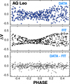 |
Fig. 1. Upper panel: ASAS light curve of AQ Leo folded with 1.615 d, corresponding to the beat period of the FU and FO components of the pulsation. Middle panel: as above, but for the third-order (12-component) Fourier fit given by Eq. (1). Lower panel: residuals of the Fourier fit. |
In this demonstration and throughout this work, we chose the magnitudes obtained by the smallest aperture. The ASAS photometric pipeline uses five aperture sizes, the smallest of which is only 2 pixels wide (i.e., 30″ because of the large field of view of 8.5 ° ×8.5° on a 2K × 2K CCD chip3). Because most of our RRd targets have a low brightness, blending is quite common, especially at larger apertures. Therefore we chose the smallest aperture to minimize the effect of blending on the estimation of the average magnitude (even though other apertures yield light curves of lower scatter).
It is important to ensure that the derived ASAS ⟨V⟩ magnitudes are compatible with high-precision observations. To test this, we relied on the recent compilation of Monson et al. (2017), including both archival data and new observations made by the Three-hundred MilliMeter Telescope (TMMT) of the Carnegie Observatories. By cross-matching their Table 5 and the ASAS archive, we find 22 RRab and 11 RRc stars in common. The ⟨V⟩ magnitudes from these two sources are plotted in Fig. 2. The ASAS photometry does not show any sign of systematic offset for this relatively bright set of objects. The median differences and the mean errors are +0.0017 ± 0.0045 and +0.0029 ± 0.0047 for the FU and FO variables, respectively.
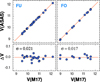 |
Fig. 2. Comparison of the ASAS average ⟨V⟩ magnitudes with those of Monson et al. (2017). Upper panels: ⟨V⟩ vs ⟨V⟩ plots for the FU and FO variables. Lower panels: Monson et al. (2017) ⟨V⟩ minus ASAS ⟨V⟩ as a function of ⟨V⟩ of Monson et al. (2017). Continuous lines indicate levels of equality. |
As mentioned earlier, 26 of the 30 galactic RRd stars in our sample have ASAS data available. For the remaining 4 stars, we should find some way to estimate ⟨V⟩. The obvious choice may seem to be some mixture of the Gaia magnitudes in the three bands. By using the FU/FO variables of Monson et al. (2017), we find that this does not improve the quality of the fit as much as the single-color fit in the BP band alone. Consequently, we used a simple linear transformation of the Gaia EDR3 BP magnitudes to estimate the corresponding flux-averaged V magnitudes. It is important to emphasize that the BP magnitudes used throughout this paper are simple averages (i.e., not the results of Fourier fits). As we show below, for large-amplitude, asymmetric light curves, the transformation will therefore likely yield erroneous estimates for ⟨V⟩.
Eighteen FO variables have precise ⟨V⟩ magnitudes reported by Monson et al. (2017). We added the RRd stars AQ Leo and BS Com to this set because both have non-ASAS-based average V magnitudes (Jerzykiewicz et al. 1982; Dékány al. 2008). Because the published averages for these two stars are magnitude averages, we subtracted 0.015 from the published values to derive a rough estimate on the flux-averaged V magnitude (Bono et al. 1995). We note that for a third RRd star, V0372 Ser, we also have an independent average V magnitude by Benkő & Barcza (2009) that is assumed to be precise. However, their value for some reason appears to disagree both with the ASAS value and with the Gaia-transformed value below. Consequently, we did not use this star in deriving our calibration formula. Finally, we used 20 ⟨V⟩ values in the calibration of the BP magnitudes. Employing a robust least-squares fit, we derived the following formula
 (2)
(2)
Here we subtracted the average of BP over the sample to have uncorrelated errors on the regression coefficients. This transformation leads to a fit with σ = 0.022 mag for the calibrating FO stars.
Figure 3 shows the striking difference between the FU and FO stars. As already mentioned above, this is primarily due to the fact that FU stars have highly nonsinusoidal light variation, and this makes the simple averages (BP average magnitudes) systematically fainter than the Fourier averages. For the RRd stars (lower panel of Fig. 3), a similar effect is observable, but at a much lower level. We note, however, that less severe blending has the same effect, therefore it is difficult to separate the two effects in the present case. For the RRd stars, the overall shift remains in the range of a few hundredths of magnitude for the brighter part of our sample (the item ordering is also brightness ordering for the RRd sample). For fainter stars, the difference between the BP estimated ⟨V⟩ values and those obtained directly from the ASAS data becomes larger and noisier, most likely due to the more severe blend contamination at fainter magnitudes.
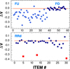 |
Fig. 3. Upper panel: ⟨V⟩ magnitudes of Monson et al. (2017) minus those calculated from the Gaia average BP magnitude (see Eq. (2)). Lower panel: as above, but for the ASAS ⟨V⟩ magnitudes of the RRd stars. Squares show the three outliers whose ⟨V⟩ magnitudes are seriously flawed (most likely by blending) in the ASAS setting. See text for further details. |
We have three strong outliers among the RRd stars. The brightest star, V0381 Tel, indeed has a nearby bright companion, well within the 15″ radius of the smallest aperture used by ASAS. In the case of V0374 Tel, we also have a crowded field with two similarly bright companions some 20″−30″ apart, but it is unclear how they affect the measured brightness of the target if we assume that the 15″ aperture is correctly set. One possibility is that it is positioned on the photocenter of the poorly resolved stellar triplet (target and the nearby companions), and this leads to the higher flux for the target. The faintest star, CF Del, has only 34 data points in the ASAS database, leading to an inaccurate estimate of the average magnitude (the field for this target is also crowded, but the brighter companions are out of the smallest aperture we use).
In summary, according to the analysis presented in this section, we used the Fourier-based flux-averaged magnitudes of the ASAS observations for 23 stars. For the remaining 4 + 3 = 7 stars we estimated ⟨V⟩ from the BP magnitudes of the EDR3 of the Gaia mission. We refer to Table A.1 for the actual values used.
2.2. K magnitudes
The method we employed to derive the parameters of double-mode stars requires knowledge of the effective temperature. The all-sky survey of the WISE infrared satellite (Wright et al. 2010) provides accurate fluxes for all of our targets. Together with the ⟨V⟩ magnitudes (as detailed in Sect. 2.1), we can use one of the numerous V − K → Teff calibrations available in the literature. In order to do this, we need to convert the WISE W1 and W2 magnitudes into K magnitudes (Johnson or 2MASS because they differ only by an additive constant: KJohnson = K2MASS + 0.03)4. We find that the very recent K2MASS flux-averaged magnitudes of nearly 100 galactic field RR Lyrae stars by Layden et al. (2019) and also the very recent catalog of the W1, W2 band-merged fluxes by Schlafly et al. (2019) (the unWISE catalog) suit this task very well.
After some testing, we find that a simple linear formula works well, and further complexities do not lead to any significant improvement. We find that the formula below fits the dereddened 2MASS magnitudes K0 of Layden et al. (2019) with a standard deviation of 0.033 mag,
 (3)
(3)
Here W0 denotes a mixture of the dereddened unWISE magnitudes computed from the published band-merged fluxes and reddening coefficients of Wang & Chen (2019) as follows:
 (4)
(4)
The quality of the calibration of the 98 stars is shown in Fig. 4. The error bars are solely from the errors of the K data because the errors of ∼0.5% from the unWISE catalog are negligible. Except for AR Per, all more substantially deviating stars have large error bars. The outlier status of AR Per might be related to its outstandingly high reddening of E(B − V) = 1.110. Using the extinction ratios of Yuan et al. (2013), which are some 30%–50% higher than those of Wang & Chen (2019), only exacerbates the outlier status of this star. One possibility is that there is a high inhomogeneity in the interstellar matter in the direction of AR Per that happens to become much more transparent in an area that is not resolvable by the instrument on which the map of Schlafly & Finkbeiner (2011) is based. Another (perhaps more likely) possibility is that the foreground extinction is considerably lower than the total extinction given by the reddening map.
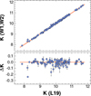 |
Fig. 4. Calibration of the unWISE (Schlafly et al. 2019) W1, W2 magnitudes to the 2MASS K magnitudes of the RR Lyrae sample of Layden et al. (2019). On the vertical axis in the upper panel, we plot dereddened magnitudes K(W1, W2) = K0 (see Eq. (4)). The reference levels are shown by continuous lines, ΔK = K(L19)−K(W1, W2). The strongest outlier in the lower panel is AR Per, with an outstandingly high reddening of E(B − V) = 1.110. |
2.3. Teff(V – K) zeropoint
In our earlier studies (e.g., Kovacs & Walker 1999, hereafter KW99), we used the stellar atmosphere models of Castelli et al. (1997) (hereafter C97) to relate metallicity, gravity, and color to the effective temperature, with the zeropoint (ZP) tied to the generally accepted value based on the infrared flux meethod (IRFM). Here we followed the same method, but updated the zero point by the one given for giants by González Hernández & Bonifacio (2009) (hereafter GB09).
In tying the ZP, we encountered two problems. First, the calibration of GB09 for giants is limited to Teff < 6300 K, with only four points above 6000 K. Therefore the preferred Teff range of ∼6500 − 7000 K of the RRd stars is basically extrapolated when the formula of GB09 is used. Second, the formula of KW99 is linear, whereas that of GB09 is nonlinear, exposing an issue of matching the two calibrations.
The linear formula presented by KW99 matches the C97 models with a residual standard deviation (in log Teff) better than 0.001 (corresponding to 15 − 20 K). The parameter range covered by the fit is as follows: 6000 < Teff < 8000 K, 2.5 < log g < 3.5, −2.5 < [M/H]< − 0.5. Therefore we relied on this high-quality fit concerning the parameter dependence. To match the ZP with that of BG09, we proceeded as follows.
First we chose a set of RR Lyrae stars with reliable V − K colors and metallicities. After testing various selections from the literature, we opted for the abundant sample of Dambis et al. (2013), containing 383 entries with the required number of parameters. To compare the Teff estimates by the KW99 and GB09 formulae, for the KW99 formula we also need to know the gravity. For RR Lyrae stars, the static gravity can be evaluated fairly well even with a limited knowledge of the stellar mass. Using a linear approximation of the type of van Albada & Baker (1971), KW99 derived the following equation from their LNA models:
 (5)
(5)
Without introducing any significant error (at least in the present context), we can fix the stellar mass M at some general value. We used 0.75M⊙ in this particular test.
After computing the two Teff estimates at any given ZP, we obtained a nonlinear dependence of ΔTeff = Teff(GB09)−Teff on Teff due to the nonlinearity of the GB09 formula (see Fig. 5). Here Teff denotes the KW99 fit to the atmosphere models of C97 with the ZP shift of Δlog T0 (see Eq. (7)). To compute the RMS at any given ZP, we need to eliminate the systematic difference that is entirely due to the extrapolation of the GB09 formula from the more populated, low-Teff regime. The correction was made by fitting a second-order correction polynomial to ΔTeff
 (6)
(6)
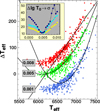 |
Fig. 5. Calibration of the ZP shift Δlog T0 of the Teff formula (Eq. (7)). The vertical axis gives ΔTeff = Teff(GB09)−Teff. The various ridges correspond to the ZP shifts given in the gray boxes. Continuous lines show the correction polynomial (Eq. (6)) at an anchor temperature of Tanc = 6200 K. The inset displays the RMS of the polynomial-corrected residuals as a function of the ZP shift and Tanc (from the bottom up, for Tanc = 6000, 6200, 6400 K). |
We did not have an adjustable constant in the above equation because this is given as a preselected ZP of the KW99 formula (see below). As a result, at the anchor temperature Tanc, no polynomial correction is made to the residual. To test the dependence of ZP on Tanc, we selected three anchors at the tail of the GB09 calibrating sample. The resulting ZPs should be quite independent of the actual values of these anchors.
Our Teff formula with the variable ZP shift of Δlog T0 reads as follows:
![Mathematical equation: $$ \begin{aligned}&\log T_{\rm eff}= 3.9158 - \Delta \log T_0 - 0.1156(V-K) + 0.0069\log {g} \nonumber \\&\qquad \qquad - 0.0026[\mathrm{M/H}], \end{aligned} $$](/articles/aa/full_html/2021/09/aa41100-21/aa41100-21-eq7.gif) (7)
(7)
where V and K are in the Johnson system and reddening free. The metallicity [M/H] was assumed to be solar-scaled, so that ![Mathematical equation: $ [\mathrm{M/H}]=[\mathrm{Fe/H}]=\log Z/Z^{*}_{\odot} $](/articles/aa/full_html/2021/09/aa41100-21/aa41100-21-eq8.gif) , with
, with  5. We recall that KJohnson = K2MASS + 0.03.
For the anchor temperature of 6200, we illustrate the pattern of the temperature difference ΔTeff in Fig. 5. The dots of various colors correspond to the ZP shifts Δlog T0 as indicated in the gray boxes. All correction polynomials are zero at Tanc = 6200 K. For incorrect ZPs, these polynomials provide poor fits to ΔTeff. By scanning the possible ZPs, we obtain with the plot shown in the inset. Independently of the value of Tanc, we conclude with the same ZP shift of 0.0040–0.0055. Finally, we settle at Δlog T0 = 0.0045 in Eq. (7).
2.4. Bolometric correction
Because the theoretical models work with the total irradiated flux, we need to convert the luminosity into the wave-band-limited colors to use the observed magnitudes to constrain the models. This was achieved with the intermediation of the bolometric correction BC, and can be evaluated in various ways. As in our earlier works, we opted for the stellar atmosphere models of C97. For completeness, here we repeat the formula given in KW99 for BC with respect to the Johnson V filter,
![Mathematical equation: $$ \begin{aligned}&\mathrm{BC} = 0.1924 + 0.0633u - 0.0411u^2 - 0.0233u^3 \nonumber \\&\qquad - 0.0464\log {g} + 0.0689f + 0.0118f^2 - 0.0121fu \nonumber \\&f = [\mathrm{M/H}] , \ \ u = c(\log T_{\rm eff} - t) \nonumber \\&c = 2/(\log T_2 - \log T_1) , \ t = (\log T_1 + \log T_2)/2 \nonumber \\&T_1 = 6000 , \ \ T_2 = 8000. \end{aligned} $$](/articles/aa/full_html/2021/09/aa41100-21/aa41100-21-eq10.gif) (8)
(8)
This formula fits the model data with an RMS of 0.001 mag in the parameter range of interest (see Sect. 2.3). We recall that the zeropoint of this formula has been shifted by 0.113 mag with respect to the model values given by the C97 models. With this shift, the models yield BC⊙ = −0.082, which is very close to −0.07, following from the current bolometric and Johnson V magnitudes of the Sun by Willmer (2018). The bolometric magnitude Mbol of the Sun is fixed to 4.74 throughout this paper, also in agreement with Willmer (2018).
To determine the luminosity, we proceeded with the well-known basic formulae,
 (9)
(9)
where the symbols have their standard meanings. The parallax π is given in the units of milliarcsecond [mas].
3. Brief description of the method
The basic idea of using double-mode stars to estimate their physical properties is the same as in our earlier works (e.g., KW99). However, because the targets lack abundance measurements, we need to also involve stellar evolution models, much in the same way as we did in Dékány et al. (2008).
Concerning the pulsation models, we ran a new set of LNA models with a parameter range that was far wider than what is assumed to be occupied by the RRd stars. The model grid covers the full instability strip and beyond. The actual LNA model grid parameters are described in Table 2. All models have 400 mass zones down to 5 × 10⁶ K. Although this number of zones could already provide an accurate estimates both for the period and the growth rates, nearly independently of the zoning, we followed the traditional route of arranging the mass shells that is largely inherited from Stellingwerf (1975) (see also Kovacs & Buchler 1988). This implies placing 80 zones of equal mass from the surface in the hydrogen ionization zone at 11 000 K. The remaining zones have geometrically increasing masses down to our core boundary at 5 × 10⁶ K. The code we used is identical with the code used in our earlier works, that is, all of our models have pure radiative envelopes6 with the diffusion approximation, using the OPAL opacities (Iglesias & Rogers 1996).
Parameter ranges of the pulsation models.
For the stellar evolution input, we chose the recently updated models known as BaSTI7 by Hidalgo et al. (2018). The models we used are horizontal branch (HB) models that allow evolution off the zero-age HB up to the asymptotic giant branch. All models employed in this work are without α element enhancement8, convective overshooting, and diffusion. For a comparison of the grid distributions in the metallicity – mass space, we show these grids for the pulsation and evolutionary models in Fig. 6. Because the topological sensitivity of the evolution tracks at low- to medium masses is high, the evolutionary models are more densely sampled for the mass in this parameter regime. For the pulsation models we do not have this effect, therefore they are uniformly sampled for the mass, whereas taking values near and between the pre-given metallicities by the evolution models.
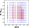 |
Fig. 6. Model metallicities vs mass for the grid values of the BaSTI stellar evolution models (light coral) and the pulsation models (blue) employed in this paper. The metallicities are scaled with Z⊙ = 0.0152 (Caffau et al. 2011). |
Before proceeding with the description of the method of stellar parameter determination, in Fig. 7 we briefly illustrate the position of the 30 galactic RRd stars in the more customary P0–P1/P0 plane (Petersen 1973, 1978). We chose pulsation models sandwiching the metallicity range of the RRd stars to indicate the minimum and maximum metallicities allowed by the observed periods. Without posing further constraints on the pulsation models, the Petersen diagram itself gives only a very rough estimate of the stellar parameters (primarily due to the degeneracy between the metallicity and mass). Still, the arc of the observed RRd stars in the P0–P1/P0 plane clearly indicates the chemical inhomogeneity of the sample. We recall that this pattern was first recognized by the MACHO Collaboration in their work on the multimode RR Lyrae inventory of the Large Magellanic Cloud (Alcock et al. 1997).
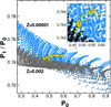 |
Fig. 7. Period – period ratio diagram for the 30 galactic RRd stars (filled yellow circles). The blue and gray dots show two sets of pulsation models for the metallicity labels (corresponding to [M/H] = − 3.18 and −0.88 if Z⊙ = 0.0152). In the main plot, every second model is plotted, whereas in the inset, all models that fit the constrained period regime are shown. |
By using additional (observational and theoretical) pieces of information, we can place further constraints on the LNA models and arrive at a solution for the basic stellar parameters. In brief, we followed the steps below to derive the mass, luminosity, and metallicity for the individual targets.
Set input parameters. The following parameters should be specified: periods of the FU and FO modes, P0 and P1; flux-averaged Johnson V magnitude (or, if it is not available, then Gaia BP magnitude [to be converted into Johnson V via Eq. (2)]); unWISE W1 and W2 fluxes converted to 2MASS K magnitude via Eqs. (3) and (4); reddening E(B − V).
Select pulsation models. Interpolate all available LNA models to the Teff value given by the input parameters and generate dense (M, L) grid from the models by quadratic interpolation on the logarithmic values. Select models satisfying the following period match constraint:
 (10)
(10)
where the upper limit of the logarithmic period distance DPmax is set equal to 0.1%. No interpolation is made to generate a dense metallicity grid. Finally, we obtain a dense (M, L) grid that exactly matches the input temperature at various metallicities and periods satisfying Eq. (10).
Select evolutionary models. Interpolate the stellar evolution tracks linearly to the same temperature as for the pulsation models at any fixed metallicity Z. Then, generate a dense grid by interpolating the (M, L) values corresponding to this fixed temperature. As for the pulsation models, no interpolation is made for the metallicities. We obtain a densely sampled model grid for (M, L) that matches the observed temperature at different metallicities.
Matching pulsational and evolutionary models. For the two (M, L) sets (LNA and HB evolutionary models), we can search for the closest (M, L) pairs at the same metallicity and accept as a solution by minimizing the simple distance measure given by
 (11)
(11)
Iteration on [Fe/H]. Because the metallicity plays a role in estimating the input parameters (i.e., Teff, and therefore log g), we need to iterate the solution to bring the starting metallicity and the one derived via Eq. (11) into close agreement. We find that within about ten iterations, the state of consistency between the input and output metallicities can be reached.
To illustrate the method, we show in Fig. 8 the position of the evolutionary and pulsation models at three different metal abundances for AQ Leo, the prototype of the double-mode RR Lyrae stars. All models have the same Teff of 6595 K as derived from the ASAS V and unWISE W1, W2 magnitudes. The evolutionary and pulsational models exhibit an opposite dependence on the metallicity, enabling a relatively secure selection of the metallicity range in which the iso-Teff curves cross.
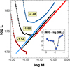 |
Fig. 8. Derivation of the mass, luminosity, and metallicity of AQ Leo from the pulsational and evolutionary models. The labels show the corresponding metallicities, and the color-coding is also applied to the pulsation models. A shift of ±0.003 in log L is used for the pulsation models to clearly show the metallicity effect (no shift for [M/H] = − 1.88, +0.003 and −0.003 for [M/H] = − 2.48 and −1.54, respectively). The inset shows the variation in (M, L) distance metric (Eq. (11)) as a function of the metallicity. All models have the same effective temperature of 6595 K, and the metallicities are scaled with Z⊙ = 0.0152. |
4. Comparison with the Gaia EDR3 luminosities
The early version of the Gaia DR3 enables us to perform a stringent test on the luminosities we derived from the RRd stars. The Gaia luminosities are basically independent of these luminosities because only the bolometric correction contains a dependence on Teff, log g, and [Fe/H] that also enters the evaluation of the RRd luminosities. Errors and RRd solution dependences play a secondary effect in the actual value of the BC.
The RRd luminosities were computed for all the 30 targets as described in Sect. 3. To evaluate the EDR3 luminosities, we added 0.02 mas to the EDR3 parallaxes (see below for some justification of this correction). The luminosities are compared in Fig. 9. All error sources (from BC, ⟨V⟩, and parallax) are included in the vertical error bars shown as 1σ limits for the Gaia luminosities. For the RRd luminosities, the main error source is the ZP of the temperature scale. There are no other observational errors because the periods are very accurate. However, there might be various or unknown errors in the theories we use. Because these errors are difficult to assess precisely enough, and both the evolutionary and the pulsation models proved to be quite accurate in various other applications, we packed all the possible errors in the ZP of Teff, which is known to be somewhat ambiguous. We computed RRd luminosities with log Teff ZPs shifted by ±0.005 with respect to the ZP given in Sect. 2.3. Then, the horizontal error bars in the plot are given as half of the difference between the luminosities obtained with the two extreme log Teff ZPs.
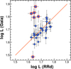 |
Fig. 9. Comparison of the luminosities derived for 30 galactic RRd stars (Tables 1 and A.1) and those computed from the Gaia EDR3 parallaxes. Outliers are marked by squares and are discussed in the text. For reference, the equal-luminosity values are shown by the orange line. |
The two independent sets of luminosities (Gaia and RRd-based) correlate rather remarkably well if we deselect the six outliers marked by red squares. Although parallax errors probably contribute to their outlier status, it is worthwhile to examine other factors such as blending (see also Sect. 2.1). All six objects are found to show various degrees of crowding, at least relative to the resolutions of the instruments contributing to the datasets used9.
Although for CF Del and V0374 Tel we used the transformed Gaia BP magnitudes, their outlier status could not be eliminated. For the remaining four stars (V0458 Her, V5644 Sgr, SW Ret, and XY Crv), we find that the ASAS photometry yields values quite close to the transformed Gaia BP magnitudes, therefore we used the ASAS data. After examining the WISE image stamps10 for the six outliers, we find that the WISE fluxes for SW Ret, XY Crv, and V0374 Tel might have been affected by close companions, if the apertures were shifted toward the photocenters.
In seeking for blend-related cause of the outlier status, it is worthwhile to recall that any systematic change in ⟨V⟩ will affect both the Gaia and the RRd luminosities in a similar way. This is because we use V and K (via the unWISE magnitudes) to estimate Teff. If we increase V (e.g., using Gaia photometry to correct for blending), then we also increase V − K (K remains the same). As a result, Teff becomes lower, yielding a lower luminosity from the RRd analysis (see Fig. 3 of KW99). The higher ⟨V⟩ results in a lower luminosity for the same Gaia parallax. Therefore the status (outlier or not) does not change much by introducing changes in ⟨V⟩. The situation is different if only the infrared fluxes are affected by blending. If corrected for, this will lead to a fainter K magnitude and therefore higher Teff, that is, higher RRd luminosity. This would weaken the outlier status. Unfortunately, this may work only for the three WISE blend candidates listed above. We conclude that the exact underlying cause of the outlier status of these six stars is unclear at this point.
The derived stellar parameters of the 30 RRd stars are displayed in Table 3. The metric used to determine the parameters that yield the closest match of the pulsation and evolutionary models (Eq. (11)) is also given. Eleven stars have a weak matching metric, which means a lack of solution (i.e., lack of crossing the LNA and HBEV curves; see Fig. 8). This issue can be remedied by an increase in Teff ZP11. With a ZP shift of Δlog Teff = +0.005, only three stars have relatively high DML values of 0.01 − 0.02. Only some of the outliers discussed above have this type of low-fidelity solution.
Derived parameters of 30 galactic RRd stars.
Using stellar evolution models with α enhancement may also have some effect on the solution, but it is unlikely that this improves the solution. With the same total heavy element abundance, α enhanced models have lower log L by ∼0.02 (Dorman 1992; VandenBerg et al. 2000). For the pulsation models, the α enhancement also decreases the mass and luminosity at the same level (Kovacs et al. 1992; Kovacs & Walker 1999), therefore the net effect might be rather small.
Considering the ambiguities that still exist in the temperature scale (Boyajian et al. 2013; see, however, Casagrande et al. 2014), it is important to examine how the systematic shift in the Gaia parallax (which appears necessary at this point) changes as we change ZP of Teff. The ZP of the IRFM/GB09-adjusted log Teff scale we used is 3.9113 (see Eq. (7) and subsequent text). We tested three ZP shifts, −0.005, 0.0, and +0.005 with respect to this ZP. For each ZP shift we scanned the average difference between the Gaia and RRd luminosities as a function of the parallax shift with respect to the published EDR3 values. Figure 10 shows that if we accept the ZP dictated by the IRFM work of González Hernández & Bonifacio (2009), then adding 0.02 mas to the published parallaxes can be considered as appropriate to bring the Gaia luminosities into agreement with the RRd luminosities. On the other hand, with an increase of Δlog Teff = 0.005, we may not need to change anything with the EDR3 parallaxes. We recall (as just mentioned) that with a higher temperature scale, the match between the LNA and HBEV models also improves.
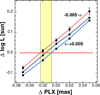 |
Fig. 10. Dependence of the average luminosity difference log(Gaia)−log(RRd) on the parallax shift (published minus shifted) for the RRd star sample. The separate lines correspond to log Teff ZP shifts (relative to our adopted ZP as given in Sect. 2.3) of −0.005, 0.0 and +0.005. Error bars show the statistical errors of the mean differences. To avoid jamming, the error bars are shown only for one Teff ZP shift (others are very similar). The shaded area indicates the range of the allowed EDR3 parallax correction to bring the Gaia and RRd luminosities into agreement. |
Studies of various distance indicators show that the systematic bias in the published Gaia parallaxes decreased at each step of the new releases. From the period-luminosity relation of a large sample of W Uma binaries, Ren et al. (2021) derived that an overall shift of 0.029 mas of the EDR3 parallaxes (i.e., adding 0.029 mas to the published parallaxes) brings them into agreement with those obtained from the standard binary star analyses. The shift differs by only 0.004 mas from the shift suggested by the Gaia team (Lindegren et al. 2021). Using the large sample of benchmark eclipsing binaries of Stassun & Torres (2016), the same authors (Stassun & Torres 2021) drew a similar conclusion, suggesting a somewhat smaller overall shift of 0.025 mas with substantial variation over the ecliptic latitude. The parallax shift derived in this paper favors the above values. However, it is important to emphasize the role of the temperature ZP (as discussed above). Both in the RRd and in the eclipsing binary analyses, a crucial point is the choice of this parameter. A sufficient upward modification may lead to complete agreement, without any parallax shift.
5. PLZ relation from RRd stars
Because the PLZ relations have become increasingly important in the past 20 years in the field of RR Lyrae stars, here we briefly compare the PLZ resulting from the RRd stars derived in this paper for the 2MASS K band and some of the PLZs derived by other means. We note that in a similar comparative work, Dékány (2009) employed 20 RRd stars (3 from the galactic field and 17 from the Large Magellanic Cloud) to compare the Wesenheit indices W(V, B − V) of these stars with those obtained from the Baade-Wesselink (B-W) analysis of 22 galactic FU stars (Kovacs 2003). The conclusion of Dékány (2009) was that the P0–W(V, B − V) relations obtained from the RRd analysis (similar to the one presented in this paper) and from the B-W analysis were statistically consistent. However, the RRd relation was much tighter and steeper than the one resulting from the B-W analysis.
The derivation of the RRd PLZ is very straightforward. The RRd analysis yields P0, Teff, L, and Z. Then, knowing these quantities, we can apply bolometric corrections to the luminosity values and obtain the visual absolute magnitude MV. After inverting Eq. (7) for MV − MK, we obtain the absolute 2MASS K magnitude simply by subtracting 0.03 from MK (see Sect. 2.2).
The resulting log P0–Ks plot (where Ks denotes the 2MASS K magnitude) is shown in the upper panel of Fig. 11. As expected, the correlation is significant, but the scatter is somewhat excessive. It has long been claimed and shown in several papers (e.g., Bono et al. 2003) that the metallicity dependence for Ks is also significant. The lower panel of Fig. 11 shows that by regressing both the period and metallicity, we obtain a considerably tighter correlation. With three relatively mild outliers (XX Crv, AZ For, and AG PsA), a robust fit yields the following formula:
![Mathematical equation: $$ \begin{aligned}&K_s=-(0.396\pm 0.003) - (2.606\pm 0.134)(\log P_0 + 0.30) \nonumber \\&\qquad +(0.158\pm 0.011)([\mathrm{Fe/H}]+1.36). \end{aligned} $$](/articles/aa/full_html/2021/09/aa41100-21/aa41100-21-eq14.gif) (12)
(12)
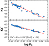 |
Fig. 11. Upper panel: absolute Ks magnitudes derived from pulsation and evolution models for the 30 galactic RRd stars of Table 1 as a function of the fundamental period. Lower panel: as above, but for the modified Ks values for the metallicity effect. Continuous lines show the respective regressions (see Eq. (12) for the fit shown in the lower panel). |
The standard deviation of this regression is 0.0086 mag. It is interesting to examine the Teff ZP issue discussed in Sect. 4 in terms of the tightness of the RRd PLZ relation. The tightness of this relation apparently fairly significantly favors the GB09 scale. By changing the ZP of log Teff for the three-parameter fits, we obtain residual standard deviations of 0.025 and 0.043 magnitudes for Δlog Teff = −0.005 and +0.005, respectively. This result seems to contradict the higher temperature scale suggested by the better HBEV/LNA match accuracy of the models and further supports the need for a correction of the Gaia parallaxes12. Nevertheless, it is unclear how tight the true PLZ should be. There is a hidden mass and temperature dependence in the PLZ relation, and it is not entirely known how strongly evolutionary and color effects cause a correlation of these parameters with each other, and thereby tighten the observed PLZ relation.
In a comparison with other recent variants of the RR Lyrae PLZ relation, we chose the relation of Marconi et al. (2015), based on pulsation and stellar evolution considerations, and that of Neeley et al. (2019) from the purely empirical fit to the bright single-mode RR Lyrae stars with high-fidelity Gaia (DR2) parallaxes. The PLZ relations are compared in Fig. 12. The agreement is very good between all these independent estimates, with a tighter but systematically more deviating trend for the relation based on the Gaia DR2 parallaxes. In a comparison of the regression coefficients (see Table 4), we see that although our formula seems to be closer to that of Neeley et al. (2019), the systematic trend is stronger than for the formula of Marconi et al. (2015). This underlines the significance of the metallicity term, which is stronger in both of these formulae than in ours. This is partially compensated for by the weaker period dependence in the formula of Marconi et al. (2015), but works in the opposite way with the strong period dependence derived by Neeley et al. (2019). In spite of these details, which are likely due to the errors of the fits, the overall agreement with standard deviations of 0.005–0.01 mag is very satisfying between the different approximations.
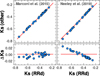 |
Fig. 12. Comparison of the PLZ relations as given in Table 4. All formulae are compared on the set of (log P0, [Fe/H]) values given in Table 3. The lower panels show the differences ΔKs = Ks(RRd)−Ks(other) between the pair of formulae. |
Comparison of the PLZ regression coefficient.
6. Conclusions
The steadily improving accuracy of the Gaia parallaxes allows us to visit an increasing number of objects and derive various physical parameters with impressively high precision. RR Lyrae stars come into the forefront of investigation together with other objects because they are significant in galactic structure and stellar evolution. We used relatively bright galactic double-mode RR Lyrae (RRd) stars and compared their (largely) theoretical luminosities with those obtained (almost) directly from their parallaxes that are currently made available by the third (early) data release (EDR3) of the Gaia mission. With almost all individual parallax errors smaller than 10% and a sample size of 30, it is possible to aim for a statistical precision of a few percent in defining the zeropoint of the RR Lyrae luminosity scale and investigate the source of the remaining systematic differences.
We implemented a method that is very similar to methods used in our earlier investigations. The method is based on the simple observation that the two periods yield a closed solution for the stellar parameters, assuming that we have reliable estimates on the temperature and metallicity. Unfortunately, this quantity is unavailable for the stars we studied here, therefore we resorted to the combination of pulsation and evolutionary models (BaSTI, Hidalgo et al. 2018), together with observationally determined temperature much in the same way as in Dékány et al. (2008). In return, this method yielded a full solution, including an estimate on the metallicity. Our main results are listed below.
-
Except for 6 outlying stars (likely affected by blending and parallax errors), the luminosities of the remaining 24 stars correlate well with those derived from the Gaia EDR3 parallaxes.
-
By fixing the Teff zeropoint to the one given by González Hernández & Bonifacio (2009), we obtain no systematic differences between the Gaia and RRd luminosities, assuming that the Gaia parallaxes are shifted by 0.02 mas upward. This result agrees with other studies that suggested similar (but higher than some 0.005–0.01 mas) corrections.
-
We derived a PLZ relation for the 2MASS K color and found that it agrees well with two other independent PLZ relations. The first relation (Neeley et al. 2019) is based on direct Gaia DR2 distances, whereas the second (Marconi et al. 2015) comes from pulsation-stellar evolution considerations. Our PLZ relation is fundamentally theoretical, aided by the observationally calibrated zeropoint of Teff. There are no significant differences in the PLZ ZPs, and the predicted values have a scatter (standard deviation) of only ∼0.01 mag.
-
The tightness criterion of the RRd PLZ relation significantly favors the Teff zeropoint accepted for this study. This lends further support to the upward correction of the EDR3 parallaxes, as mentioned above.
The work presented in this paper would have been much simpler and independent of stellar evolutionary models if reliable metal abundances were available for our targets. When the metallicity and temperature are known, the luminosity can be estimated using only pulsation theory, and these values can be directly compared with the Gaia luminosities without the intermediary of the evolutionary models. The future availability of metallicity for bright double-mode variables, and, in particular, for RR Lyrae stars, is an important step for a nearly direct test of the Gaia parallaxes and evolutionary models.
Assuming that the Hertzsprung progression (Hertzsprung 1926) is caused by the 2 : 1 resonance between the fundamental and second-overtone modes, as first suggested by Simon & Schmidt (1976) and confirmed by several subsequent studies, e.g., by Buchler et al. (1990).
See https://old.ipac.caltech.edu/2mass/releases/second/doc/sec6_3.html, counterchecked for this paper by inspection of the data used in Liu & Janes (1989, 1990).
The C97 models refer to the available or accepted solar heavy element abundance. We therefore mark Z⊙ with an asterisk.
Without the capability of modeling sustained double-mode pulsation, the relevance of using periods from nonlinear convective models instead of those from linear radiative models cannot be quantified.
Bag of Stellar Tracks and Isochrones, http://basti-iac.oa-abruzzo.inaf.it/index.html
Some discussion of the effect of α enhancement can be found in Sect. 4.
The resolution limits for ASAS, WISE, and Gaia are 15″, ∼6″, and ∼2″, respectively. See Sect. 2.1 and Lindegren et al. (2021) and Ren et al. (2021).
The temperature increase shifts the LNA lines to higher values in the M–L plane with an opposite effect on the HBEV curves, leading to a better chance for intersecting.
In a current paper on single-mode galactic RR Lyrae stars, Marconi et al. (2021) concluded that the parallax correction might be statistically insignificant. However, their data appear to be too noisy to detect the small parallax shift claimed by other studies.
Acknowledgments
It is a pleasure to thank to Andy Monson for the valuable correspondence on the calibration of the photometric data used in this paper. This work is based heavily on the availability of well-calibrated photometry of the All Sky Automated Survey (ASAS). We thank to Grzegorz Pojmanski and his co-workers for running this great project for so many years. This research has made use of the VizieR catalogue access tool, CDS, Strasbourg, France (DOI: 10.26093/cds/vizier). This work has made use of data from the European Space Agency (ESA) mission Gaia (https://www.cosmos.esa.int/gaia), processed by the Gaia Data Processing and Analysis Consortium (DPAC, https://www.cosmos.esa.int/web/gaia/dpac/consortium). Funding for the DPAC has been provided by national institutions, in particular the institutions participating in the Gaia Multilateral Agreement. This publication makes use of data products from the Wide-field Infrared Survey Explorer, which is a joint project of the University of California, Los Angeles, and the Jet Propulsion Laboratory/California Institute of Technology, funded by the National Aeronautics and Space Administration. This research has made use of the NASA/IPAC Infrared Science Archive, which is funded by the National Aeronautics and Space Administration and operated by the California Institute of Technology. This research has made use of the International Variable Star Index (VSX) database, operated at AAVSO, Cambridge, Massachusetts, USA. Supports from the National Research, Development and Innovation Office (grants K 129249 and NN 129075) are acknowledged.
References
- Alcock, C., Allsman, R. A., Alves, D., et al. 1997, ApJ, 482, 89 [NASA ADS] [CrossRef] [Google Scholar]
- Benkő, J. M., & Barcza, Sz. 2009, A&A, 497, 481 [Google Scholar]
- Bernhard, K., & Wils, P. 2006, IBVS, 5698 [Google Scholar]
- Blazhko, S. 1907, Astron. Nachr., 175, 325 [NASA ADS] [CrossRef] [Google Scholar]
- Bono, G., Caputo, F., & Stellingwerf, R. F. 1995, ApJS, 99, 263 [NASA ADS] [CrossRef] [Google Scholar]
- Bono, G., Caputo, F., Castellani, V., et al. 2003, MNRAS, 344, 1097 [Google Scholar]
- Boyajian, T. S., von Braun, K., van Belle, G., et al. 2013, ApJ, 771, 40 [NASA ADS] [CrossRef] [Google Scholar]
- Buchler, J. R., Moskalik, P., & Kovacs, G. 1990, ApJ, 351, 617 [NASA ADS] [CrossRef] [Google Scholar]
- Caffau, E., Ludwig, H.-G., Steffen, M., et al. 2011, Sol. Phys., 268, 255 [NASA ADS] [CrossRef] [Google Scholar]
- Casagrande, L., Portinari, L., Glass, I. S., et al. 2014, MNRAS, 439, 2060 [Google Scholar]
- Castelli, F., Gratton, R. G., & Kurucz, R. L. 1997, A&A, 318, 841 [NASA ADS] [Google Scholar]
- Clementini, G., Di Tomaso, S., Di Fabrizio, L., et al. 2000, AJ, 120, 2054 [NASA ADS] [CrossRef] [Google Scholar]
- Cox, A. N. 1991, ApJ, 381, L71 [NASA ADS] [CrossRef] [Google Scholar]
- Cox, A. N., Hodson, S. W., & Clancy, S. P. 1983, ApJ, 266, 94 [NASA ADS] [CrossRef] [Google Scholar]
- Dambis, A. K., Berdnikov, L. N., Kniazev, A. Y., et al. 2013, MNRAS, 435, 3206 [Google Scholar]
- Dékány, I. 2009, AIPC, 1170, 245 [Google Scholar]
- Dékány, I., Kovacs, G., Jurcsik, J., et al. 2008, MNRAS, 386, 521 [NASA ADS] [CrossRef] [Google Scholar]
- Dorman, B. 1992, ApJS, 81, 221 [NASA ADS] [CrossRef] [Google Scholar]
- Dziembowski, W. A. 2016, CoKon, 105, 23 [Google Scholar]
- Garcia-Melendo, E., & Clement, Ch. M. 1997, AJ, 114, 1190 [NASA ADS] [CrossRef] [Google Scholar]
- Garcia-Melendo, E., Henden, A. A., & Gomez-Forrellad, J. M. 2001, IBVS, 5167 [Google Scholar]
- González Hernández, J. I., & Bonifacio, P. J. I. 2009, A&A, 497, 497 [NASA ADS] [CrossRef] [EDP Sciences] [Google Scholar]
- Hertzsprung, E. 1926, Bull. Astr. Inst. Neth., 3, 115 [NASA ADS] [Google Scholar]
- Hidalgo, S. L., Pietrinferni, A., Cassisi, S., et al. 2018, ApJ, 856, 125 [Google Scholar]
- Iglesias, C. A., & Rogers, F. J. 1991, ApJ, 371, L73 [NASA ADS] [CrossRef] [Google Scholar]
- Iglesias, C. A., & Rogers, F. J. 1996, ApJ, 464, 943 [NASA ADS] [CrossRef] [Google Scholar]
- Jerzykiewicz, M., & Wenzel, W. 1977, Acta Astron., 27, 35 [NASA ADS] [Google Scholar]
- Jerzykiewicz, M., Schult, R. H., & Wenzel, W. 1982, Acta Astron., 32, 358 [NASA ADS] [Google Scholar]
- Jurcsik, J., Smitola, P., Hajdu, G., et al. 2015, ApJS, 219, 25 [CrossRef] [Google Scholar]
- Kolláth, Z., Buchler, J. R., Szabó, R., et al. 2002, A&A, 385, 932 [NASA ADS] [CrossRef] [EDP Sciences] [Google Scholar]
- Koppelman, M. D., Wils, P., Welch, D. L., Durkee, R., & Vidal-Sáinz, J. 2004, in American Astronomical Society Meeting 205, id. 54.05, Bull. Am. Astron. Soc., 36, 1428 [Google Scholar]
- Kovacs, G. 2000a, A&A, 360, L1 [NASA ADS] [Google Scholar]
- Kovacs, G. 2000b, A&A, 363, L1 [NASA ADS] [Google Scholar]
- Kovacs, G. 2003, MNRAS, 342, L58 [NASA ADS] [CrossRef] [Google Scholar]
- Kovacs, G., & Buchler, J. R. 1988, ApJ, 324, 1026 [NASA ADS] [CrossRef] [Google Scholar]
- Kovacs, G., & Buchler, J. R. 1993, ApJ, 404, 765 [NASA ADS] [CrossRef] [Google Scholar]
- Kovacs, G., & Walker, A. R. 1999, ApJ, 512, 271 [NASA ADS] [CrossRef] [Google Scholar]
- Kovacs, G., Buchler, J. R., & Marom, A. 1991, A&A, 252, L27 [NASA ADS] [Google Scholar]
- Kovacs, G., Buchler, J. R., Marom, A., et al. 1992, A&A, 259, L46 [Google Scholar]
- Layden, A. C., Tiede, G. P., Chaboyer, B., et al. 2019, AJ, 158, 105 [NASA ADS] [CrossRef] [Google Scholar]
- Lindegren, L., Klioner, S. A., Hernández, J., et al. 2021, A&A, 649, A2 [EDP Sciences] [Google Scholar]
- Liu, T., & Janes, K. A. 1989, ApJS, 69, 593 [NASA ADS] [CrossRef] [Google Scholar]
- Liu, T., & Janes, K. A. 1990, ApJ, 354, 273 [NASA ADS] [CrossRef] [Google Scholar]
- McClusky, J. V. 2008, IBVS, 5825 [Google Scholar]
- Marconi, M., Coppola, G., Bono, G., et al. 2015, ApJ, 808, 50 [Google Scholar]
- Marconi, M., Molinaro, R., Ripepi, V., et al. 2021, MNRAS, 500, 5009 [Google Scholar]
- Monson, A. J., Beaton, R. L., Scowcroft, V., et al. 2017, AJ, 153, 96 [NASA ADS] [CrossRef] [Google Scholar]
- Moskalik, P., & Kolaczkowski, Z. 2009, MNRAS, 394, 1649 [NASA ADS] [CrossRef] [Google Scholar]
- Neeley, J. R., Marengo, M., Freedman, W. L., et al. 2019, MNRAS, 490, 4254 [Google Scholar]
- Oosterhoff, P. Th. 1957a, Bull. Astron. Inst. Neth., 13, 317 [NASA ADS] [Google Scholar]
- Oosterhoff, P. Th. 1957b, Bull. Astron. Inst. Neth., 13, 320 [NASA ADS] [Google Scholar]
- Petersen, J. O. 1973, A&A, 27, 89 [NASA ADS] [Google Scholar]
- Petersen, J. O. 1978, A&A, 62, 205 [NASA ADS] [Google Scholar]
- Pilecki, B., & Szczygiel, D. M. 2007, IBVS, 5785 [Google Scholar]
- Pojmanski, G. 1997, Acta Astron., 47, 467 [Google Scholar]
- Preston, G. W. 1959, ApJ, 130, 507 [NASA ADS] [CrossRef] [Google Scholar]
- Ren, F., Chen, X., Zhang, H., et al. 2021, ApJ, 911, L20 [NASA ADS] [CrossRef] [Google Scholar]
- Schlafly, E. F., & Finkbeiner, D. P. 2011, ApJ, 737, 103 [NASA ADS] [CrossRef] [Google Scholar]
- Schlafly, E. F., Meisner, A. M., & Green, G. M. 2019, ApJS, 240, 30 [Google Scholar]
- Seaton, M. J., Yan, Y., Mihalas, D., et al. 1994, MNRAS, 266, 805 [NASA ADS] [CrossRef] [Google Scholar]
- Simon, N. R. 1982, ApJ, 260, L87 [Google Scholar]
- Simon, N. R., & Schmidt, E. 1976, ApJ, 205, 162 [NASA ADS] [CrossRef] [Google Scholar]
- Smolec, R., & Moskalik, P. 2010, A&A, 524, A40 [NASA ADS] [CrossRef] [EDP Sciences] [Google Scholar]
- Smolec, R., Dziembowski, W., Moskalik, P., et al. 2017, EPJWC, 152, 06003 [NASA ADS] [Google Scholar]
- Stassun, K. G., & Torres, G. 2016, ApJ, 831, L6 [NASA ADS] [CrossRef] [Google Scholar]
- Stassun, K. G., & Torres, G. 2021, ApJ, 907, L33 [NASA ADS] [CrossRef] [Google Scholar]
- Stellingwerf, R. F. 1975, ApJ, 195, 441 [NASA ADS] [CrossRef] [Google Scholar]
- Stobie, R. S. 1977, MNRAS, 180, 631 [NASA ADS] [CrossRef] [Google Scholar]
- Szczygiel, D. M., & Fabrycky, D. C. 2007, MNRAS, 377, 1263 [NASA ADS] [CrossRef] [Google Scholar]
- van Albada, T. S., & Baker, N. 1971, ApJ, 169, 311 [NASA ADS] [CrossRef] [Google Scholar]
- VandenBerg, D. A., Swenson, F. J., Rogers, F. J., et al. 2000, ApJ, 532, 430 [NASA ADS] [CrossRef] [Google Scholar]
- Wang, S., & Chen, X. 2019, ApJ, 877, 116 [NASA ADS] [CrossRef] [Google Scholar]
- Willmer, C. N. A. 2018, ApJS, 236, 47 [NASA ADS] [CrossRef] [Google Scholar]
- Wils, P. 2006, IBVS, 5685 [Google Scholar]
- Wils, P. 2010, IBVS, 5955 [Google Scholar]
- Wils, P., & Otero, S. A. 2005, IBVS, 5593 [Google Scholar]
- Wils, P., Lloyd, C., & Bernhard, K. 2006, MNRAS, 368, 1757 [NASA ADS] [CrossRef] [Google Scholar]
- Wright, E. L., Eisenhardt, P. R. M., Mainzer, A. K., et al. 2010, AJ, 140, 1868 [Google Scholar]
- Yuan, H. B., Liu, X. W., & Xiang, M. S. 2013, MNRAS, 430, 2188 [NASA ADS] [CrossRef] [Google Scholar]
Appendix A: Observational datasets
We summarize the observational data we used in Table A.1. The discoveries and periods were reported in the papers listed in Table 1.
Observed properties of 30 Galactic RRd stars.
The flux-averaged magnitudes in the Johnson V filter are based on the third-order Fourier fit (see Sect. 2.1) to the ASAS V observations by starting from the published periods and refining them iteratively. This step was necessary because of the long time span of the ASAS data. Four entries (marked by double asterisks) do not have ASAS light curves, therefore their ⟨V⟩ values were approximated with the aid of the Gaia photometry as described in Sect. 2.1. The same procedure was employed on three more stars (V0381 Tel, V0374 Tel, and CF Del), where blending and sparse light-curve sampling corrupted the ASAS magnitudes.
For completeness, the flux-averaged Gaia EDR3 magnitudes are listed for all three bands, even though we only used the BP magnitudes. For the ASAS ⟨V⟩ values, we assumed a flat error of 0.005 mag for all entries, whereas for those derived from the Gaia average fluxes, we give the errors as given by the EDR3 catalog.
The W1, W2 fluxes come from the recent unWISE catalog by Schlafly et al. (2019) and result from the band-integrated fluxes throughout the full mission of the satellite. The reddening values are from the map of Schlafly & Finkbeiner (2011), which is accessible from the NASA/IPAC Infrared Science Archive. Parallaxes are from the Gaia EDR3 catalog (accessed from the VizieR database).
All Tables
All Figures
|
Fig. 1. Upper panel: ASAS light curve of AQ Leo folded with 1.615 d, corresponding to the beat period of the FU and FO components of the pulsation. Middle panel: as above, but for the third-order (12-component) Fourier fit given by Eq. (1). Lower panel: residuals of the Fourier fit. |
| In the text | |
|
Fig. 2. Comparison of the ASAS average ⟨V⟩ magnitudes with those of Monson et al. (2017). Upper panels: ⟨V⟩ vs ⟨V⟩ plots for the FU and FO variables. Lower panels: Monson et al. (2017) ⟨V⟩ minus ASAS ⟨V⟩ as a function of ⟨V⟩ of Monson et al. (2017). Continuous lines indicate levels of equality. |
| In the text | |
|
Fig. 3. Upper panel: ⟨V⟩ magnitudes of Monson et al. (2017) minus those calculated from the Gaia average BP magnitude (see Eq. (2)). Lower panel: as above, but for the ASAS ⟨V⟩ magnitudes of the RRd stars. Squares show the three outliers whose ⟨V⟩ magnitudes are seriously flawed (most likely by blending) in the ASAS setting. See text for further details. |
| In the text | |
|
Fig. 4. Calibration of the unWISE (Schlafly et al. 2019) W1, W2 magnitudes to the 2MASS K magnitudes of the RR Lyrae sample of Layden et al. (2019). On the vertical axis in the upper panel, we plot dereddened magnitudes K(W1, W2) = K0 (see Eq. (4)). The reference levels are shown by continuous lines, ΔK = K(L19)−K(W1, W2). The strongest outlier in the lower panel is AR Per, with an outstandingly high reddening of E(B − V) = 1.110. |
| In the text | |
|
Fig. 5. Calibration of the ZP shift Δlog T0 of the Teff formula (Eq. (7)). The vertical axis gives ΔTeff = Teff(GB09)−Teff. The various ridges correspond to the ZP shifts given in the gray boxes. Continuous lines show the correction polynomial (Eq. (6)) at an anchor temperature of Tanc = 6200 K. The inset displays the RMS of the polynomial-corrected residuals as a function of the ZP shift and Tanc (from the bottom up, for Tanc = 6000, 6200, 6400 K). |
| In the text | |
|
Fig. 6. Model metallicities vs mass for the grid values of the BaSTI stellar evolution models (light coral) and the pulsation models (blue) employed in this paper. The metallicities are scaled with Z⊙ = 0.0152 (Caffau et al. 2011). |
| In the text | |
|
Fig. 7. Period – period ratio diagram for the 30 galactic RRd stars (filled yellow circles). The blue and gray dots show two sets of pulsation models for the metallicity labels (corresponding to [M/H] = − 3.18 and −0.88 if Z⊙ = 0.0152). In the main plot, every second model is plotted, whereas in the inset, all models that fit the constrained period regime are shown. |
| In the text | |
|
Fig. 8. Derivation of the mass, luminosity, and metallicity of AQ Leo from the pulsational and evolutionary models. The labels show the corresponding metallicities, and the color-coding is also applied to the pulsation models. A shift of ±0.003 in log L is used for the pulsation models to clearly show the metallicity effect (no shift for [M/H] = − 1.88, +0.003 and −0.003 for [M/H] = − 2.48 and −1.54, respectively). The inset shows the variation in (M, L) distance metric (Eq. (11)) as a function of the metallicity. All models have the same effective temperature of 6595 K, and the metallicities are scaled with Z⊙ = 0.0152. |
| In the text | |
|
Fig. 9. Comparison of the luminosities derived for 30 galactic RRd stars (Tables 1 and A.1) and those computed from the Gaia EDR3 parallaxes. Outliers are marked by squares and are discussed in the text. For reference, the equal-luminosity values are shown by the orange line. |
| In the text | |
|
Fig. 10. Dependence of the average luminosity difference log(Gaia)−log(RRd) on the parallax shift (published minus shifted) for the RRd star sample. The separate lines correspond to log Teff ZP shifts (relative to our adopted ZP as given in Sect. 2.3) of −0.005, 0.0 and +0.005. Error bars show the statistical errors of the mean differences. To avoid jamming, the error bars are shown only for one Teff ZP shift (others are very similar). The shaded area indicates the range of the allowed EDR3 parallax correction to bring the Gaia and RRd luminosities into agreement. |
| In the text | |
|
Fig. 11. Upper panel: absolute Ks magnitudes derived from pulsation and evolution models for the 30 galactic RRd stars of Table 1 as a function of the fundamental period. Lower panel: as above, but for the modified Ks values for the metallicity effect. Continuous lines show the respective regressions (see Eq. (12) for the fit shown in the lower panel). |
| In the text | |
|
Fig. 12. Comparison of the PLZ relations as given in Table 4. All formulae are compared on the set of (log P0, [Fe/H]) values given in Table 3. The lower panels show the differences ΔKs = Ks(RRd)−Ks(other) between the pair of formulae. |
| In the text | |
Current usage metrics show cumulative count of Article Views (full-text article views including HTML views, PDF and ePub downloads, according to the available data) and Abstracts Views on Vision4Press platform.
Data correspond to usage on the plateform after 2015. The current usage metrics is available 48-96 hours after online publication and is updated daily on week days.
Initial download of the metrics may take a while.