| Issue |
A&A
Volume 653, September 2021
|
|
|---|---|---|
| Article Number | A90 | |
| Number of page(s) | 11 | |
| Section | Stellar atmospheres | |
| DOI | https://doi.org/10.1051/0004-6361/202140979 | |
| Published online | 13 September 2021 | |
Exploiting the Gaia EDR3 photometry to derive stellar temperatures
1
Dipartimento di Fisica e Astronomia Augusto Righi, Università degli Studi di Bologna,
Via Gobetti 93/2,
40129
Bologna,
Italy
e-mail: This email address is being protected from spambots. You need JavaScript enabled to view it.
2
INAF – Osservatorio di Astrofisica e Scienza dello Spazio di Bologna,
Via Gobetti 93/3,
40129
Bologna,
Italy
3
University of Groningen, Kapteyn Astronomical Institute,
9747
AD
Groningen,
The Netherlands
Received:
1
April
2021
Accepted:
3
June
2021
Abstract
We present new colour–effective temperature (Teff) transformations based on the photometry of the early third data release (EDR3) of the ESA/Gaia mission. These relations are calibrated on a sample of about 600 dwarf and giant stars for which Teff has previously been determined with the infrared flux method from dereddened colours. The 1σ dispersion of the transformations is of 60–80 K for the pure Gaia colours (BP−RP)0, (BP−G)0, and (G−RP)0, improving to 40–60 K for colours including the 2MASS Ks-band, namely (BP−Ks)0, (RP−Ks)0, and (G−Ks)0. We validate these relations in the most challenging case of dense stellar fields, where the Gaia EDR3 photometry could be less reliable, providing guidance for the safe use of Gaia colours in crowded environments. We compare the Teff from the Gaia EDR3 colours with those obtained from standard (V−Ks)0 colours for stars in three Galactic globular clusters of different metallicity, namely NGC 104, NGC 6752, and NGC 7099. The agreement between the two estimates of Teff is excellent, with mean differences of between –50 and +50 K, depending on the colour, and with 1σ dispersions around the mean Teff differences of 25–50 K for most of the colours and below 10 K for (BP−Ks)0 and (G−Ks)0. This demonstrates that these colours are analogous to (V−Ks)0 as Teff indicators.
Key words: stars: fundamental parameters / stars: atmospheres / techniques: photometric
© ESO 2021
1 Introduction
Effective temperatures (Teff) for FGK-spectral type stars can be estimated with different methods either based directly on the stellar spectra, for example the wings of the Balmer lines, the line–depth ratio, and the excitation equilibrium, or on the photometric properties. The infrared flux method (IRFM, Blackwell & Shallis 1977; Blackwell et al. 1979, 1980) is one of the most popular methods based on photometric colours, requiring accurate and precise photometry (especially for the infrared spectral range) and knowledge of the colour excess, E(B – V). Several implementations of this method have been presented in the literature (see e.g. Alonso et al. 1999; Ramírez & Meléndez 2005; González Hernández & Bonifacio 2009; Casagrande et al. 2010). Teff derived with this method for suitable calibrators is also used to obtain relations between different broad-band colours and Teff, enabling an immediate estimate of Teff even for stars for which the IRFM cannot be directly used.
The ESA/Gaia mission (Gaia Collaboration 2016) is providing accurate and precise all-sky photometry in three broad-band photometric filters, named G, BP, and RP. Gaia DR2 colour–Teff transformations calibrated on IRFM Teff have been presented by Mucciarelli & Bellazzini (2020, MB20 hereafter) and Casagrande et al. (2021).
The recent Gaia Early Data Release 3 (EDR3, Gaia Collaboration 2021) has significantly improved upon the previous DR2, including astrometric and photometric information for about 1.5 billion stars. The superior quality of Gaia EDR3 photometry and its internal homogeneity (Yang et al. 2021; Riello et al. 2020, R20 hereafter) guarantees further improvement in the determination of stellar parameters. In this paper we present new colour–Teff transformations based on Gaia EDR3 and 2MASS photometry, validating these relations in the case of crowded stellar fields.
2 New colours–Teff transformations
Following the same procedure adopted in MB20, we derived colour–Teff transformations for differentbroad-band colours including the Gaia passbands. We used the IRFM Teff computed by González Hernández & Bonifacio (2009) for a sample of about 450 dwarf stars (log g > 3.0) and about 200 giant stars (log g < 3.0) with metallicity between [Fe/H] ~−4.0 and 0.0 dex. The broad-band colours that we considered in the analysis are  ,
,  ,
,  ,
,  ,
,  and
and  . These were derived adopting the Gaia EDR3 photometry (Gaia Collaboration 2021) and the Ks -band magnitudes from the Two Micron All Sky Survey (2MASS, Skrutskie et al. 2006). Gaia magnitudes have been corrected for interstellar reddening following the iterative procedure described in Gaia Collaboration (2018), while Ks magnitudes have been corrected adopting the extinction coefficient by McCall (2004). Colour excess values E(B − V) are the same as those used by González Hernández & Bonifacio (2009).
We computed the best polynomial fit relating each colour C with θ (defined as θ = 5040/Teff) and the stellar metallicity [Fe/H], according to the functional form:
![Mathematical equation: \begin{equation*}\theta\,{=}\,{b_0}+{b_1}{C}+{b_2}{C^2}+{b_3}\textrm{[Fe/H]}+{b_4}{\textrm{[Fe/H]}^2}+{b_5}\textrm{[Fe/H]}{C},\end{equation*}](/articles/aa/full_html/2021/09/aa40979-21/aa40979-21-eq16.png) (1)
(1)
and considering dwarf and giant stars separately. A few outliers have been removed adopting an iterative 2.5σ-clipping procedure. Table 1 lists the colour range of validity, the number of stars used for the fit, the 1σ dispersion of the fit residuals, and the coefficients b0, …, b5, for both dwarf and giant stars samples.
The colour–Teff relations that we obtained in this way have typical 1σ dispersion of ~40–60 K and ~40–80 K, for dwarf and giant stars, respectively. The 1σ dispersion of the relations is usually adopted as a conservative estimate of the uncertainty in the derived Teff when this kind of colour–Teff relation is provided and/or used (see e.g. Alonso et al. 1999; González Hernández & Bonifacio 2009; Casagrande et al. 2021). This uncertainty should be added in quadrature to that obtained by propagating the error on colour. The uncertainty in [Fe/H] has a negligible impact on the derived Teff, as a variation of ±0.1 dex leads to a change in Teff of smaller than ~10 K, depending on the adopted relation. Finally, we verified that the temperature differences given by the relations for dwarfs and giants at the adopted dwarf–giant threshold (log g = 3.0) is about 10–20 K, significantly smaller than the uncertainties.
In the common practice of abundance analysis, a full propagation of the errors, including errors in the relation coefficients, is not adopted (we are not aware of a single example in the literature for the field of stellar population studies). The uncertainties involved in the whole process of abundance estimates are so many and so deeply entangled that a full propagation can be prone to underestimation of the actual errors on the abundances. However, for application cases requiring full error propagation on the final Teff estimates, in Appendix B we provide (a) alternative relations adopting differences with respect to the mean colour as an independent variable (e.g. using 
 , instead of
  alone) to minimise the off-diagonal terms of the covariance matrix, and (b) the full covariance matrices for all the relations.
The new transformations are very similar to those provided by MB20 based on Gaia DR2 photometry, reflecting the similarity between the DR2 and EDR3 photometric systems. The use of the old relations with Gaia EDR3 photometry provides Teff that differ by less than 40–50 K from those obtained with the new relations. Also, the new transformations have 1σ dispersion similar to or smaller than those obtained with DR2 photometry. In particular, we noted that the dispersions of all of the transformations including the G-band magnitudes are reduced by ~20–30% with respectto those obtained with Gaia DR2 photometry. Indeed, according to R20, the most significant improvements between DR2 and EDR3 photometry occurred in the bright star regime that is spanned by our calibrating sources (G <6.0).
FiguresA.1–A.6 show the colour–Teff trends for the adopted calibrating sample and the corresponding polynomial fit. The stars are coloured according to the metallicity interval they belong to: [Fe/H] ≤−2.5 dex (blue points),−2.5 < [Fe/H] ≤−1.5 (green points), − 1.5 < [Fe/H] ≤−0.5 (red points), [Fe/H] > −0.5 dex (black points). Finally, Fig. A.7 shows the behaviour of the fit residuals as a function of [Fe/H] for all the relations.
We compared the predictions of the Casagrande et al. (2021) relations with ours for the stars of our calibrating sample, using all the colours that can be obtained by combining the three Gaia pass-bands and then also combining these with 2MASS K. The mean differences are within ≃ ± 100 K and the scatter is small (spanning ≲50 K) in all cases except for the  colour, where dwarfs display a mean difference of about 250 K and a significant scatter (≳100 K). Taking into account that part of the observed differences may be due to the subtle changes between Gaia DR2 and EDR3 photometry (especially for G ≤ 13.0, see Evans et al. 2018, R20), we can conclude that the two calibrations provide consistent results within the uncertainties. The Casagrande et al. (2021) relations use 14 coefficients and explicitly include the dependency on surface gravity; they may therefore be appropriate when all the astrophysical parameters of the target stars, except Teff, are already known with high accuracy. On the other hand, our relations account for the very small effect of surface gravity by means of a simple giant–dwarf dichotomy and are defined by just five parameters; they are simpler and have a wider range of applicability in most real cases.
Coefficients b0,...,b5 of the colour–Teff relations.
3 Application on three globular clusters: NGC 104, NGC 6752, M 30
The new relations are based on isolated bright field stars for which Gaia provides superb photometry that is usually not affected by issues related to stellar contamination and/or background subtraction. To test the effectiveness of our relations in determining reliable Teff in any condition, we decided to validate them in dense stellar fields, where the superior photometric quality of the Gaia magnitudes can be hampered by the high stellar crowding.
The selected stellar fields with which we perform such a test correspond to three Galactic globular clusters (GCs), namely NGC 104 (47 Tucanae), NGC 6752, and NGC 7099 (M 30). These were selected according to the following criteria:
They must span the entire range of metallicity covered by the population of Galactic clusters, with the selection of a metal-rich GC [NGC 104, Fe/H] = –0.75 dex), a metal-intermediate GC (NGC 6752, [Fe/H] = –1.49 dex), and a metal-poor GC (NGC 7099, [Fe/H] = –2.31 dex) according to the iron abundances derived by Mucciarelli & Bonifacio (2020). The reason behind the choice of clusters with different [Fe/H] is to check the validity of our transformations against the metallicity, because this parameter enters our Eq. (1) directly;
They must have a low colour excess E(B – V) (between 0.04 and 0.07 mag, see Mucciarelli & Bonifacio 2020) in order to minimise the effect of uncertainties in the extinction on the derivation of Teff;
They must have available ground-based V photometry from the database maintained by P. B. Stetson (Stetson et al. 2019) and Ks -band photometry from 2MASS Skrutskie et al. (2006). This is to derive a reference Teff using homogeneous
 colours.
Clusters members were first selected to have proper motions within 1.5 mas yr−1 (for NGC 104 and NGC 6752) and 1.0 mas yr−1 (for NGC 7099) from the cluster mean proper motions as given by Baumgardt et al. (2019). Then we filtered stars based on ‘goodness of measure’ EDR3 quality parameters, following prescriptions provided byLindegren et al. (2018) and R20, including in our final samples only stars with: (i) ruwe < 1.4; and (ii) ∣C*∣ < 2σc, where C* and σc are defined according to Eq. (6) and (18), respectively, in R20.
For these cluster stars we computed Teff adopting the six colour–Teff transformations derived in Sect. 2. Additionally, reference Teff were computed using the  -Teff transformation by González Hernández & Bonifacio (2009). The latter is based on the same sample of stars and IRFM Teff used to derived our own relations, and therefore all these Teff are on the same scale. We restricted this analysis to the stars with G < 17 and with error in
  smaller than 0.03 mag in order to exclude stars with large uncertainties in the 2MASS Ks magnitudes. To be sure that the different fitting procedures used here for the Gaia colours and used by González Hernández & Bonifacio (2009) for
  do not introduce systematic errors in the computed Teff, we derived the
  -Teff transformation adopting our procedure and the
  already used by González Hernández & Bonifacio (2009). The average difference in the Teff from the two
  -Teff transformations for the cluster stars is of +1 K (σ = 6 K). Hence, our fitting procedure does not introduce differences with respect to the transformations by González Hernández & Bonifacio (2009) and we can compare Teff from Gaia and
  colours.
From the results of our analysis, it is clear that there are advantages and disadvantages to using each of the photometric colours as a Teff indicator, because of the different wavelength baseline and their sensitivity to Teff, and other parameters, such as metallicity and surface gravity. Here we adopt Teff from the  colour as reference values to check the robustness of those derived from Gaia EDR3 photometry. The
  colour is one of the most common and reliable photometric indicators of Teff (see e.g. Fernley 1989; Bessell et al. 1998; Alonso et al. 1999) because of two main factors:
- (i)
the different sensitivity to Teff of the flux in V - and Ks -bands. This effect is clearly visible in Fig. 1, which shows a set of synthetic fluxes with Teff from 4000 to 6000 K in steps of 250 K. All the synthetic spectra have been calculated with the SYNTHE spectral synthesis code (Kurucz 2005). The V-band flux is highly sensitive to Teff, increasing by a factor of ten as Teff ranges from 4000 to 6000 K. On the other hand, the Ks-band flux increases by only a factor of 1.5 in spite of the same Teff change. Therefore,
 effectively behaves as the ratio between a Teff-sensitive flux and an almost Teff-insensitive flux. (ii) The Johnson–Cousins V band photometry is better standardised than other optical bands, for example the B and I bands, whose definitions can vary depending on the adopted photometric system (Bessell & Brett 1988).
Figure 2 shows the behaviour of the differences between Teff from Gaia EDR3 colours and from  as a function of the latter for the stars in the three GCs. The average values of these differences, the corresponding 1σ dispersion, and number of stars are listed in Table 2.
Teff from pure Gaia EDR3 colours have mean differences with respect to the reference Teff of between +20 and +50 K, with scatter between 25 and 50 K. In the case of the metal-rich GC NGC 104 a mild trend of ΔTeff with the reference Teff exists, in the sense that the Gaia EDR3 Teff becomes slightly hotter than those from  for the coldest stars.
The colours including Ks magnitudes show small average differences and 1σ dispersions; in particular,  and
and  provide the best agreement with the Teff from
  , with 1σ dispersions smaller than 10 K. This simple test demonstrates that:
(Gaia-Ks) colours are analogous to
 as Teff indicators because they have a large wavelength baseline including filters with different sensitivity in Teff;
the calibrations based on field (isolated) stars also work well in crowding conditions typical of nearby Galactic GCs (D≲10.0 kpc) once the simple selections based on quality parameters described above are adopted (see below, for further discussion).
4 How to derive accurate Teff in crowded stellar fields
The use of the Gaia EDR3 photometry to infer Teff in dense stellarfields (like globular clusters) needs a note of caution because the Gaia magnitudes, regardless of their formal small uncertainties, can be affected by issues concerning the background subtraction and contamination by neighbouring stars (R20).
The left panels of Fig. 3 show the three colour–magnitude diagrams for NGC 104 including pure Gaia colours. At variance with  , the other two colours show an asymmetric broadening of the red giant branch (RGB) that becomes more evident for G > 14. In particular, an excess of stars bluer than the main locus of the RGB is visible when we use
  , while with
  the situation is the opposite, with an excess of redder stars. These anomalous colours translate to anomalous Teff that can be as discrepant as ±500 K compared to RGB stars with the same G magnitude. Indeed, BP and RP magnitudes are known to be more prone than G magnitudes to contamination from light not related to the target sources (e.g. nearby stars), for reasons inherent to the different way in which BP/RP and G fluxes are acquired and processed (R20).
Stars with anomalous colours can be easily identified and excluded by applying the criterion used in Sect. 2 for the three target clusters (∣C*∣ < 2σc). In Fig. 3 the sources fulfilling this criterion (therefore considered as high-quality/reliable photometry sources) are shown as red circles, while those excluded are shown as grey circles. This exercise provides three important results. (i) The criterion ∣ C* ∣ < 2σc allows us to efficiently identify stars with possible issues related to background subtraction and stellar contamination; (ii) Furthermore, this procedure is essential whether  or
or  are used; only reliable sources provide reliable Teff while the other sources significantly over- or under-estimate (for
  and
and  , respectively) Teff. (iii) Lastly the symmetrical effect observed in
  and
and  (and in the corresponding Teff) is largely cancelled out when
  is adopted. Indeed,
  of reliable and contaminated stars provide indistinguishable Teff.
In conclusion, according to this limited set of experiments, reliable Teff in (non-extreme) crowded fields can be obtained by removing stars with corrupted colours with criteria based on quality parameters provided in the Gaia source catalogue. The criterion proposed here (∣ C*∣ < 2σc) is simple and very effective in the considered cases, but there may be cases where only stars not fulfilling such criteria are available for the analysis. The results presented above suggest that reliable Teff estimates can also obtained for these stars using  as Teff an indicator, and taking advantage of the fact that BP and RP magnitudes are similarly affected by any light contamination entering the aperture window of BP and RP spectrophotometry (see R20, for a discussion on this subject).
 |
Fig. 1 Main panel: synthetic spectra calculated with Teff from 4000 K (spectrum with the lower flux) to 6000 K (spectrum with the higher flux) in steps of 250 K. All the spectra adopt [M/H] = –1.0 dex. The upper panel shows the profile of the photometric filters used in this work. |
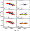 |
Fig. 2 Differences between Teff derived from the Gaia colours and from |


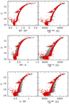 |
Fig. 3 Colour-magnitude diagrams for NGC 104 considering the pure Gaia colours (left panels) and the corresponding Teff vs. G-band magnitudes diagrams (right panels). Red and grey points mark the stars selected and rejected according to the criterion provided by R20, respectively. The horizontal lines in the right panels mark the transition between the dwarf and giant star regimes. |
Average differences between Teff derived from the Gaia EDR3 colours and  for the globular clusters NGC 104, NGC 6752, and NGC 7099.
5 The impact of the Gaia Teff on the chemical abundances
As a sanity check, we evaluated the impact of the new colour–Teff transformations derived from Gaia EDR3 photometry on the chemical abundances from high-resolution spectra. We consider the data set of high-resolution spectra acquired with the spectrograph UVES at the Very Large telescope of ESO for giant stars in 16 Galactic GCs already analysed by Mucciarelli & Bonifacio (2020). The iron abundance of these stars were derived following the same procedure adopted by Mucciarelli & Bonifacio (2020) and using the new Teff scales. These new [Fe/H] values were compared with those obtained for the same stars from  by Mucciarelli & Bonifacio (2020).
In the case of pure Gaia colours, the new Teff are comparable with those from  , with differences smaller than100 K. These new Teff lead to higher [Fe/H], with differences of between 0.01 and 0.05 dex with respect to the values obtained from
  Teff. Figure 4 shows, as an example, the difference in the derived [Fe/H] when adopting Teff from
  or
or  . The average [Fe/H] difference is +0.03 dex (σ = 0.01 dex). The Gaia colours including Ks magnitudes provide a value of Teff for the spectroscopic targets that is almost indistinguishable from the one from
  , such that the average impact in terms of [Fe/H] is smaller than 0.01 dex. We conclude that the use of Teff from Gaia EDR3 photometry leads to chemical abundances that are fully consistent with those obtained adopting Teff from standard colours.
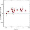 |
Fig. 4 Behaviour of |


6 Conclusions
We exploited the Gaia EDR3 photometry to derive new colour–Teff transformations based on theIRFM Teff provided by González Hernández & Bonifacio (2009) for a sample of about 600 bright dwarf and giant field stars. These transformations have typical uncertainties of 40–80 K and 40–60 K for giant and dwarf stars, respectively. We checked the validity of these transformations in the case of GC stars, where the superior photometric quality of the Gaia magnitudes can be hampered by the high stellar crowding, providing guidelines for safe estimates of Teff in these cases. In summary, the Gaia EDR3 photometry can be safely used to derive precise and accurate Teff with the following recommendations:
When reliable Ks-band photometry is available, mixed colours (Gaia–Ks) should be preferred, as they display the maximum sensitivity to temperature. In particular,
 and
and
 are the best choices because their colour–Teff transformation shows the smallest dispersion and the best agreement with Teff derived from
  ;
;When Ks-band photometry is not available or is not sufficiently precise, pure Gaia colours can be used to derive Teff, althoughthey show slightly larger dispersion with respect to the broad band colours including Ks;
BP- and RP-band magnitudes in crowded fields can be affected by issues concerning stellar blending and background subtraction, despite their high photometric precision. For this reason,
 and
and
 can lead to under- and over-estimated Teff, respectively. To avoid these effects, stars should be selected according to C* and we recommend the criterion ∣C*∣ < 2σc. Alternatively,
  should be preferred over other combinations of Gaia magnitudes, because the effects of contamination from light not related to the target source are similar in the BP and RP bands and almost cancel out when subtracted.
Acknowledgements
We thank the referee, Floor van Leeuwen, for the comments and suggestions that improved the manuscript. We also thank Paolo Montegriffo for the useful discussions. This work has made use of data from the European Space Agency (ESA) mission Gaia (https://www.cosmos.esa.int/gaia), processed by the Gaia Data Processing and Analysis Consortium (DPAC, https://www.cosmos.esa.int/web/gaia/dpac/consortium). Funding for the DPAC has been provided by national institutions, in particular the institutions participating in the Gaia Multilateral Agreement. This research has made extensive use of the R programming language and R Studio environment.
Appendix A Colour-Teff polynomial fits
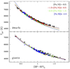 |
Fig. A.1 Behaviour of Teff derived from IRFM by González Hernández & Bonifacio (2009) as a function of the
|


 |
Fig. A.7 Behaviour of the temperature residuals as a function of [Fe/H] for all the colour–Teff transformations discussed in this work. Colours are the same as in previous figures. |
Appendix B An alternative set of colour–Teff transformations
As explained in Section 2, the usual approach to estimate the uncertainty in Teff derived from colour–Teff transformations is to propagate the colour error, sometimes adding in quadrature the 1σ dispersion of the fit residuals taken as a conservative estimate of the relation error. An appropriate propagation of the errors, including the uncertainties on the fit parameters and their possible covariance terms, is nevertheless provided in the following, by means of an alternative set of colour–Teff transformations obtained with following fitting formula (reducing the off-diagonal terms of the covariance matrix):
![Mathematical equation: \begin{equation*}\theta = {\textrm{c}_0}+{\textrm{c}_1}{\textrm{C}^*}+{\textrm{c}_2}{\textrm{C}^{*2}}+{\textrm{c}_3}{\textrm{[Fe/H]}^*}+{\textrm{c}_4}{\textrm{[Fe/H]}^{*2}}+{\textrm{c}_5}{\textrm{[Fe/H]}^*}{\textrm{C}^*},\end{equation*}](/articles/aa/full_html/2021/09/aa40979-21/aa40979-21-eq62.png) (B.1)
(B.1)
where C* is the colour subtracted by the mean colour and [Fe/H]* is the metallicity subtracted by the mean metallicity. Table 2 lists the coefficients ci and the mean colour for each transformation (for all of them we assume –1.5 dex as mean metallicity). The 1σ dispersion and the number of used stars are the same listed in Table 1.
For a given pair of colour–metallicity, the relations 1 and B.1 (and the corresponding coefficients) provide exactly the same results. Relation 1 is more direct to use without needing to scale both colour and metallicity to the mean values used of the calibrators sample. It can be used when the 1σ dispersion of the fit is assumed as reliable estimate of the Teff error due to the calibration itself. Relation B.1 needs the scaling of both colour and metallicity to the mean values used of the calibrators sample and should be used when the user is interested in calculating the Teff uncertainty by propagating also the errors in the coefficients.
We list the normalised covariance matrix for each transformation. In each matrix, the raws and the columns correspond to the parameters c0, c1, c2, c3, c4 and c5, in this order.
(BP-RP)0 - dwarf stars
![Mathematical equation: \[\left[\begin{array}{rrrrrr} 1.000 & 0.045 & -0.229 & -0.034 & -0.503 & 0.075\\ 0.008 & 1.000 & -0.288 & -0.414 & 0.359 & -0.699\\ -0.021 & -0.288 & 1.000 & -0.012 & -0.114 & -0.198\\ -0.035 & -0.414 & -0.012 & 1.000 & -0.615 & 0.350\\ -0.583 & 0.359 & -0.114 & -0.615 & 1.000 & -0.400\\ 0.017 & -0.699 & -0.198 & 0.350 & -0.400 & 1.000\\ \end{array} \right] \]](/articles/aa/full_html/2021/09/aa40979-21/aa40979-21-eq63.png)
(BP-RP)0 - giant stars
![Mathematical equation: \[\left[\begin{array}{rrrrrr} 1.000 & -0.070 & -0.335 & 0.001 & -0.651 & -0.013\\ -0.024 & 1.000 & 0.110 & -0.281 & 0.056 & -0.387\\ -0.050 & 0.110 & 1.000 & -0.342 & -0.124 & 0.108\\ 0.003 & -0.281 & -0.342 & 1.000 & 0.281 & -0.050\\ -1.252 & 0.056 & -0.124 & 0.281 & 1.000 & -0.279\\ -0.005 & -0.387 & 0.108 & -0.050 & -0.279 & 1.000\\ \end{array} \right] \]](/articles/aa/full_html/2021/09/aa40979-21/aa40979-21-eq64.png)
-
 - dwarf stars
![Mathematical equation: \[\left[\begin{array}{rrrrrr} 1.000 & -0.079 & -0.175 & 0.018 & -0.578 & 0.192\\ -0.007 & 1.000 & -0.416 & -0.330 & 0.331 & -0.597\\ -0.004 & -0.416 & 1.000 & 0.032 & -0.061 & -0.272\\ 0.020 & -0.330 & 0.032 & 1.000 & -0.580 & 0.215\\ -0.679 & 0.331 & -0.061 & -0.580 & 1.000 & -0.401\\ 0.022 & -0.597 & -0.272 & 0.215 & -0.401 & 1.000\\ \end{array} \right] \]](/articles/aa/full_html/2021/09/aa40979-21/aa40979-21-eq66.png)
-
 - giant stars
![Mathematical equation: \[\left[\begin{array}{rrrrrr} 1.000 & 0.068 & -0.340 & -0.067 & -0.638 & -0.046\\ 0.012 & 1.000 & 0.222 & -0.432 & 0.039 & -0.391\\ -0.014 & 0.222 & 1.000 & -0.293 & -0.081 & -0.018\\ -0.115 & -0.432 & -0.293 & 1.000 & 0.193 & 0.223\\ -1.238 & 0.039 & -0.081 & 0.193 & 1.000 & -0.301\\ -0.010 & -0.391 & -0.018 & 0.223 & -0.301 & 1.000\\ \end{array} \right] \]](/articles/aa/full_html/2021/09/aa40979-21/aa40979-21-eq68.png)
-
 - dwarf stars
![Mathematical equation: \[\left[\begin{array}{rrrrrr} 1.000 & 0.137 & -0.268 & -0.085 & -0.435 & -0.052\\ 0.014 & 1.000 & -0.136 & -0.498 & 0.368 & -0.774\\ -0.006 & -0.136 & 1.000 & -0.033 & -0.144 & -0.102\\ -0.084 & -0.498 & -0.033 & 1.000 & -0.641 & 0.459\\ -0.514 & 0.368 & -0.144 & -0.641 & 1.000 & -0.404\\ -0.006 & -0.774 & -0.102 & 0.459 & -0.404 & 1.000\\ \end{array} \right] \]](/articles/aa/full_html/2021/09/aa40979-21/aa40979-21-eq70.png)
-
 - giant stars
![Mathematical equation: \[\left[\begin{array}{rrrrrr} 1.000 & -0.226 & -0.345 & 0.060 & -0.630 & 0.019\\ -0.038 & 1.000 & -0.001 & -0.074 & 0.077 & -0.400\\ -0.012 & -0.001 & 1.000 & -0.434 & -0.161 & 0.238\\ 0.100 & -0.074 & -0.434 & 1.000 & 0.354 & -0.349\\ -1.263 & 0.077 & -0.161 & 0.354 & 1.000 & -0.256\\ 0.004 & -0.400 & 0.238 & -0.349 & -0.256 & 1.000\\ \end{array} \right] \]](/articles/aa/full_html/2021/09/aa40979-21/aa40979-21-eq72.png)
-
 - dwarf stars
![Mathematical equation: \[\left[\begin{array}{rrrrrr} 1.000 & 0.098 & -0.243 & -0.073 & -0.425 & -0.035\\ 0.041 & 1.000 & -0.205 & -0.451 & 0.386 & -0.805\\ -0.118 & -0.205 & 1.000 & -0.013 & -0.181 & -0.026\\ -0.068 & -0.451 & -0.013 & 1.000 & -0.678 & 0.435\\ -0.471 & 0.386 & -0.181 & -0.678 & 1.000 & -0.393\\ -0.018 & -0.805 & -0.026 & 0.435 & -0.393 & 1.000\\ \end{array} \right] \]](/articles/aa/full_html/2021/09/aa40979-21/aa40979-21-eq74.png)
-
 - giant stars
![Mathematical equation: \[\left[\begin{array}{rrrrrr} 1.000 & -0.021 & -0.313 & -0.038 & -0.680 & -0.064\\ -0.015 & 1.000 & 0.135 & -0.278 & 0.037 & -0.499\\ -0.246 & 0.135 & 1.000 & -0.358 & -0.111 & 0.133\\ -0.067 & -0.278 & -0.358 & 1.000 & 0.262 & -0.001\\ -1.327 & 0.037 & -0.111 & 0.262 & 1.000 & -0.206\\ -0.055 & -0.499 & 0.133 & -0.001 & -0.206 & 1.000\\ \end{array} \right] \]](/articles/aa/full_html/2021/09/aa40979-21/aa40979-21-eq76.png)
-
 - dwarf stars
![Mathematical equation: \[\left[\begin{array}{rrrrrr} 1.000 & -0.182 & -0.122 & 0.012 & -0.531 & 0.197\\ -0.040 & 1.000 & -0.434 & -0.222 & 0.382 & -0.761\\ -0.018 & -0.434 & 1.000 & -0.003 & -0.228 & 0.035\\ 0.012 & -0.222 & -0.003 & 1.000 & -0.648 & 0.179\\ -0.601 & 0.382 & -0.228 & -0.648 & 1.000 & -0.335\\ 0.061 & -0.761 & 0.035 & 0.179 & -0.335 & 1.000\\ \end{array} \right] \]](/articles/aa/full_html/2021/09/aa40979-21/aa40979-21-eq78.png)
-
 - giant stars
![Mathematical equation: \[\left[\begin{array}{rrrrrr} 1.000 & -0.021 & -0.315 & -0.033 & -0.688 & -0.081\\ -0.008 & 1.000 & 0.176 & -0.271 & 0.054 & -0.512\\ -0.077 & 0.176 & 1.000 & -0.346 & -0.094 & 0.169\\ -0.060 & -0.271 & -0.346 & 1.000 & 0.226 & 0.054\\ -1.353 & 0.054 & -0.094 & 0.226 & 1.000 & -0.176\\ -0.038 & -0.512 & 0.169 & 0.054 & -0.176 & 1.000\\ \end{array} \right] \]](/articles/aa/full_html/2021/09/aa40979-21/aa40979-21-eq80.png)
-
 - dwarf stars
![Mathematical equation: \[\left[\begin{array}{rrrrrr} 1.000 & 0.166 & -0.225 & -0.111 & -0.407 & -0.116\\ 0.056 & 1.000 & -0.102 & -0.457 & 0.328 & -0.823\\ -0.068 & -0.102 & 1.000 & -0.028 & -0.206 & -0.018\\ -0.105 & -0.457 & -0.028 & 1.000 & -0.663 & 0.448\\ -0.468 & 0.328 & -0.206 & -0.663 & 1.000 & -0.341\\ -0.050 & -0.823 & -0.018 & 0.448 & -0.341 & 1.000\\ \end{array} \right] \]](/articles/aa/full_html/2021/09/aa40979-21/aa40979-21-eq82.png)
-
 - giant stars
![Mathematical equation: \[\left[\begin{array}{rrrrrr} 1.000 & -0.057 & -0.323 & -0.013 & -0.680 & -0.072\\ -0.031 & 1.000 & 0.136 & -0.220 & 0.035 & -0.502\\ -0.147 & 0.136 & 1.000 & -0.383 & -0.114 & 0.200\\ -0.023 & -0.220 & -0.383 & 1.000 & 0.277 & -0.070\\ -1.344 & 0.035 & -0.114 & 0.277 & 1.000 & -0.175\\ -0.046 & -0.502 & 0.200 & -0.070 & -0.175 & 1.000\\ \end{array} \right] \]](/articles/aa/full_html/2021/09/aa40979-21/aa40979-21-eq84.png)
References
- Alonso, A., Arribas, S., & Martinez-Roger, C. 1999 A&AS, 140, 261 [NASA ADS] [CrossRef] [EDP Sciences] [Google Scholar]
- Baumgardt, H., Hilker, M., Sollima, A., et al. 2019, MNRAS, 482, 5138 [Google Scholar]
- Bessell, M. S., & Brett, J. M. 1988, PASP, 100, 1134 [NASA ADS] [CrossRef] [Google Scholar]
- Bessell, M. S., Castelli, F., & Plez, B. 1998, A&A, 333, 231 [NASA ADS] [Google Scholar]
- Blackwell, D. E., & Shallis, M. J. 1977, MNRAS, 180, 177 [NASA ADS] [CrossRef] [Google Scholar]
- Blackwell, D. E., Shallis, M. J., & Selby, M. J. 1979, MNRAS, 188, 847 [NASA ADS] [CrossRef] [Google Scholar]
- Blackwell, D. E., Petford, A. D., & Shallis, M. J. 1980, A&A, 82, 249 [NASA ADS] [Google Scholar]
- Casagrande, L., Ramírez, I., Meléndez, J., Bessell, M., & Asplund, M. 2010, A&A, 512, A54 [NASA ADS] [CrossRef] [EDP Sciences] [Google Scholar]
- Casagrande, L., Lin, J., Rains, A. D., et al. 2021, MNRAS, 507, 2684 [NASA ADS] [CrossRef] [Google Scholar]
- Evans, D. W., Riello, M., De Angeli, F., et al. 2018, A&A, 616, A4 [NASA ADS] [CrossRef] [EDP Sciences] [Google Scholar]
- Fernley, J. A. 1989, MNRAS, 239, 905 [NASA ADS] [CrossRef] [Google Scholar]
- Gaia Collaboration (Prusti, T., et al.) 2016, A&A, 595, A1 [NASA ADS] [CrossRef] [EDP Sciences] [Google Scholar]
- Gaia Collaboration (Babusiaux, et al) 2018, A&A, 616, A10 [NASA ADS] [CrossRef] [EDP Sciences] [Google Scholar]
- Gaia Collaboration (Brown, A. G. A., et al) 2021, A&A, 649, A1 [NASA ADS] [CrossRef] [EDP Sciences] [Google Scholar]
- González Hernández, J. I., & Bonifacio, P. 2009, A&A, 497, 497 [NASA ADS] [CrossRef] [EDP Sciences] [Google Scholar]
- Kurucz, R. L. 2005, Mem. Soc. Astron. Ital. Suppl., 8, 14 [Google Scholar]
- Lindegren, L., Hernández, J., Bombrun, A., et al. 2018, A&A, 616, A2 [NASA ADS] [CrossRef] [EDP Sciences] [Google Scholar]
- McCall, M. L. 2004, AJ, 128, 2144 [NASA ADS] [CrossRef] [Google Scholar]
- Mucciarelli, A., & Bellazzini, M. 2020, Res. Notes Am. Astron. Soc., 4, 52 [CrossRef] [Google Scholar]
- Mucciarelli, A., & Bonifacio, P. 2020, A&A, 640, A87 [CrossRef] [EDP Sciences] [Google Scholar]
- Ramírez, I., & Meléndez, J. 2005, ApJ, 626, 446 [Google Scholar]
- Riello, M., De Angeli, F., Evans, D. W., et al. 2021, A&A, 649, A3 [NASA ADS] [CrossRef] [EDP Sciences] [Google Scholar]
- Skrutskie, M. F., Cutri, R. M., Stiening, R., et al. 2006, AJ, 131, 1163 [NASA ADS] [CrossRef] [Google Scholar]
- Stetson, P. B., Pancino, E., Zocchi, A., et al. 2019, MNRAS, 485, 3042 [NASA ADS] [CrossRef] [Google Scholar]
- Yang, L., Yuan, H., Zhang, R., et al. 2021, ApJ, 908, L24 [NASA ADS] [CrossRef] [Google Scholar]
All Tables
Average differences between Teff derived from the Gaia EDR3 colours and for the globular clusters NGC 104, NGC 6752, and NGC 7099.
All Figures
|
Fig. 1 Main panel: synthetic spectra calculated with Teff from 4000 K (spectrum with the lower flux) to 6000 K (spectrum with the higher flux) in steps of 250 K. All the spectra adopt [M/H] = –1.0 dex. The upper panel shows the profile of the photometric filters used in this work. |
| In the text | |
|
Fig. 2 Differences between Teff derived from the Gaia colours and from |
| In the text | |
|
Fig. 3 Colour-magnitude diagrams for NGC 104 considering the pure Gaia colours (left panels) and the corresponding Teff vs. G-band magnitudes diagrams (right panels). Red and grey points mark the stars selected and rejected according to the criterion provided by R20, respectively. The horizontal lines in the right panels mark the transition between the dwarf and giant star regimes. |
| In the text | |
|
Fig. 4 Behaviour of |
| In the text | |
|
Fig. A.1 Behaviour of Teff derived from IRFM by González Hernández & Bonifacio (2009) as a function of the
|
| In the text | |
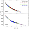 |
Fig. A.2 Same as Fig. A.1 but for the |
| In the text | |
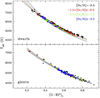 |
Fig. A.3 Same as Fig. A.1 but for the |
| In the text | |
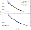 |
Fig. A.4 Same as Fig. A.1 but for the |
| In the text | |
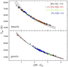 |
Fig. A.5 Same as Fig. A.1 but for the |
| In the text | |
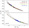 |
Fig. A.6 Same as Fig. A.1 but for the |
| In the text | |
|
Fig. A.7 Behaviour of the temperature residuals as a function of [Fe/H] for all the colour–Teff transformations discussed in this work. Colours are the same as in previous figures. |
| In the text | |
Current usage metrics show cumulative count of Article Views (full-text article views including HTML views, PDF and ePub downloads, according to the available data) and Abstracts Views on Vision4Press platform.
Data correspond to usage on the plateform after 2015. The current usage metrics is available 48-96 hours after online publication and is updated daily on week days.
Initial download of the metrics may take a while.