| Issue |
A&A
Volume 653, September 2021
|
|
|---|---|---|
| Article Number | A131 | |
| Number of page(s) | 18 | |
| Section | The Sun and the Heliosphere | |
| DOI | https://doi.org/10.1051/0004-6361/202140872 | |
| Published online | 23 September 2021 | |
Effects of ambipolar diffusion on waves in the solar chromosphere
Centre for mathematical Plasma Astrophysics, KU Leuven, 3001 Leuven, Belgium
e-mail: This email address is being protected from spambots. You need JavaScript enabled to view it.
Received:
24
March
2021
Accepted:
20
May
2021
Abstract
Context. The chromosphere is a partially ionized layer of the solar atmosphere that mediates the transition between the photosphere where the gas motion is determined by the gas pressure and the corona dominated by the magnetic field.
Aims. We study the effect of partial ionization for 2D wave propagation in a gravitationally stratified, magnetized atmosphere characterized by properties that are similar to those of the solar chromosphere.
Methods. We adopted an oblique uniform magnetic field in the plane of propagation with a strength that is suitable for a quiet sun region. The theoretical model we used is a single fluid magnetohydrodynamic approximation, where ion-neutral interaction is modeled by the ambipolar diffusion term. Magnetic energy can be converted into internal energy through the dissipation of the electric current produced by the drift between ions and neutrals. We used numerical simulations in which we continuously drove fast waves at the bottom of the atmosphere. The collisional coupling between ions and neutrals decreases with the decrease in the density and the ambipolar effect thus becomes important.
Results. Fast waves excited at the base of the atmosphere reach the equipartition layer and are reflected or transmitted as slow waves. While the waves propagate through the atmosphere and the density drops, the waves steepen into shocks.
Conclusions. The main effect of ambipolar diffusion is damping of the waves. We find that for the parameters chosen in this work, the ambipolar diffusion affects the fast wave before it is reflected, with damping being more pronounced for waves which are launched in a direction perpendicular to the magnetic field. Slow waves are less affected by ambipolar effects. The damping increases for shorter periods and greater magnetic field strengths. Small scales produced by the nonlinear effects and the superposition of different types of waves created at the equipartition height are efficiently damped by ambipolar diffusion.
Key words: Sun: chromosphere / waves / methods: numerical / Sun: magnetic fields / Sun: oscillations
© ESO 2021
1. Introduction
Ambipolar diffusion is the dissipation of the magnetic field through the electric field created by the drift velocity between neutrals and charged particles. It is the most important process of magnetic field decay in neutron stars (Jones 1987; Hoyos et al. 2010; Sinha 2020). Ambipolar diffusion has significant effects on turbulence present in the interstellar medium (Brandenburg 2019) or as produced by the magnetorotational instability in weakly ionized disks (Bai & Stone 2011). In the solar context, ambipolar diffusion makes an important contribution to the chromosphere. The chromosphere is the layer of the solar atmosphere that hosts the transition between the almost neutral photosphere to the fully ionized corona. As the density drops with height, the neutrals and the charged particles become incompletely coupled by collisions in the chromosphere.
Waves are ubiquitous in the solar atmosphere and have been observed at different layers from the photosphere to the corona. Because of the limitation on the spatial and temporal resolution of current telescopes, only low-frequency waves have been observed thus far. However, theoretical computations of Musielak et al. (1994) for the acoustic flux generated by the solar convection showed a peak located among the high-frequency waves, corresponding to periods of ≈10 s. These are the waves we study in this paper.
In a single-fluid magnetohydrodynamic (MHD) approach, the interaction between neutrals and charges is assumed to happen on a timescale much shorter than the hydrodynamic timescale. The effect of ion-neutral interactions can be introduced as a contribution to the electric field in a generalized Ohm’s law. This is different from a full two-fluid model, where there are separate equations which describe the time evolution of neutrals and charges, so that there is no assumption about their collisional timescale. It has been shown that in many situations, the single fluid MHD (extended with ambipolar terms) and the full two-fluid treatment give very similar results (Brandenburg 2019; Popescu Braileanu 2020).
In the solar context, mode conversion from fast to Alfvén waves has been studied by taking into account the effect of ambipolar diffusion (Cally & Khomenko 2018). This conversion from fast magneto-acoustic modes to Alfvén modes happens for large periods. It has been shown that this mode conversion is not significantly modified by ambipolar diffusion, but only indirectly affected through the damping of the fast waves. The overall conclusion is that the main effect of ambipolar diffusion is damping of waves (Cally & Khomenko 2018). In this paper, we study a purely 2D configuration where the Alfvén waves are omitted, but we also take a detailed look at how slow and fast mode propagation is affected by ambipolar diffusion.
Waves that are excited by convection motions in the photosphere propagate upwards, and they split into fast and slow components at the equipartition layer where the sound speed is similar to the Alfvén speed. The fast wave is most likely reflected before reaching the upper part of the atmosphere (Schunker & Cally 2006a; Cally & Khomenko 2018). The fast-slow conversion mechanism was proposed in order to explain absorption of acoustic waves in sunspots (Spruit & Bogdan 1992). The mode transformation is complete for waves propagating along the magnetic field lines (Cally 2005). Depending on the parameters of the atmosphere and the inclination angles, the converted slow wave can propagate upwards or downwards (Schunker & Cally 2006a). For a detailed review of wave propagation in sunspots, see Khomenko (2009). We look instead to quiet sun magnetic field strengths.
To study waves in a stratified, magnetized atmosphere, many linear studies are available in the literature, particularly with regard to an ideal, single fluid linear MHD (see e.g., Chap. 7 in Goedbloed et al. 2019). These studies offer analytical solutions for the perturbations in all variables as well as offer a quicker possibility to analyze a large range of parameters compared to numerical simulations. In this study, we derive and use a local dispersion relation, as obtained from manipulating the governing linearized equations in MHD, with and without ambipolar effects. In our Appendix A, we clarify the link between our local dispersion relation and previous linear studies. The local dispersion relation we derive here is used to implement a realistic driver in our numerical simulations at the bottom of our atmosphere.
When nonlinear effects come into play, there are no known analytical solutions even in simple cases, and numerical simulations should be used. In this study we perform linear to nonlinear simulations of wave propagation in a 2D geometry using the MPI-AMRVAC code1 (Keppens et al. 2021). We first describe the implementation of the ambipolar term in the code and give details on the setup and the simulations performed in Sect. 2. We present the results of our simulations, mostly related to the linear regime, in Sect. 3. Section 4 shows a more complex setup of nonlinear interaction of two pulses. We analyze the heating associated with the propagation of the waves in Sect. 5. Our discussion and conclusions are presented in Sect. 6.
2. Description of the problem
2.1. Governing nonlinear equations
The single fluid, nonlinear MHD equations, extended with the ambipolar effect, can be written in terms of the density ρ, velocity u, internal energy density eint and magnetic and electric fields B and E as follows:
 (1)
(1)
These equations express mass conservation, the momentum equation with on the right hand side the Lorentz force (using the current density J = ∇ × B) and external gravity (with acceleration g), and include a deviation from ideal MHD by ambipolar (charged-neutral decoupling) effects in the generalized Ohm’s law:
 (2)
(2)
where the ambipolar term is generically given by
![Mathematical equation: $$ \begin{aligned} {\boldsymbol{E}}_{\rm nonideal} = -\eta _{\rm A} [({\boldsymbol{J}} \times {\boldsymbol{B}}) \times {\boldsymbol{B}}]. \end{aligned} $$](/articles/aa/full_html/2021/09/aa40872-21/aa40872-21-eq3.gif) (3)
(3)
In writing the current density as J = (J⋅B)B/B2 + J⊥B, we observe that this perpendicular current density is
![Mathematical equation: $$ \begin{aligned} {\boldsymbol{J}}_{\perp B} = -\frac{[({\boldsymbol{J}} \times {\boldsymbol{B}}) \times {\boldsymbol{B}}]}{B^2}, \end{aligned} $$](/articles/aa/full_html/2021/09/aa40872-21/aa40872-21-eq4.gif) (4)
(4)
so the heating due to ambipolar effects is given by
 (5)
(5)
This acts as a local source term for the internal energy density eint = p/(γ − 1), which closes the equations and introduces the ratio of specific heats γ.
In order to obtain an expression for the ambipolar coefficient ηA in the single-fluid model, further assumptions about the neutral and charged fluid temperatures must be used, and the ionization fraction has to be estimated, for instance, from the Saha equation. When doing so, the ambipolar diffusivity coefficient can be defined as in Khomenko et al. (2014):
 (6)
(6)
where ξn = ρn/ρ denotes the neutral fraction since ρn gives the neutral density, as opposed to the charged density ρc, with ρ = ρn + ρc. Here, Eq. (6) involves a non-trivial collisional parameter α that in general depends on the collisional effects that have been incorporated and the ionization fraction. In this work, we instead simplify the actual functional dependence on the density to its essential 1/ρ2, so that the ambipolar coefficient becomes:
 (7)
(7)
with νA a constant input parameter.
2.2. 2D equilibrium setup
We study the propagation of waves in a 2D geometry illustrated in Fig. 1, where we model the x − z plane. We use a gravitationally stratified atmosphere in the z-direction with a uniform magnetic field contained in the x − z plane. The equilibrium atmosphere is invariant along the x-direction. In the MHD approach, this equilibrium with pressure p0(z) and density ρ0(z) fulfills the hydrostatic differential equation:
 (8)
(8)
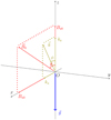 |
Fig. 1. Sketch of the configuration, with gravity along −z, and wavevector k, and magnetic field, B, in the x − z plane. |
where g is the magnitude of the gravitational acceleration g, assumed to be uniform. We use the temperature profile from the VALC model (Vernazza et al. 1981) and adopt the number density at the base of the atmosphere n0 = 2.84 × 10²¹ m−3. Figure 2 shows the equilibrium profiles of the temperature (left panel), density, and pressure (right panel). The magnetic field strength used in most simulations is B0 = 17.4 G, which makes the gas pressure equal to the magnetic pressure at the middle of our vertical domain, which extends from between 0.5 Mm and 2.1 Mm in height. The equipartition layer defined as the height where the sound speed equals the Alfvén speed is located higher than the height where the magnetic pressure equals the gas pressure, at ≈0.697 of the vertical domain. The equipartition layer separates the region of weak field regime at the bottom of the atmosphere from the region of strong field regime in the upper part of the atmosphere. When instead we use B0 = 52.3 G, the magnetic pressure equals the gas pressure at a height located at 1/4 of the vertical domain size.
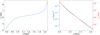 |
Fig. 2. Equilibrium temperature (left) and density pressure (right) as a function of height, z. |
In order to obtain a value for νA suitable for the VALC model atmosphere used in this work, we averaged the actual ηAρ2 in height from the full two-fluid model used in Popescu Braileanu et al. (2019), which gave a value of νA = 3.17 × 10⁻⁹ s kg m−3. The code MPI-AMRVAC2 (Keppens et al. 2021) uses nondimensional variables and the simulations presented in this work use a normalization for lengths equal to 106 m, for temperature measured in 5000 K and for number density 1020 m−3 and adopts magnetic units where the magnetic permeability is unity. In addition, we considered a plasma composed of Hydrogen only, and we used a ratio of specific heats γ = 5/3. This normalization gave a value of νA ≈ 10−4 in nondimensional units, which is used in all our simulations.
The value of the ambipolar coefficient in units of m2 s−1,  = ηA/μ0, calculated from the two-fluid model, composed by Hydrogen only, gravitationally stratified (Popescu Braileanu et al. 2019) and the value used in this work, for a magnetic field with strength B0 = 17.4 G, are shown for comparison in Fig. 3 (see also Fig. 5 from Khomenko et al. 2014). The ambipolar coefficient used in our simulations has a steeper increase with height, the difference being caused mainly by keeping a fixed ionization fraction in our case. We neglected other non-ideal effects such as Hall effect and Ohmic dissipation which have a larger contribution at the bottom of the atmosphere than the ambipolar effect (Fig. 5 Khomenko et al. 2014), because we wanted to distinguish the ambipolar effect. The ambipolar effect has a large contribution towards the upper boundary, where the collision frequency between ions and neutrals decreases.
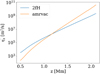 |
Fig. 3. Ambipolar coefficient in units of m2 s−1 as calculated from a two-fluid model (blue line) and the coefficient used in the simulations (orange line). |
2.3. Wave driving
The vertical domain between 0.5 Mm and 2.1 Mm is always covered by 3200 grid points. We generate a specific type of wave perturbation in the ghost cells at the bottom of our atmosphere, and this wave starts propagating in the unperturbed atmosphere described above. The horizontal domain varies with the type of wave perturbation that we study: it is between −0.5 Mm (megameter) and 0.5 Mm with 400 points for plane waves, between −1 Mm and 1 Mm with 600 points for the single Gaussian waves, and between −1.5 Mm and 1.5 Mm with 800 points for the two Gaussian wave simulations. The horizontal domain length is also specified in Table 1. We always use periodic boundary conditions in the x-direction and open boundary conditions for the perturbed quantities in the vertical direction for the upper boundary. The equations evolved by the code use a splitting of the density, pressure, and magnetic field variables into time-independent and time-dependent parts, where the time-independent variables correspond to the equilibrium variables ρ0, p0, and B0 that are mentioned above. In order to avoid reflection at the upper boundary, we used an absorbing layer of 0.1 Mm thickness at the top of our atmosphere. This layer is uniform, the gravity also being considered zero there. The time-dependent variables are damped exponentially in this layer:
 (9)
(9)
Simulations used in the paper.
where zdb = 2.1 Mm and zdt = 2.2 Mm are the bottom and the top of the layer respectively, and σd is a damping coefficient, constant for each simulation.
We used a three-step numerical scheme for the temporal integration and the HLL method for the calculation of the fluxes (Toro 1997) with a third-order slope limiter (Čada & Torrilhon 2009). As the ambipolar parabolic term imposes a very restrictive explicit CFL timestep, it has been implemented using the supertimestepping (STS) method, as described in the two variants available in the literature, one which uses Legendre polynomials, also known as RKL (Meyer et al. 2014; Xia & Keppens 2016; Xia et al. 2017; Stone et al. 2020), and the other which uses Chebyshev polynomials, also known as RKC (Alexiades et al. 1996; O’Sullivan & Downes 2006; O’Sullivan & Downes 2007; González-Morales et al. 2018; Nóbrega-Siverio et al. 2020). For the simulations presented in this work, we used the RKL method and a splitting technique of each temporal substep, which adds the ambipolar contribution before and after the contribution of the rest of the terms using half of the substep timestep. This splitting makes the temporal scheme accurate to the second order.
Our wave driver is based on an approximate analytical solution, as explained in the next section (Sect. 2.4). It involves (1) an amplitude for the imposed vertical velocity Vz = Ac0, where A is a free parameter and  is the (local) sound speed, (2) the period of the wave, and (3) the horizontal wave number kx. We then obtain the vertical wave number kz by solving a dispersion relation given by Eq. (A.2). From the four solutions, we choose the one corresponding to the fast upward wave. We will use two different shapes for the perturbation: a plane wave and a Gaussian wave, which uses a Gaussian function described by:
 (10)
(10)
We used σ = 8 km for all the simulations that have Gaussian perturbation and xc varied as shown in Table 1. There are five parameters which are varied in our simulations: the amplitude parameter A, the angle of the magnetic field with the vertical direction (θ), the strength of the initial uniform magnetic field B0, the period of the wave, and the local value of the angle ϕ between the propagation vector and the vertical direction at the base of the atmosphere. This angle ϕ is calculated from kx and kz, with kz obtained from the dispersion relation. The simulation parameters used in this paper are summarized in Table 1.
2.4. Approximate analytical solution
For the waves, we linearized the MHD equations given by Eq. (1) about the static equilibrium atmosphere. These linearized MHD equations, in terms of perturbations ρ1, p1, velocities vx, vy, and vz, and B1, for our 2D geometry with its uniform magnetic field, taking into account the ambipolar diffusivity, are as follows:
![Mathematical equation: $$ \begin{aligned}&\frac{\partial \rho _1}{\partial t} = - v_z \frac{\mathrm{d}\rho _0}{\mathrm{d}z} - \rho _0 \left[\frac{\partial v_x}{\partial x}+\frac{\partial v_z}{\partial z}\right],\nonumber \\&\rho _0 \frac{\partial v_x}{\partial t} = - \frac{\partial p_1}{\partial x} + B_{z0} J_{y1},\nonumber \\&\rho _0 \frac{\partial v_z}{\partial t} = -\rho _1 g - \frac{\partial p_1}{\partial z} - B_{x0} J_{y1},\nonumber \\&\frac{\partial p_1}{\partial t} = c_0^2 \frac{\partial \rho _1}{\partial t} + c_0^2 v_z \frac{\mathrm{d} \rho _0}{\mathrm{d} z} - v_z \frac{\mathrm{d} p_0}{\mathrm{d} z},\nonumber \\&\frac{\partial B_{x1}}{\partial t} = B_{z0}\frac{\partial v_x }{\partial z} - B_{x0}\frac{\partial v_z}{\partial z} + B_0^2 \left(\frac{\mathrm{d} \eta _{\rm A0}}{\mathrm{d} z}+\eta _{\rm A0} \frac{\partial }{\partial z}\right) J_{y1},\nonumber \\&\frac{\partial B_{z1}}{\partial t} = - B_{z0} \frac{\partial v_x}{\partial x} + B_{x0} \frac{\partial v_z}{\partial x}-B_0^2 \eta _{\rm A0} \frac{\partial }{\partial x} J_{y1}, \end{aligned} $$](/articles/aa/full_html/2021/09/aa40872-21/aa40872-21-eq13.gif) (11)
(11)
where we used the y-component of the perturbed current density
![Mathematical equation: $$ \begin{aligned} J_{y1}=\left[\frac{\partial B_{x1}}{\partial z}-\frac{\partial B_{z1}}{\partial x}\right]\cdot \end{aligned} $$](/articles/aa/full_html/2021/09/aa40872-21/aa40872-21-eq14.gif) (12)
(12)
We also used the fact that when ∂/∂y = 0, the linearized equations decouple completely, such that the only values that matter are the in-plane velocity perturbations, vx, vz, and magnetic perturbations Bx1 and Bz1. The equilibrium density profile also enters in  . We then introduce the ansatz where the dependence in time and in the x-direction of the perturbations are written explicitly as exp(iωt) and exp(−ikxx), respectively. The expressions for the vertical dependence of the perturbation in density and pressure are then obtained directly from the linearized continuity and pressure equations, when ω ≠ 0:
![Mathematical equation: $$ \begin{aligned}&\rho _1(z) = \frac{1}{\omega } \left[k_x \rho _0 v_x + i \left(\rho _0 \frac{\mathrm{d} v_z}{\mathrm{d} z}+ \frac{\mathrm{d} \rho _0}{\mathrm{d} z} v_z \right) \right],\nonumber \\&p_1(z) = \frac{1}{\omega } \left[k_x \rho _0 c_0^2 v_x + i \left(\rho _0 c_0^2 \frac{\mathrm{d} v_z}{\mathrm{d} z} - \rho _0 g v_z \right)\right]. \end{aligned} $$](/articles/aa/full_html/2021/09/aa40872-21/aa40872-21-eq16.gif) (13)
(13)
To make further analytic progress, we will first neglect the ambipolar effect, that is, we take ηA0 = 0. In that case, the linearized induction equation gives:
 (14)
(14)
After some manipulations, where we introduce the above expressions in the equations for x and z momentum, we obtain a system of two coupled ordinary differential equations (ODEs) for vx(z) and vz(z):
![Mathematical equation: $$ \begin{aligned}&\left(B_{x0}^2 + \gamma p_0\right) \frac{\mathrm{d}^2 v_z}{\mathrm{d} z^2}-\gamma \rho _0 g \frac{\mathrm{d} v_z}{\mathrm{d} z} + \left(\omega ^2 \rho _0 - k_x^2 B_{x0}^2 \right) v_z\nonumber \\&\qquad \qquad \qquad \qquad -B_{x0} B_{z0} \frac{\mathrm{d}^2 v_x}{\mathrm{d} z^2}- ik_x \gamma p_0 \frac{\mathrm{d} v_x}{\mathrm{d} z}\nonumber \\&\qquad \qquad \qquad \qquad +\left[k_x^2 B_{x0} B_{z0} - i k_x \rho _0 g(1-\gamma )\right] v_x = 0,\nonumber \\&B_{x0} B_{z0} \frac{\mathrm{d}^2 v_z}{\mathrm{d} z^2} + i k_x \gamma p_0 \frac{\mathrm{d} v_z}{\mathrm{d} z} - \left( k_x^2 B_{x0} B_{z0} + i k_x \rho _0 g \right) v_z\nonumber \\&\qquad \qquad \qquad \qquad -B_{z0}^2 \frac{\mathrm{d}^2 v_x}{\mathrm{d} z^2} - \left[\omega ^2 \rho _0- k_x^2 (B_{z0}^2 + \gamma p_0) \right] v_x = 0. \end{aligned} $$](/articles/aa/full_html/2021/09/aa40872-21/aa40872-21-eq18.gif) (15)
(15)
We can observe that when the field has no vertical component, Bz0 = 0, Eq. (15) reduce to a single second order ODE for the vertical velocity, equivalent to Eq. (5) from Nye & Thomas (1976). In the case where Bz0 = 0, it is also equivalent to Eq. (7.80) from Goedbloed et al. (2019), and that form shows the MHD continuous parts of the spectrum most clearly. In this special ky = 0 case, the Alfvén continuum drops out of the problem, and only leaves the slow continuum. The equations in Eq. (15) are equivalent to the coupled second order ODEs, as in Eqs. (2.9) and (2.10) from Cally (2006). The left-hand terms of the equations, as derived by Cally (2006), describe the acoustic and magnetic oscillations, and coupling terms describe the magnetic and the acoustic influence on these oscillations, respectively.
As our interest is in waves traveling through the atmosphere rather than solving the governing system of ODEs (which needs a sufficient amount of boundary conditions), we instead derive a local dispersion relation. We introduce in Eq. (15) a wave solution for the vertical direction, assuming that the vertical dependence of the perturbation is of the form exp(−ikzz). In this approximation, the perturbation of the magnetic field is locally perpendicular to the propagation direction at all heights,
 (16)
(16)
This local assumption gives us a relationship between the amplitude of the horizontal vx and vertical velocity, vz, and a local (i.e., with space-dependent coefficients) dispersion relation, which is a fourth-order equation in kz, for a given real frequency, ω, and wavenumber component, kx. The details of this Eq. (A.2) are given in Appendix A, where our approach is compared to previous treatments for waves in the magnetized, stratified atmosphere. The very same simple local dispersion analysis can also be carried out with a nonzero ambipolar coefficient, namely ηA ≠ 0. This case leads to more complicated expressions, where the calculations have been performed with the Mathematica software, but is just as in the ideal MHD case that leads to a fourth-order dispersion relation in kz similarly to Eq. (A.2).
We use the linear analysis from this local dispersion relation in our drivers as follows: for a given period (setting the given real ω) and horizontal wavenumber kx, we compute the (possibly complex) kz (and hence find ϕ from its real part, although we can also fix ϕ and compute kx, kz analogously) according to the local conditions (density, pressure, etc.) in the bottom ghost cells below our atmosphere. We then use the relations in Eqs. (13) and (14), as well as the relations between the velocity amplitudes from Eq. (A.1) in setting all perturbed quantities in accord with the selected wave solution. This involves taking the real part of the vz = Vzexp(iωt − ikxx − ikzz) prescription, and similarly for all other variables. For injected plane waves, this is adopted along the entire bottom boundary, whereas for Gaussian cases, this prescription is multiplied with a spatial Gaussian window function g, described in Eq. (10). As the ambipolar effect is negligible at the bottom of the atmosphere we use the same prescription for the driver in both MHD and ambipolar runs.
In order to have an analytical understanding of the simulations performed in this study we will use the dispersion relations (A.2) with the coefficients corresponding to the MHD and ambipolar situation. In our Appendix A, we compare our local dispersion relation approach to the Wentzel-Kramers-Brillouin (WKB) analysis obtained by Cally (2006) and to another approximate dispersion relation suggested by Thomas (1982). We find a very good agreement between the real parts of the complex wavenumbers kz, which determine the phase speeds of our fast and slow, upward and downward propagating waves. The imaginary parts, which relate to the damping of the waves as they propagate, are found to differ, but we go on to compare our nonlinear simulation results with our local predictions.
3. 2D simulation results
3.1. Ideal MHD preliminaries
3.1.1. Plane waves versus Gaussian pulse
Figure 4 shows snapshots of the vertical velocity for the simulations P-s, G-s, G-sr from Table 1. The waves driven for P-s and G-s have the same parameters, the only difference being in the type of perturbation, being a plane wave for P-s and a Gaussian for G-s. The horizontal mode number used for P-s and G-s is nx = 10, the horizontal wave number is calculated as kx = 2πnx/Lx, with the horizontal box length Lx given in Table 1, making the angle ϕ = 22.3°. For the G-sr wave we have nx = −10, reversing the orientation of the wavevector.
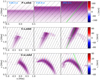 |
Fig. 4. Snapshots of vertical velocity for the plane wave P-s (top), the Gaussian pulse G-s (middle), and the reversed Gaussian G-sr (bottom) in the MHD case at three different moments. We note that the horizontal domain size differs for the three cases. |
When the upward traveling fast waves reach the equipartition layer, they usually split into two components, consisting of a fast wave that will become reflected and a slow mode that is transmitted higher up in the atmosphere. The transmission coefficient is shown to be (Schunker & Cally 2006b):
 (17)
(17)
where hs is equipartition layer scale height, which is the thickness of the layer over which vA0 ≈ c0, measured along the direction of propagation k. In Eq. (17), α is the angle between the direction of propagation of the wave and the magnetic field, so our notation gives this as α = |θ − ϕ|. The angle α for G-s and P-s corresponds to a wave which propagates almost parallel to the magnetic field. For this reason, the transmission from the fast to a slow wave is almost complete. This can be better seen in the snapshots for the Gaussian perturbation, G-s, where only a small fraction of the upward wave seems to be reflected at the height around 1.5 Mm. We note that the Gaussian wave is really a superposition of plane waves with wave numbers centered at the wave numbers corresponding to nx = 10, and different components reflect at slightly different heights, as can be observed in the snapshots for G-s (middle row of Fig. 4). Because of the larger corresponding angle α, the reversed Gaussian case G-sr is reflected. We can observe in Fig. 4 that the propagation speed and the reflection height of G-sr are similar to that of the reflected part of the G-s wave (bottom and middle rows).
Figure 5 shows the profile of the vertical velocity along the green line shown in the right panels of Fig. 4. We can observe that the plane wave case P-s and the Gaussian case G-s have similar profiles, with the only difference being a smaller amplitude for G-s because of the spreading suffered by the Gaussian pulse. The profile of the vertical velocity for the reversed Gaussian G-sr case is also similar to the profile of P-s and G-s in the bottom part of the atmosphere. This is because the bottom part corresponds to a weak field regime (vA0 ≪ c0) and the fast waves are then acoustic in nature, so they propagate with approximately the sound speed, regardless of the propagation angle and the magnetic field orientation. Higher up in the atmosphere, the propagation speed for G-sr becomes larger than for G-s (and P-s), and the amplitude of the vertical velocity drops, becoming negligible at the height z ≈ 1.5 Mm.
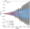 |
Fig. 5. Profile of vertical velocity along the green lines shown in Fig. 4, for the three cases shown there. |
3.1.2. Comparing the simulation with the local dispersion relation
The left panel of Fig. 6 shows the vertical velocity along the vertical line x = 0 for the plane wave case P-s. We use this vertical profile in order to obtain the real and imaginary part of the local “vertical wave number”, kz(z), corresponding to this wave. We use the positions of the maximum and minimum peaks, from which we determine the local wavelength and amplitude variation. Afterwards, we interpolate this data to obtain values in the whole vertical domain.
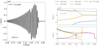 |
Fig. 6. Comparison between the numerical and analytical results for the simulations shown in Fig. 4. Left: profile of vertical velocity along x = 0 for P-s. Right: local dispersion relation corresponding to the simulations shown in Fig. 4. The complex vertical wavenumber kz(z) values calculated from the P-s simulation are overplotted on the dispersion diagram with the black dotted lines, up to the equipartition height, and they are clearly in perfect agreement with the upward fast wave (in green). |
The right panel of Fig. 6 shows the four solutions of the ideal MHD, local dispersion relation from Eq. (A.2) for this case. We overplotted the real and imaginary part obtained from the simulation P-s up to the equipartition height. We observe that there is a good match for both real and imaginary part between the simulation and the solution corresponding to the fast upward wave of our local dispersion relation (in Fig. 6, the green line for Solution 3). At the equipartition layer (at ≈1.25 Mm), there is a crossing of two solution branches, namely between the upward transmitted slow wave (red) and the fast wave (green). The fast wave is reflected above this point (at ≈1.5 Mm, we see the green line in Fig. 6 showing an infinite phase speed ω/Re(kz) and a pure damping). We observe that the reflection height at z = 1.5 Mm is consistent with its visual estimation from Fig. 4.
The upward solutions of the dispersion relation for the reversed Gaussian G-sr (nx = −10) could be also deduced from the dispersion diagram in the right panel of Fig. 6 for the nx = 10 case. Indeed, the upward slow and the fast wave corresponding to nx = −10 have for the real part a symmetric image in the positive domain and the same imaginary part as for Solutions 1 (in blue) and 2 (in orange) for nx = 10, respectively. In the dispersion diagram, we can visually see the transmission coefficient as the distance between the two solutions describing the fast and the slow waves at the equipartition layer. The fact that P-s and G-s are mostly transmitted compared to G-sr is then evident in the fact that curves that represent the real part of Solutions 3 and 4 are joined at z ≈ 1.25 Mm, compared to the larger distance seen between the curves at that position corresponding to Solutions 1 and 2. Thus, in order to compare G-sr to G-s (and P-s) from this diagram, we have to compare the orange line (by looking at the absolute value for the real part of kz) to the green line up to the equipartition height (z ≈ 1.25 Mm) and to the red curve above it. The larger propagation speed and smaller amplitude for G-sr compared to G-s (and P-s) above z ≈ 1 Mm can be deduced from this diagram.
3.2. Ideal MHD versus ambipolar cases
3.2.1. Varying the magnetic field inclination
Compared to the simulation P-s presented above, we then change the angle of propagation for the waves to a smaller inclination, ϕ = 10.9°. Next, we progressively change the angle of inclination of the magnetic field with the vertical direction from θ = 25.8° (plane wave P simulation), θ = 45° (Gaussian pulse G), and θ = 84.2° (plane wave case P-f). In this section, we compare the ideal MHD with cases where we also take into account the ambipolar effects.
Figures 7–9 show snapshots of P, G, and P-f simulations at different moments over time. The top and bottom panels show the MHD and ambipolar cases, respectively. The wave in the G case is mostly reflected. We can observe in all three cases that the wave amplitude is damped when the ambipolar diffusion is taken into account. For the G case, the ambipolar run shows therefore hardly any reflected wave. The interference patterns caused by interacting up and downward wave branches are clearly different between ideal MHD and ambipolar runs for P and P-f simulations. The effect of having a smaller inclination of the wave propagation with the vertical direction is an increase in the reflection height, which is now located at z ≈ 1.8 Mm.
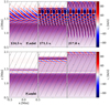 |
Fig. 7. Snapshots of vertical velocity for plane wave case P in the MHD case (top row) and ambipolar case (bottom row) at three different moments. We note the difference in interference patterns, which is almost absent for the ambipolar case. |
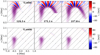 |
Fig. 8. Snapshots of vertical velocity for the Gaussian case G simulation in the MHD case (top row) and ambipolar case (bottom row) at three different moments. The reflected wave is almost absent in the ambipolar run. |
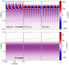 |
Fig. 9. Snapshots of vertical velocity for P-f simulation in the MHD case (top row) and ambipolar case (bottom row) at three different moments. We note the difference in the interference patterns, which is almost absent for the ambipolar case. |
The left and right panels of Fig. 10 show the profiles vz(z) of the vertical velocity at the vertical cut x = 0 for the plane wave P and P-f cases, respectively. The snapshots considered are taken before the waves reach the reflection point, so that we can easily distinguish between the upward and downward waves. In the left panel, the equipartition layer is marked by a vertical gray dotted line located at z = 1.3 Mm. We can observe the interference for the P case above the equipartition layer, which, at this moment, can only be explained by the fast and the slow waves propagating upwards. The transmission to the slow wave decreases in the P case, because α from the above Eq. (17) has increased, compared to the simulation P-s presented above. Therefore, the amplitude of the fast upward wave that will be reflected above the equipartition layer is larger than for the previous P-s case and the interference between the slow and the fast waves is clearly visible. In contrast, there is no visible interference for the case P-f and the wave seems to completely progress onto the fast branch. The interference patterns seen for P and P-f at later stages in Figs. 7 and 9 are related to the interaction between the upward fast wave driven from below, the downward reflected fast wave, and additionally the upward slow wave transmitted at the equipartition layer for the P case. The damping due to the ambipolar diffusion of the fast upward mode appears at earlier height and is larger for P-f compared to the P case.
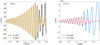 |
Fig. 10. Vertical cuts at x = 0 for the vertical velocity, for both the MHD and the ambipolar runs from Figs. 7–9. Left: plane wave case P. The vertical dot-dashed gray line located at the height z = 1.3 Mm marks the equipartition layer. Right: fast plane wave case P-f. |
3.2.2. Analysis using the local dispersion relation
We observe from the left panel of Fig. 11, which shows the real part of the relevant dispersion relation solutions, that the three waves (P, G, and P-f) are subject to a reflection at the same point, namely at ≈1.85 Mm, which is where Re(kz) vanishes, namely, higher up in the atmosphere than in the previous case of P-s. The reflection height, marked by a vertical black dotted line at z = 1.85 Mm that is deduced from this diagram is consistent with that observed in Fig. 8. We can also observe that the transmission coefficient is smaller for larger θ (also larger α for these cases as ϕ was kept constant), which is seen as the gap width between solutions widens at the equipartition layer (marked in the panel by a dot-dashed gray line at z = 1.3 Mm). This is consistent with the result obtained by Cally (2006) and with the comparison of the previous simulations, G-s and G-sr.
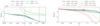 |
Fig. 11. Comparison of the analytical results when the angle between the magnetic field and the direction of propagation is varied, corresponding to the cases shown in Figs. 7–9. Left: solutions 3 and 4 for the real part of the vertical wavenumber kz corresponding to the cases P (θ = 25.8°), and G (θ = 45°), as well as Solution 3 for case P-f (θ = 84.2°). The vertical dot-dashed gray line at z = 1.3 Mm, which is also present in left panel of Fig. 10, marks the equipartition layer. The vertical dotted black line at z = 1.85 Mm shows the reflection height. Right: solution 3 for the imaginary part of the vertical wavenumber kz corresponding to the three cases P (θ = 25.8°), G (θ = 45°) and P-f (θ = 84.2°), for both MHD and ambipolar cases. The points where the imaginary part diverges in the ambipolar case compared to the MHD case are indicated with markers in the panel. |
The right panel of Fig. 11 shows that for larger θ the damping of the amplitude of the vertical velocity appears earlier in the atmosphere for larger θ for the fast wave solution (Solution 3). This is consistent with the results obtained from the simulations, as shown in Fig. 10. The ambipolar diffusion introduces a contribution to the electric field through a drift velocity that is proportional to the Lorentz force. Thus, in the case of the fast waves, the velocity drift is proportional to the magnetic pressure gradient, which is larger for propagation running perpendicular to the field lines.
3.3. Varying the wave parameters
In order to observe the slow wave, we increased the angle of propagation at the bottom of the atmosphere to ϕ = 49.5°, compared to the P case, so that the fast component reflects at a lower height. As the vertical wave number decreases, the solutions of the local dispersion relation give a worse approximation. We only show in Fig. 12 the profile of the vertical velocity at x = 0, in the simulations P-a (left panel) and P-as (right panel), for both MHD and ambipolar runs. The angle of inclination of the background magnetic field with the vertical direction for P-a is the same as in the simulation P, θ = 25.8°. For the P-as simulation, the angle θ is increased – with this being the only difference to the P-a case. For the P-as case, θ = ϕ, enhancing the transmission of the slow wave.
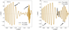 |
Fig. 12. Vertical cut at x = 0 for the vertical velocity for plane wave case P-a (left panel) and P-as (right panel). The upward fast (FU) and the slow (S) components are indicated in both panels. We compare MHD (black solid lines) with the ambipolar (orange dashed lines) case. |
In both cases, in the lower part of the domain, we can observe the fast upward wave driven at the bottom, before it interferes with the reflected fast component. The slow wave can now be clearly seen as a wave packet after the reflection height of the fast wave. We can observe that the fraction of the reflected component in the case P-as is larger than for the case P-s (see Fig. 5, where there is no visible interference because the wave is almost completely transmitted), where the direction of propagation at the base had also the same angle (ϕ) as the background magnetic field (θ) with the vertical direction. The possible cause is the increase in the angle ϕ.
We observe in Fig. 12 that the fast components for both P-a and P-as are subject to reflection before the ambipolar term has any effect. We can observe this by comparing the two panels to see that the reflection height for P-a is larger than for P-as. The damping of the slow wave in the ambipolar case is more pronounced at a lower height.
We then increase the plane wave period to P = 20 s. We consider the same angle ϕ = 49.5° and two values of θ, namely θ = 22.5° (simulation P-p) and θ = 84.2° (simulation P-pf). The only difference between the simulations P-p and P-a presented above is a larger period for the P-p case.
By using a local dispersion relation, Bel & Leroy (1977), for waves that propagate in the vertical direction in an isothermal atmosphere, found that there is a cutoff period which increases with the density scale height. That means that waves with periods larger than the cutoff period do not propagate. Their result was obtained for the slow modes in the general case, and for the fast modes in the case of horizontal magnetic field. For the slow modes, the cutoff period also increases with the inclination of the direction of the magnetic field. In our case, as our temperature varies with height, this result applied locally means that waves with larger periods are reflected at smaller heights in the atmosphere.
The left and right panel of Fig. 13 show a vertical cut at x = 0 for the vertical velocity for the 20 s period cases P-p and P-pf, respectively. We can observe from the left panel of Fig. 13 that the fast wave for P-p reflects at a smaller height compared to P-a, which might be due to a larger period for the P-p case, this being the only difference between the two cases.
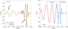 |
Fig. 13. Vertical cut at x = 0 for the vertical velocity, for both MHD and ambipolar cases. Left: case P-p, upward fast (FU) and slow (S) components. Right: P-pf. |
From the right panel we can observe that the reflection height is increased for larger θ. This fact has been also observed for the case P-a compared to P-as, which is presented above.
The fast component in the P-p case is reflected before the ambipolar term has any effect. However, as the wave P-pf reflects at higher height we can observe the ambipolar effect on the fast component above z ≈ 1.25 Mm for the P-pf case. The ambipolar effect on the fast component seems to be smaller than for smaller periods, if we compare P-pf to P and G cases which have smaller α than P-pf. The slow component has a larger amplitude than the fast component and is slightly more damped by the ambipolar diffusion for the P-p case compared to the P-a case.
3.4. Varying the magnetic field strength
Figure 14 shows the vertical velocity profile along x = 0 for the simulation P-b at two moments in time. All the parameters of the simulation P-b are the same as for the simulation P (from the left panel in Fig. 10), with the difference that the magnetic field is increased. For this reason, the equipartition layer is now located at a lower height (≈0.85 Mm) compared to the P case.
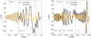 |
Fig. 14. Vertical cuts at x = 0 for the vertical velocity for the simulation P-b at two different times (note the changing axis scales). This can be compared with the weaker field strength case from Fig. 10, left panel. The equipartition height is shown by a vertical light blue dotted line located at z = 0.85 Mm in both panels. Right panel: the vertical dotted dark blue line located at z = 1.42 Mm indicates the reflection height of the fast component. The wave modes: upward fast (FU), slow (S), and downward fast (FD) present in each of the regions are indicated in the panels. |
The panel at the left hand side shows a snapshot taken before the fast wave reached the reflection height. We can observe a similar interference between the fast and the slow wave as in the P simulation, with the difference that it starts at a smaller height. We can also observe that the fast wave starts to be damped by the ambipolar diffusion earlier in the atmosphere, so that the fast mode is more affected by the ambipolar diffusion in the P-b case as compared to the P case (see left panel of Fig. 10).
The panel at the right hand side shows a snapshot taken before the wave reaches the upper boundary, so that we can observe the slow transmitted wave. The effect of the ambipolar diffusion on the slow wave seems to be larger for P-b compared to P-a (see left panel of Fig. 12), which can be attributed to a larger magnetic field, the angle α being larger in the P-a case as compared to the P-b case. The damping of the slow mode decreases towards the upper part of the atmosphere, similarly to the cases of P-a and P-as.
Figure 15 compares the solutions of the dispersion relations for the case P and P-b. Left panel shows the real part of Solutions 3 and 4, the upward fast and slow modes, respectively, for the MHD case for the two cases: P (black and gray solid lines) and P-b (dark and light blue solid lines), as indicated in the legend. The equipartition layer is indicated by vertical dot-dashed gray and light blue lines for P and P-b, respectively. The reflection height of the fast component is indicated by a vertical dotted black line for P and a vertical dotted dark blue for P-b.
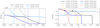 |
Fig. 15. Relevant solutions (3 and 4) of the local dispersion relation for the real (left) and imaginary (right) part of the vertical wavenumber kz corresponding to the cases P (B0 = 17.4G) and P-b (B0 = 52.3). The MHD solutions are indicated by solid lines in both panels. Left panel: the reflection heights for the fast component are indicated by black and blue vertical dotted lines for P and P-b, respectively. The equipartition heights are shown with a gray and light blue vertical dot-dashed lines for P and P-b, respectively. Right panel: we also show Solutions 3 and 4 for the ambipolar cases with dashed lines. The points where the ambipolar and MHD Solution 3 (fast modes) diverge are indicated by the markers for both P (black marker) and P-b (blue marker) cases. |
The right panel of Fig. 15 shows the imaginary part of Solutions 3 and 4, for the MHD case for the two cases: P and P-b, keeping the same color coding. Additionally, we show the imaginary part of these solutions in the ambipolar case with dashed lines, as indicated in the legend. The points where the imaginary part of Solution 3 in the MHD case diverges from the ambipolar case are indicated by a black and blue marker in the P and P-b case, respectively. Above this diverging height, the ambipolar effects produce a damping of the fast wave components compared to MHD cases. We can observe all three of the following shifted to an earlier height in the P-b case compared to P: (1) the equipartition layer, (2) the diverging height, and (3) the reflection height.
The slow modes are also more affected when the magnetic field is increased. This can be seen in the diagram as the area between Solution 4 for the ambipolar and MHD cases above the equipartition layer, which is clearly larger for P-b (area between pink dashed line and light blue solid line above z ≈ 0.8 Mm), compared to the P case (area between yellow dashed and gray solid lines above z ≈ 1.25 Mm). However, the damping decreases in the upper part of the domain, where it seems that the ambipolar effects produce no damping of the slow modes. This can be visually seen in the overlapping of the pink dashed line to the light blue solid line in the P-b case, and the yellow dashed to the gray solid line in the P case. These estimations are consistent with the results of the simulations.
4. More complex setups: Interacting pulses
We next consider a more complex case, in which the perturbation used for simulation 2G is a superposition of the perturbations used in G-s and G-sr, where the centers of the two Gaussians are separated by 1.2 Mm. Hence, this 2G simulation involves two Gaussians that will necessarily interact. The amplitude of the waves is also increased by a factor of 100, compared to the previous simulations, so that nonlinear effects become more important. The interaction of the two waves creates small scales, an effect amplified by the fact that we used larger amplitudes for this simulation. Figure 16 shows snapshots of vertical velocity for the 2G simulation taken at different moments in time, and this for both the MHD and the ambipolar case. A small fraction of the left Gaussian waves effect a reflection at z ≈ 1.5 Mm, above the equipartition layer at the same height as the waves from the right Gaussian pulse. The right Gaussian pulse is driven at the bottom of the atmosphere at a higher angle with respect to the magnetic field, and undergoes an almost complete reflection. The behavior of the individual left and right Gaussian pulses in the linear regime can be observed in Fig. 5, in the snapshots of G-s and G-sr, respectively.
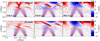 |
Fig. 16. Snapshots of the vertical velocity for the simulation 2G, the MHD case (upper panels) and ambipolar case (bottom panels) taken at three moments in time. |
The fast driver wave is acoustic in nature in the deep layers where the magnetic field is weak, and the wave propagates isotropically. The gravity as a restoring force is less important than the gas pressure gradient, and the velocity oscillates along the direction of the propagation mainly. Higher up in the atmosphere, above the equipartition layer located at z ≈ 1.25 Mm, when the field becomes strong, the fast wave becomes magnetic in nature, and it propagates mainly across the field lines. The slow wave there becomes acoustic in nature, and it propagates mostly along the field lines. The dominant restoring force is the gradient of the gas pressure and the velocity oscillates mainly along the direction of propagation, parallel to the field lines. The perturbation of the magnetic field is small for the slow modes.
Above the equipartition layer, where the dynamics is dominated by the magnetic field, the fast and the slow wave can be highlighted by looking at the components of the velocity along and perpendicular to the magnetic field. Figure 17 shows the components of the velocity perpendicular (left panels) and parallel (right panels) to the magnetic field, with the same colormap and normalization as for Fig. 16, for an easier comparison. The top panels display the MHD case, and the bottom panels display the case when the ambipolar diffusion is present. The horizontal black dotted lines located at z = 1.5 Mm represent the reflection height of the fast upward wave for the central component of the Gaussian waves, which is a superposition of plane waves. Additionally, the equipartition layer is shown in the right panels by the gray dotted line at z = 1.25 Mm. Below the reflection height (black dotted line), the fast upward and downward components can be seen in both left and right panel.
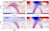 |
Fig. 17. Snapshots of the components of velocity perpendicular (left panels) and parallel (right panels) to the magnetic field for simulation 2G, for the MHD case (upper panels) and ambipolar case (bottom panels), taken at 198.1 s. This can be compared with the rightmost panels in Fig. 16, where we showed vz at the same time. The horizontal gray and black dotted lines present in the panels at the right hand side located at the heights z = 1.25 Mm and z = 1.5 Mm represent the equipartition layer and the reflection height, respectively. Above the reflection height the only wave which propagates is the slow mode, with the velocity oscillating along the magnetic field lines, observed in the right panel. |
Above the equipartition layer, the fast upward waves change the direction of propagation to being perpendicular to the magnetic field lines, and this is better seen in the left panels. Above the equipartition layer, the fast upward waves split into a fast component which reflects higher up (at the height about the black dotted line) and the slow component. The velocity of the slow component oscillates mainly along the field lines, so the slow component appears in the right panels. Above the reflection height, only the slow component is present, seen in the right panels. The fact that we still see fast components a bit above the reflection height is related to the same argument mentioned before for the Gaussian perturbations, namely that different modes present in the superposition reflect at slightly different height. The ambipolar effect, which starts to be important at about the equipartition layer, cannot be visually observed below this height. Above the equipartition point, we can visually observe less damping in the ambipolar case in the right panel associated to the slow wave.
5. Analysis of wave heating
When the ambipolar diffusivity is present, the wave does indeed work against the Lorentz force, and loses kinetic energy to magnetic energy. The loss of the kinetic energy is seen in the damping of the wave in the ambipolar case. The ambipolar diffusion converts the magnetic energy into heat through the dissipation of the electric field, resulting in an increase in temperature. The mean magnetic energy is smaller when the ambipolar diffusion is considered, compared to pure MHD cases.
The increase in the temperature of the atmosphere depends on the total energy present in the domain, which is different for the various cases we showed, so it is difficult to compare between cases. Energy is introduced at a constant rate by driving the wave through the bottom boundary, which also depends on the parameters of the wave (amplitude, wavevector, period). At the open upper boundary, energy might escape or even enter the domain, and this variation in energy can depend on time. These effects are supposedly similar for MHD versus ambipolar runs, so we will rather intercompare identical cases.
The left panel of Fig. 18 shows the difference in the average temperature for several simulations in the MHD and ambipolar cases. The right panel of Fig. 18 shows spatial average of the ambipolar heating term, as a source term in the temperature equation,
 (18)
(18)
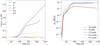 |
Fig. 18. Time evolution of the average of the difference in the mean temperature between the ambipolar and MHD simulations (left panel) and the increase in temperature in a unit of time corresponding to the ambipolar heating ha (right panel). The averages are done in the z-direction between the heights 0.8 and 1.7 Mm, and in the x-direction. To ease the comparison, the quantities have been normalized using the value r, defined in Eq. (19). |
The spatial average has been done in the horizontal direction and in the vertical direction between heights of z = 0.8 and z = 1.7 Mm. For an easier comparison between the 2G case, which used a larger amplitude and a different shape of the perturbation, with the rest of the cases, the values have been multiplied by a normalization constant:
 (19)
(19)
where l is the fraction of the domain where the perturbation is applied, that is, for the 2G case:
![Mathematical equation: $$ \begin{aligned} l=&\frac{1}{3}\int _{-1.5}^{1.5}\left[{\exp }\left(-\frac{(z-0.6)^2}{2 (0.08)^2}\right)\right.\nonumber \\&+{\exp }\left.\left(-\frac{(z+0.6)^2}{2 (0.08)^2}\right)\right]\mathrm{d}z, \end{aligned} $$](/articles/aa/full_html/2021/09/aa40872-21/aa40872-21-eq23.gif) (20)
(20)
and a is the amplitude ratio, having a = 100 for the 2G case. This gives the value of r = 5.625 × 10⁻³ for the 2G case, and r = 1 for all the other cases shown in Fig. 18.
For all the simulations, except for the strongly nonlinear 2G case, the increase in temperature is larger in the ambipolar case when compared to its MHD equivalent. The conversion to heat is more efficient through compression than through the ambipolar heating in this case.
The ambipolar heating term increases in time while the wave propagates towards the top of the domain, when it becomes flat. At later times, the formation of small scale structures enhances the ambipolar diffusion. The small scales are formed by the nonlinear interaction of the two Gaussian pulses in the 2G case, or by the interaction of the upwards going waves and the reflected fast downward waves for P, P-f, and P-b cases. In the P and P-b cases there are two waves propagating upwards above the equipartition layer, the slow and the fast modes, while for P-f only the fast mode exists. For this reason, the ambipolar heating for the simulation P becomes similar to P-f simulation during late evolution, even if the latter has more magnetic energy. In order to understand the distribution of the magnetic energy, we go on calculate the Fourier spectra in both simulations, P and P-f, for the MHD and ambipolar case.
Figure 19 shows the Fourier amplitudes of the magnetic energy perturbation (obtained using a fast Fourier transform in the x-direction) averaged in height between z = 0.8 Mm and z = 1.7 Mm as a function of the horizontal mode number for the same time in the P (left panel) and P-f (right panel) simulations. We show the spectra for both the MHD (blue lines) and ambipolar (red lines) cases. We can observe that the mean magnetic energy perturbation (the amplitude of mode n = 0, shown in the legend) is larger for the P-f simulation, compared to the P simulation for both MHD and ambipolar cases. In the MHD case, the amplitudes of the modes with numbers which are multiples of the number of the driven mode (n = 5) are slightly larger for P-f compared to P, however, intermediate scales (with mode numbers not multiples of 5), have more magnetic energy in P simulation compared to P-f. The magnetic energy dissipated by ambipolar effect, which can be seen as the difference between the blue and the red curves, seems to be larger for most of the scales in the P case, especially for the smaller ones. We conclude that the existence of the additional slow transmitted mode in the P simulation, besides the fast upward and fast downward (reflected) modes present in both simulations, enhances the ambipolar diffusion as a consequence of the formation of small scale structures through the (nonlinear) interaction of these waves.
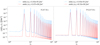 |
Fig. 19. Fourier amplitudes of the magnetic energy perturbation for the MHD simulations and the simulations with ambipolar effect included as a function of the horizontal mode number for the cases: P (left) and P-f (right). The amplitudes are calculated by a FFT transform in the x-direction for a snapshot taken at time t = 217.8 s and averaged in height between 0.8 Mm and 1.7 Mm. |
6. Conclusions
In this work, we perform simulations of waves to examine the ambipolar effect in the single fluid MHD model. Dispersion diagrams obtained from approximate analytical solutions to the linearized governing equations helped us to understand the results of the simulations. We varied parameters related to the background atmosphere and related to the properties of the waves, and we studied how this impacts the effects of the ambipolar diffusion. The main conclusion is that ambipolar diffusion does not affect the wave propagation, but, rather, the wave amplitude, effectively damping the wave. This finding is similar to the conclusion reached by Cally & Khomenko (2018). However, in our study we make a detailed analysis of the different parameters that can influence the results, with a clear separation between the effects on fast and slow modes. As a secondary effect, wave interference structures formed from the interaction of different types of waves are shown and seen to be affected by ambipolar diffusion in different ways. The main effects of the ambipolar diffusion are summarized below.
-
Fast waves are more affected by ambipolar diffusion when their propagation is perpendicular to the magnetic field. A larger angle of propagation between the direction of propagation at the base of the atmosphere and the magnetic field makes the ambipolar damping effect larger also for the slow modes.
-
Ambipolar diffusion affects the waves with smaller periods to a greater extent, with regard to fast modes. Fast waves with a large angle of propagation with respect to the vertical direction, or large periods, undergo reflection before being affected by ambipolar diffusion. A larger inclination of the magnetic field with the vertical direction will allow fast components of waves with larger period to propagate higher up in the atmosphere where they can be damped by ambipolar diffusion.
-
The damping due to ambipolar diffusion is larger for larger magnetic field. For the fast wave, this is especially relevant because the ambipolar damping starts earlier in the atmosphere. The slow modes are also more damped for larger magnetic fields.
-
Slow waves are less affected by the ambipolar diffusion, compared to fast modes at the same height. The damping of the slow waves decreases at larger heights.
-
The mean temperature is generally larger for the simulations with ambipolar diffusion, compared to the MHD simulations. However, compressive heating could prove more efficient than the ambipolar heating.
-
Small-scale gradients enhance the ambipolar diffusion. In our simulations, the small scales are created by nonlinear effects, which are more pronounced for larger amplitudes of the driven waves or by the (nonlinear) interaction of different modes.
Acknowledgments
This work was supported by the ERC Advanced Grant PROMINENT and a joint FWO-NSFC grant G0E9619N. This project has received funding from the European Research Council (ERC) under the European Union’s Horizon 2020 research and innovation programme (grant agreement No. 833251 PROMINENT ERC-ADG 2018). This research is further supported by Internal funds KU Leuven, through a PDM mandate and the project C14/19/089 TRACESpace.
References
- Alexiades, V., Amiez, G., & Gremaud, P.-A. 1996, Commun. Numer. Meth. Eng., 12, 31 [Google Scholar]
- Bai, X.-N., & Stone, J. M. 2011, ApJ, 736, 144 [NASA ADS] [CrossRef] [Google Scholar]
- Bel, N., & Leroy, B. 1977, A&A, 55, 239 [NASA ADS] [Google Scholar]
- Brandenburg, A. 2019, MNRAS, 487, 2673 [NASA ADS] [CrossRef] [Google Scholar]
- Čada, M., & Torrilhon, M. 2009, J. Comput. Phys., 228, 4118 [NASA ADS] [CrossRef] [Google Scholar]
- Cally, P. S. 2001, ApJ, 548, 473 [Google Scholar]
- Cally, P. S. 2005, MNRAS, 358, 353 [Google Scholar]
- Cally, P. S. 2006, Philos. Trans.: Math. Phys. Eng. Sci., 364, 333 [NASA ADS] [Google Scholar]
- Cally, P. S., & Khomenko, E. 2018, ApJ, 856, 20 [NASA ADS] [CrossRef] [Google Scholar]
- Goedbloed, H., Keppens, R., & Poedts, S. 2019, Magnetohydrodynamics of Laboratory and Astrophysical Plasmas (Cambridge: Cambridge University Press) [Google Scholar]
- González-Morales, P. A., Khomenko, E., Downes, T. P., & de Vicente, A. 2018, A&A, 615, A67 [NASA ADS] [CrossRef] [EDP Sciences] [Google Scholar]
- Hoyos, J. H., Reisenegger, A., & Valdivia, J. A. 2010, MNRAS, 408, 1730 [CrossRef] [Google Scholar]
- Jones, P. B. 1987, MNRAS, 228, 513 [NASA ADS] [CrossRef] [Google Scholar]
- Keppens, R., Teunissen, J., Xia, C., & Porth, O. 2021, Comput. Math. Appl., 81, 316 [Google Scholar]
- Khomenko, E. 2009, in Solar-Stellar Dynamos as Revealed by Helio- and Asteroseismology: GONG 2008/SOHO 21, eds. M. Dikpati, T. Arentoft, I. González Hernández, C. Lindsey, & F. Hill, ASP Conf. Ser., 416, 31 [NASA ADS] [Google Scholar]
- Khomenko, E., Collados, M., Díaz, A., & Vitas, N. 2014, Phys. Plasmas, 21, 092901 [NASA ADS] [CrossRef] [Google Scholar]
- Meyer, C. D., Balsara, D. S., & Aslam, T. D. 2014, J. Comput. Phys., 257, 594 [NASA ADS] [CrossRef] [Google Scholar]
- Musielak, Z. E., Rosner, R., Stein, R. F., & Ulmschneider, P. 1994, ApJ, 423, 474 [Google Scholar]
- Nóbrega-Siverio, D., Martínez-Sykora, J., Moreno-Insertis, F., & Carlsson, M. 2020, A&A, 638, A79 [EDP Sciences] [Google Scholar]
- Nye, A. H., & Thomas, J. H. 1976, ApJ, 204, 573 [NASA ADS] [CrossRef] [Google Scholar]
- O’Sullivan, S., & Downes, T. P. 2006, MNRAS, 366, 1329 [NASA ADS] [CrossRef] [Google Scholar]
- O’Sullivan, S., & Downes, T. P. 2007, MNRAS, 376, 1648 [NASA ADS] [CrossRef] [Google Scholar]
- Popescu Braileanu, B. 2020, PhD Thesis, University of La Laguna, Spain [Google Scholar]
- Popescu Braileanu, B., Lukin, V. S., Khomenko, E., & de Vicente, Á. 2019, A&A, 630, A79 [NASA ADS] [CrossRef] [EDP Sciences] [Google Scholar]
- Schunker, H., & Cally, P. 2006a, in Proceedings of SOHO 18/GONG 2006/HELAS I, Beyond the Spherical Sun, eds. K. Fletcher, & M. Thompson, ESA Spec. Publ., 624, 5 [NASA ADS] [Google Scholar]
- Schunker, H., & Cally, P. S. 2006b, MNRAS, 372, 551 [Google Scholar]
- Sinha, M. 2020, ArXiv e-prints [arXiv:2010.10776] [Google Scholar]
- Spruit, H. C., & Bogdan, T. J. 1992, ApJ, 391, L109 [Google Scholar]
- Stone, J. M., Tomida, K., White, C. J., & Felker, K. G. 2020, ApJS, 249, 4 [Google Scholar]
- Thomas, J. H. 1982, ApJ, 262, 760 [Google Scholar]
- Thomas, J. H. 1983, Annu. Rev. Fluid Mech., 15, 321 [Google Scholar]
- Toro, E. F. 1997, The HLL and HLLC Riemann Solvers (Berlin, Heidelberg: Springer-Verlag), 293 [Google Scholar]
- Vernazza, J. E., Avrett, E. H., & Loeser, R. 1981, ApJS, 45, 635 [Google Scholar]
- Xia, C., & Keppens, R. 2016, ApJ, 823, 22 [Google Scholar]
- Xia, C., Keppens, R., & Fang, X. 2017, A&A, 603, A42 [NASA ADS] [CrossRef] [EDP Sciences] [Google Scholar]
- Zhugzhda, I. D., & Dzhalilov, N. S. 1984, A&A, 132, 45 [NASA ADS] [Google Scholar]
Appendix A: Comparing local dispersion relations for MHD
For the gravito-magneto-acoustic waves described by two coupled second-order ODEs, Eq. (15) offer an exact analytical solution for an isothermal atmosphere in terms of Meijer (Zhugzhda & Dzhalilov 1984) or hypergeometric (Cally 2001) functions. However, this solution is not possible when the ambipolar diffusion is considered; moreover, a local dispersion relation gives more intuitive insight about the behavior of the waves.
The assumption of a Fourier variation exp(−ikzz) in Eq. (15) ignores the fact that the vertical direction is not uniform, but does lead to a local dispersion relation. In doing so, we obtain a relationship between the amplitudes Vx, Vz of the horizontal vx and vertical velocity vz perturbation, given by:
 (A.1)
(A.1)
along with a space dependent local dispersion relation, which is a fourth-order equation in kz, for a given real ω and kx, hence of the form:
 (A.2)
(A.2)
where the coefficients are,
![Mathematical equation: $$ \begin{aligned}&a_4 = B_{z0}^2 c_0^2 \rho _0,\nonumber \\&a_3 = B_{z0} \left[2k_x B_{x0} \gamma p_0- i B_{z0} \gamma \rho _0 g\right],\nonumber \\&a_2 = k_x^2 B_0^2 \gamma p_0 -i k_x B_{x0} B_{z0} \gamma \rho _0 g-\omega ^2 \rho _0 (B_0^2+\gamma p_0),\nonumber \\&a_1 = 2k_x^3 B_{x0} B_{z0} \gamma p_0+i(\omega ^2\rho _0-k_x^2 B_{z0}^2)\gamma \rho _0 g,\nonumber \\&a_0 = k_x^4 B_{x0}^2\gamma p_0 -i k_x^3B_{x0} B_{z0} \gamma \rho _0 g \nonumber \\&\qquad -k_x^2\left[\rho _0^2g^2(1-\gamma )+\omega ^2\rho _0(B_0^2+\gamma p_0)\right]+\omega ^4\rho _0^2. \end{aligned} $$](/articles/aa/full_html/2021/09/aa40872-21/aa40872-21-eq26.gif) (A.3)
(A.3)
The formal infinities which appear in the atmosphere when D = 0 in the above Eq. (A.1) do not concern us here, since our bottom driver avoids having this situation.
The WKB method applied by Cally (2006) consists in first making a linear transformation of the variables so that the operator applied to the amplitudes of the new variables is self-adjoint. This means that at zeroth order, the amplitudes of the new variables are constant and from a physical point of view, this is related to the conservation of energy in a stratified atmosphere. The combination used by Cally (2006) is given by:
 (A.4)
(A.4)
where ξ = (ξx, 0, ξz) is the displacement variable, a0 is the Alfvén speed, and θ is the angle of the magnetic field with the vertical direction. This ξ is related to the velocity through v = iωξ. The dispersion relation obtained is Eq. (2.12) from Cally (2006):
![Mathematical equation: $$ \begin{aligned}&(1-\varepsilon ^4) \omega ^4 - \left[a_0^2 + (1-\varepsilon ^4)c_0^2 \right] k^2 \omega ^2 +(1-\varepsilon ^4) a_0^2 c_0^2 k^2 k_\parallel ^2 \nonumber \\&\qquad \qquad -\left[(1-\varepsilon ^4) \omega ^2 - a_0^2 k^2\right] \left[\omega _{\rm c}^2 - (c_0^2 N^2 k_x^2)/\omega ^2 \right] \nonumber \\&\qquad \qquad -a_0^2 k^2 \omega _{\mathrm{c}i}^2 \left[{\sin }^2\theta + \varepsilon ^4 {\cos }^2\theta \right] + \frac{a_0^2 c_0^2 k^2 k_x \varepsilon ^2}{H}=0, \end{aligned} $$](/articles/aa/full_html/2021/09/aa40872-21/aa40872-21-eq28.gif) (A.5)
(A.5)
where:
 (A.6)
(A.6)
When dissipation mechanisms are considered, the WKB method, as described by Cally (2006) cannot be applied as no self-adjoint operator can be found. In these cases, and even in cases with no dissipation, when finding the right linear combination of variables was not straightforward, the wave solution in the vertical direction was directly introduced in the linearized equations and local dispersion relations were obtained at the zeroth order which neglects the vertical variations of the amplitudes. The validity of the local dispersion relation is restricted to the range |kz|H ≫ 1, where H is the density gradient scale length (Thomas 1983). The local dispersion relation is not unique and generally depends on the sequence of steps in the derivation (Thomas 1982). Thomas (1982, 1983) suggested that all the terms of order one or higher in kzH−1 should be neglected in order to obtain a unique unambiguous form for the dispersion relation, further mentioned as approximate dispersion relation. If, instead, we introduce the wave solution for the vertical direction directly in Eq. (11), we would obtain a slightly different dispersion relation than that described by Eq. (A.2), where in this case with uniform magnetic field, the difference comes only from the term ∂p1/∂z, which introduces terms related to equilibrium derivatives. For the same reason, changing variables to linear combinations of them which involve equilibrium profiles, changes slightly the dispersion relation obtained. The dispersion relation obtained for an isothermal atmosphere, by directly introducing the vertical wave solution in the linearized equations is given by Eq. (3.6) from Thomas (1983), which for the 2D case is:
 (A.7)
(A.7)
Figure A.1 compares the four solutions of the three dispersion relations obtained in the MHD approximation: the dispersion relation used by Cally (2006) in the WKB approach, Eq. (A.5) (labeled “s.a.”), the approximate dispersion relation obtained by Thomas (1983), i.e. Eq. (A.7) (labeled “appr.”) and the local dispersion relation used in this work, Eq. (A.2) (labeled “local”). The dispersion relation has been solved for each height using the local parameters of the background atmosphere, corresponding to the simulation P. The right panels correspond to a zoom indicated on the right axis of the left panels. The downward propagating solutions have been obtained by reversing the horizontal wave number, indicated by the labels “nx = 5” and “nx = −5”. In this way, we can test that the upward and downward solutions for the real part are symmetric. The real part is related to wave propagation, Solutions 1 and 4 correspond to the slow waves which propagate downwards and upwards respectively and Solutions 2 and 3 correspond to downward and upward fast waves. The imaginary part is related to the amplification or damping of the amplitude, for the waves propagating upwards a positive value being related to amplification and a negative value to damping, and the reverse for the downward waves.
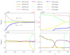 |
Fig. A.1. Case P: four solutions of the dispersion relation for the MHD case in the three approximations: local dispersion relation, self-adjoint operator, approximate dispersion relation. Right panels: zoom in the left panels for the limits shown as red ticks on the right axis of the left panels. |
We can observe that the three approximations give similar symmetric solutions for the real part. The imaginary part of the solutions are however different in the three approximations. The dispersion relation obtained from a self-adjoint operator, “s.a.” has the imaginary or real part exactly at zero, as expected. In this case the amplitude of the wave, at zeroth order should be calculated by the constraint that the amplitudes of the two transformed variables, described by Eq. (A.4) are constant. The “local” dispersion relation solutions (2 and 3, as well as 1 and 4), have the same imaginary part, suggesting the space reversibility, mathematically described by a possible self-adjoint formulation. This does not happen when the ambipolar effect is taken into account, as the damping due to the dissipation effects appears in both upwards and downwards propagation. The “local” dispersion relation has a positive imaginary part for the fast upward wave (Solution 3) at the bottom of the atmosphere, up above the equipartition layer (where the curves of the real part for Solutions 3 and 4 approach). This is consistent with the fact that the amplitude of the vertical velocity of the fast wave, acoustic in this region grows, while it propagates upwards and the density drops. The imaginary part for the approximate dispersion relation (“approx”) is zero for all the solutions in the whole domain except for the fast components above their reflection height, in particular, for the fast upward wave in the lower part of the atmosphere, being unable to capture the stratification.
The higher order correction in the WKB approach, which describes the space dependence of the amplitude, cannot be obtained analytically, in the general case, for a system of two coupled ODEs without further assumptions, other than by strictly neglecting the second order derivatives of the amplitudes, as in the original WKB approach. However, by neglecting both second order derivatives and products of first order derivatives in the amplitude and the vertical wavenumber, a first-order correction can be obtained in a straightforward way, when the gradient in the amplitude can be calculated from the gradient in the vertical wave number, which can be introduced as a correction for the wavenumber, as shown in Popescu Braileanu et al. (2019). This correction was negligible for this case, meaning that the “local” dispersion relation gives good results for this level of approximation. The comparison between the results from the simulation to the “local” dispersion relation gave good agreement. The analysis presented in this appendix suggests that the “local” dispersion relation used in this work was our best choice for this study.
All Tables
All Figures
|
Fig. 1. Sketch of the configuration, with gravity along −z, and wavevector k, and magnetic field, B, in the x − z plane. |
| In the text | |
|
Fig. 2. Equilibrium temperature (left) and density pressure (right) as a function of height, z. |
| In the text | |
|
Fig. 3. Ambipolar coefficient in units of m2 s−1 as calculated from a two-fluid model (blue line) and the coefficient used in the simulations (orange line). |
| In the text | |
|
Fig. 4. Snapshots of vertical velocity for the plane wave P-s (top), the Gaussian pulse G-s (middle), and the reversed Gaussian G-sr (bottom) in the MHD case at three different moments. We note that the horizontal domain size differs for the three cases. |
| In the text | |
|
Fig. 5. Profile of vertical velocity along the green lines shown in Fig. 4, for the three cases shown there. |
| In the text | |
|
Fig. 6. Comparison between the numerical and analytical results for the simulations shown in Fig. 4. Left: profile of vertical velocity along x = 0 for P-s. Right: local dispersion relation corresponding to the simulations shown in Fig. 4. The complex vertical wavenumber kz(z) values calculated from the P-s simulation are overplotted on the dispersion diagram with the black dotted lines, up to the equipartition height, and they are clearly in perfect agreement with the upward fast wave (in green). |
| In the text | |
|
Fig. 7. Snapshots of vertical velocity for plane wave case P in the MHD case (top row) and ambipolar case (bottom row) at three different moments. We note the difference in interference patterns, which is almost absent for the ambipolar case. |
| In the text | |
|
Fig. 8. Snapshots of vertical velocity for the Gaussian case G simulation in the MHD case (top row) and ambipolar case (bottom row) at three different moments. The reflected wave is almost absent in the ambipolar run. |
| In the text | |
|
Fig. 9. Snapshots of vertical velocity for P-f simulation in the MHD case (top row) and ambipolar case (bottom row) at three different moments. We note the difference in the interference patterns, which is almost absent for the ambipolar case. |
| In the text | |
|
Fig. 10. Vertical cuts at x = 0 for the vertical velocity, for both the MHD and the ambipolar runs from Figs. 7–9. Left: plane wave case P. The vertical dot-dashed gray line located at the height z = 1.3 Mm marks the equipartition layer. Right: fast plane wave case P-f. |
| In the text | |
|
Fig. 11. Comparison of the analytical results when the angle between the magnetic field and the direction of propagation is varied, corresponding to the cases shown in Figs. 7–9. Left: solutions 3 and 4 for the real part of the vertical wavenumber kz corresponding to the cases P (θ = 25.8°), and G (θ = 45°), as well as Solution 3 for case P-f (θ = 84.2°). The vertical dot-dashed gray line at z = 1.3 Mm, which is also present in left panel of Fig. 10, marks the equipartition layer. The vertical dotted black line at z = 1.85 Mm shows the reflection height. Right: solution 3 for the imaginary part of the vertical wavenumber kz corresponding to the three cases P (θ = 25.8°), G (θ = 45°) and P-f (θ = 84.2°), for both MHD and ambipolar cases. The points where the imaginary part diverges in the ambipolar case compared to the MHD case are indicated with markers in the panel. |
| In the text | |
|
Fig. 12. Vertical cut at x = 0 for the vertical velocity for plane wave case P-a (left panel) and P-as (right panel). The upward fast (FU) and the slow (S) components are indicated in both panels. We compare MHD (black solid lines) with the ambipolar (orange dashed lines) case. |
| In the text | |
|
Fig. 13. Vertical cut at x = 0 for the vertical velocity, for both MHD and ambipolar cases. Left: case P-p, upward fast (FU) and slow (S) components. Right: P-pf. |
| In the text | |
|
Fig. 14. Vertical cuts at x = 0 for the vertical velocity for the simulation P-b at two different times (note the changing axis scales). This can be compared with the weaker field strength case from Fig. 10, left panel. The equipartition height is shown by a vertical light blue dotted line located at z = 0.85 Mm in both panels. Right panel: the vertical dotted dark blue line located at z = 1.42 Mm indicates the reflection height of the fast component. The wave modes: upward fast (FU), slow (S), and downward fast (FD) present in each of the regions are indicated in the panels. |
| In the text | |
|
Fig. 15. Relevant solutions (3 and 4) of the local dispersion relation for the real (left) and imaginary (right) part of the vertical wavenumber kz corresponding to the cases P (B0 = 17.4G) and P-b (B0 = 52.3). The MHD solutions are indicated by solid lines in both panels. Left panel: the reflection heights for the fast component are indicated by black and blue vertical dotted lines for P and P-b, respectively. The equipartition heights are shown with a gray and light blue vertical dot-dashed lines for P and P-b, respectively. Right panel: we also show Solutions 3 and 4 for the ambipolar cases with dashed lines. The points where the ambipolar and MHD Solution 3 (fast modes) diverge are indicated by the markers for both P (black marker) and P-b (blue marker) cases. |
| In the text | |
|
Fig. 16. Snapshots of the vertical velocity for the simulation 2G, the MHD case (upper panels) and ambipolar case (bottom panels) taken at three moments in time. |
| In the text | |
|
Fig. 17. Snapshots of the components of velocity perpendicular (left panels) and parallel (right panels) to the magnetic field for simulation 2G, for the MHD case (upper panels) and ambipolar case (bottom panels), taken at 198.1 s. This can be compared with the rightmost panels in Fig. 16, where we showed vz at the same time. The horizontal gray and black dotted lines present in the panels at the right hand side located at the heights z = 1.25 Mm and z = 1.5 Mm represent the equipartition layer and the reflection height, respectively. Above the reflection height the only wave which propagates is the slow mode, with the velocity oscillating along the magnetic field lines, observed in the right panel. |
| In the text | |
|
Fig. 18. Time evolution of the average of the difference in the mean temperature between the ambipolar and MHD simulations (left panel) and the increase in temperature in a unit of time corresponding to the ambipolar heating ha (right panel). The averages are done in the z-direction between the heights 0.8 and 1.7 Mm, and in the x-direction. To ease the comparison, the quantities have been normalized using the value r, defined in Eq. (19). |
| In the text | |
|
Fig. 19. Fourier amplitudes of the magnetic energy perturbation for the MHD simulations and the simulations with ambipolar effect included as a function of the horizontal mode number for the cases: P (left) and P-f (right). The amplitudes are calculated by a FFT transform in the x-direction for a snapshot taken at time t = 217.8 s and averaged in height between 0.8 Mm and 1.7 Mm. |
| In the text | |
|
Fig. A.1. Case P: four solutions of the dispersion relation for the MHD case in the three approximations: local dispersion relation, self-adjoint operator, approximate dispersion relation. Right panels: zoom in the left panels for the limits shown as red ticks on the right axis of the left panels. |
| In the text | |
Current usage metrics show cumulative count of Article Views (full-text article views including HTML views, PDF and ePub downloads, according to the available data) and Abstracts Views on Vision4Press platform.
Data correspond to usage on the plateform after 2015. The current usage metrics is available 48-96 hours after online publication and is updated daily on week days.
Initial download of the metrics may take a while.