| Issue |
A&A
Volume 653, September 2021
|
|
|---|---|---|
| Article Number | A21 | |
| Number of page(s) | 12 | |
| Section | Interstellar and circumstellar matter | |
| DOI | https://doi.org/10.1051/0004-6361/202140590 | |
| Published online | 01 September 2021 | |
Stability of polycyclic aromatic hydrocarbon clusters in protoplanetary discs
1
Anton Pannekoek Institute for Astronomy, University of Amsterdam,
Science-Park 904,
1098
XH
Amsterdam,
The Netherlands
e-mail: This email address is being protected from spambots. You need JavaScript enabled to view it.
2
Leiden Observatory, Leiden University,
PO Box 9513, 2300
RA
Leiden,
The Netherlands
3
Astronomy Department, University of Maryland,
MD
20742,
USA
Received:
17
February
2021
Accepted:
19
April
2021
Abstract
Context. The infrared signature of polycyclic aromatic hydrocarbons (PAHs) is present in many protostellar discs, and these species are thought to play an important role in the heating of the gas in the photosphere.
Aims. We consider PAH cluster formation as one possible cause for non-detections of PAH features in protoplanetary discs. We test the necessary conditions for cluster formation and cluster dissociation by stellar optical and far-UV photons in protoplanetary discs using a Herbig Ae/Be and a T Tauri star disc model.
Methods. We perform Monte Carlo and statistical calculations to determine dissociation rates for coronene, circumcoronene, and circumcoronene clusters with sizes of between 2 and 200 cluster members. By applying general disc models to our Herbig Ae/Be and T Tauri star model, we estimate the formation rate of PAH dimers and compare these with the dissociation rates.
Results. We show that the formation of PAH dimers can take place in the inner 100 AU of protoplanetary discs in sub-photospheric layers. Dimer formation takes seconds to years, allowing them to grow beyond dimer size in a short time. We further demonstrate that PAH clusters increase their stability while they grow when they are located beyond a critical distance that depends on stellar properties and PAH species. The comparison with the local vertical mixing timescale allows a determination of the minimum cluster size necessary for the survival of PAH clusters.
Conclusions. Considering the PAH cluster formation sites, cluster survival in the photosphere of the inner disc of Herbig stars is unlikely because of the high UV radiation. For the T Tauri stars, survival of coronene, circumcoronene, and circumcircumcoronene clusters is possible, and cluster formation should be considered as one possible explanation for low PAH detection rates in T Tauri star discs.
Key words: astrochemistry / protoplanetary disks / stars: variables: T Tauri, Herbig Ae/Be
© ESO 2021
1 Introduction
Prominent infrared (IR) features of polycyclic aromatic hydrocarbons (PAHs) (Allamandola et al. 1989) have been widely observed in the interstellar medium (ISM; see Tielens (2008) for a review) and protoplanetary discs (Acke et al. 2010; Geers et al. 2007). PAHs are strong absorbers in the ultraviolet (UV) and are responsible for the heating of gas in the ambient medium (Bakes & Tielens 1994), which is of interest for disc evaporation models (Rodenkirch et al. 2020). Lagage et al. (2006) and Doucet et al. (2007) used PAH emission imaging to characterise the flaring of the protoplanetary disc HD 97048. Furthermore, the relative intensity of the 6.2μm and 11.3μm spectral features makes it possible to trace the ionisation state of PAHs and therefore probe their radiative environment (Hony et al. 2001; Peeters et al. 2002). As PAH molecules are small, they are coupled to the gas and can be used to trace gas-mixing processes. Therefore the study of PAHs in protoplanetary discs can be one step towards determining the unknown turbulence parameter α (Shakura & Sunyaev 1973) in protoplanetary discs.
From a statistical point of view, about 60% of discs around Herbig Ae/Be stars (Acke & van den Ancker 2004) but less than 10% of discs around T Tauri stars (Geers et al. 2006) show PAH features in their spectra. This issue has been discussed in Siebenmorgen & Krügel (2010) and Siebenmorgen & Heymann (2012) and was attributed to the higher uv intensity in Herbig stars and the destruction of PAH molecules by X-ray absorption in T Tauri stars. Vertical mixing has been identified as one mechanism for survival by mixing PAHs into optically thick layers before they are destroyed. Geers et al. (2009) argued that the lack of PAH emission can be a result of freeze-out onto dust grains.
In addition to photodissociation, clustering can hamper PAH detection. Because they are larger, clusters are cooler. As the emission strength of the aromatic infrared bands (AIB) is very sensitive to the temperature (e.g. Leger & Puget 1984), clusters have weaker emission in the short-wavelength bands than individual molecules. Especially with the 10 μm and 18 μm silicate emission, this makes it harder to identify PAHs from the continuum in protoplanetary discs.
The clustering of PAHs has been studied in the context of soot particle formation in combustion engines (e.g. see Raj et al. 2010 or Sander et al. 2011) as well as in the context of astronomy. Molecular dynamic simulations show that the outcome of two colliding PAH molecules is likely a molecule cluster bound by van der Waals forces if the collision energy is low (Rapacioli et al. 2006). In order to reach a 50% bouncing probability for a monomer-monomer collision, the ambient gas needs a temperatureof 13 500 K, and even higher temperatures are needed if larger structures are involved in a collision. Rapacioli et al. (2006) also reported that cluster structures can dissociate under incident UV radiation and again liberate individual molecules.
Because of their potential as tracers of turbulent mixing, we wish to study the evolution of PAHs in protoplanetary discs. This endeavour will have to include a deep understanding of the processes involved in the formation and destruction of PAH clusters. This will be the basis for a follow up study that will also include photo-destruction of PAH monomers and their vertical and radial transport through the disc. This study is very timely given the upcoming launch of the James Webb Space Telescope (JWST) as the Mid-Infrared Instrument (MIRI) is well suited for probing the mid-IR spectra of protoplanetary discs with unprecedented sensitivity and spatial resolution.
This work is organised as follows: in Sect. 2 we introduce our PAH model to simulate cluster formation and their dissociation. In Sect. 3, we explain our simplified disc model in which our PAHs are located. In Sect. 4, we present the main results of our comparison of dissociation and clustering, and we further investigate the stability of larger clusters in disc environments. In Sects. 5 and 6, we discuss and summarise our results.
2 Methods
2.1 Polycyclic aromatic hydrocarbons
The PAH molecules belong to the group of hydrocarbons that contain two or more aromatic rings with delocalised π electrons. The family of PAHs is huge, covering many molecule sizes from the smallest molecule naphthalene C10 H8 up to C348 H48 with many possible isomers1. In general, the sharp PAH features have been attributed to smaller PAHs with typically 50 C atoms because their heat capacity is low enough to allow mid-IR emission (Allamandola et al. 1989). Because individual features are only correlated to specific bonds (e.g. 3.3μm feature: CH stretching mode, 6.2μm feature: CC stretching mode Tielens 2008), the exact molecular structure and size distribution of astronomical PAHs is unknown. Therefore assumptions concerning size and structure are needed. An exception to this is the Buckminsterfullerene (C60) with its unique spectral features located at 7.0, 8.5, 17.4, and 19.0 μm (Menéndez & Page 2000), which have been identified in planetary nebulas (Sellgren et al. 2010; Cami et al. 2010).
For our model, we chose to simulate the three molecules coronene (C24 H12), circumcoronene (C54 H18), and circumcircumcoronene (C96 H24) to account for the range of astrophysical relevant sizes (Allamandola et al. 1989; Croiset et al. 2016). Because their circular structure is compact, these molecules are more stable than other PAHs of similar size (Tielens 2008). Hence, these molecules have a higher probability of surviving under the conditions of the ISM and protoplanetary discs. In our model studies, we adopt for simplicity a scenario in which each disc model only hosts one specific PAH species and do not assume molecule size distributions. This allows us to assess general trends related to molecule size while keeping the model as simple as possible.
Furthermore, we define a PAH cluster as any molecular structure with more than one PAH monomer, bound by van der Waals forces. As calculated by Rapacioli et al. (2005a), the lowest energy structures of small clusters are stacks, while larger clusters consist of structures made of several stacks. The number of energetically favoured configurations of the member molecules is temperature dependent and related to misalignment and reorganisation of individual molecules (Rapacioli et al. 2007). When the dissociation rate of a PAH cluster is evaluated, the rate at which monomers detach, the binding energy of the monomer to the cluster, is decisive for the lifetime of the cluster. Because it is impractical to follow the exact configuration of the monomers in all cluster sizes (single stacks, stack agglomerations, 3D stack structures) and therefore their exact binding energy, we have to assume an average binding energy as the sublimation energy of the corresponding molecule in Eq. (8).
The photochemistry of PAHs in an astrophysical environment is controlled by the internal energy of the molecule. We therefore have to study its temperature behaviour, which is a balance between absorbed stellar uv and visible photons and the PAH energy loss by IR photon emission and photochemical processes. We only consider IR photon emission and photodissociation of a PAH cluster as energy loss channels. To statistically derive microcanonical temperatures, we simulate individual heating and cooling events of a PAH cluster with a Monte Carlo (MC) scheme. In this section, we first describe all considered events individually and then explain the MC scheme.
Stellar parameters used for the disc models.
2.2 Monte Carlo analysis
2.2.1 Photon-absorption rate
The absorbed energy flux Φa,E at photon energy E is
 (1)
(1)
with FE being the flux density and σE being the absorption cross section of PAHs at photon energy E. We calculate FE from a black-body spectrum with stellar parameters given in Table 1 and use σE from time-dependent density functional theory (DFT) calculations performed by Malloci et al. (2007)2. No spectrum is available for circumcircumcoronene. Because the absorption spectrum depends on size and PAH family, we used the circumcoronene spectrum for circumcircumcoronene instead of extrapolating the spectrum from circumcoronene or choosing the largest available molecule that does not belong to the coronene family. Additionally, for our T Tauri model we accounted for the far-UV excess due to accretion by adding 1% of the total energy flux (Siebenmorgen & Krügel 2010) as Lyman-alpha emission at 10.2 eV. We divided the energy space into i bins with average energy Ei. The rate of absorbed photons of a monomer in wavelength interval i is then
 (2)
(2)
The photon-absorption rate of clusters can be determined by scaling the absorption rate of a monomer to the number of monomer molecules in the PAH cluster. We chose 100 energy bins3 between 0.1 eV and 13.6 eV. Our upper energy was determined by the hydrogen ionisation energy above which the optical depth increases by some orders of magnitude (Ryter 1996). These photons cannot penetrate the disc deeply and therefore do not contribute to the energy budget of PAHs.
2.2.2 Photon-emission rate
To model the photon emission, we used the general expressions for cooling and microcanonical temperature Tm given in Bakes et al. (2001) and Tielens (2021) and extended them to lower temperatures. As stated before, we focused on large trends and did not aim to determine exact numbers. The adopted cooling law is given by
 (3)
(3)
and we related this to the internal energy E using4
 (4)
(4)
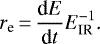
Because we applied this relation to monomers and clusters, N describes the total number of atoms in the given monomer or cluster. We used a fixed photon energy of EIR = 0.145 eV, which is equal to the energy of photons of the 8.6 μm feature. Finally, we computed the average photon-emission rate re by combining Eqs. (3) and (4) to obtain dE/dt and using
 (5)
(5)
2.2.3 Dissociation rates
To calculate the dissociation rates of a PAH cluster for single- and multi-photon processes, the individual rates were evaluated as a function of energy from an Arrhenius expression derived from the Rice–Ramsperger–Kassel–Marcus theory (RRKM theory). We followed the approach of Tielens (2005) and used
 (6)
(6)
with the entropy factor k0, the activation energy EA, Boltzmann’sconstant kB, and the effective temperature Te. Te can be calculated from the microcanonical temperature by adding a heat bath correction derived from the density of states, and it becomes
 (7)
(7)
For k0, we assumed a value of k0 = 2.5 × 10¹⁷ s−1 for all three PAH monomers, which is in agreement with the values given in Zacharia et al. (2004). A derivation of k0 can be found in the appendix. Instead of using the graphite exfoliation energy (Herdman & Miller 2008), we calculate the activation energy EA for PAH cluster dissociation by using an approximation from DFT calculations for the adsorption of PAHs onto graphene by Li et al. (2018),
 (8)
(8)
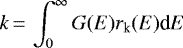
which is close to the approximation obtained from the experimental study of Zacharia et al. (2004). For our three considered molecules, this corresponds to EA = 1.4 eV for C24 H12, EA = 2.9 eV for C54 H18 and EA = 4.9 eV for C96 H24. The resulting dissociation rates for C24 H12, C54 H18, and C96 H24 dimers are displayed in Fig. 1 together with the IR photon-emission rate.
We accounted for the energy loss during dissociation by distributing the remaining energy of the cluster E′ = E − EA after break-up of one molecule equally into the degrees of freedom of the remaining daughter cluster and the separated monomer following
 (9)
(9)
where Ndau is the number of atoms in the daughter cluster and Nmon is the number of atoms in the monomer.
After one dissociation event, the cluster with Nmem member molecules has by definition changed its size and no longer belongs to the same sampled species. Strictly speaking, the energy probability distribution after dissociation needs to be taken into account to calculate the energy probability distribution of the species with one molecule less. This would require recursive calculations starting with the largest cluster while taking into account the local history of PAHs (multiple growth channels, dissociation). To properly sample it, a full cluster size evolution model is required. We have elected to ignore this change in the size of a dissociating PAH and assumed that larger clusters with Nmem + 1 monomers that fragment into the sampled cluster size with Nmem members have the same energy as the remaining energy of the daughter cluster with Nmem − 1 monomers after fragmentation from a cluster with Nmem monomers.
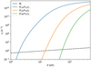 |
Fig. 1 Comparison of photodissociation rates obtained from Eq. (6) of PAH dimers and IR cooling rates dashed for the three simulated molecules coronene (blue), circumcoronene (orange), and circumcircumcoronene (green). The transition from IR cooling as the dominant energy-loss channel to photodissociation is sharp. |
2.2.4 Monte Carlo scheme
Our MC scheme follows the fundamental principles explained in Zsom & Dullemond (2008). Given the calculated rates described above, the total rate of events for a simulated PAH molecule is
 (10)
(10)
We determined a MC time step δt by drawing it randomly from an exponential distribution with mean 1∕r,
 (11)
(11)
To determine which event had occurred, we defined the set of all possible events with rates R = {ra,i, re, rk}. The probability of event j with rate rj ∈ R occurring is then
 (12)
(12)
Finally, the average dissociation rate of the simulated PAH cluster can be obtained from integration of the dissociation rate over the energy probability distribution5
 (13)
(13)
following Tielens (2005). We ran our MC model in blocks of 105 events and determined the energy probability distribution G(E) and the dissociation rate k after each block. When the standard deviation of the mean value for k was lower than 5%, we stopped our calculations. Otherwise, we sampled until we had simulated 2 × 10⁷ events. In these cases, the dissociation rate is very low and dominated by rare high-energy events, and the precise value is not astronomically relevant.
2.3 Statistical analysis
To confirm our MC results where the dissociation rate is very small, we performed a statistical analysis based on Purcell (1976), Bakes et al. (2001), and Andrews et al. (2016), for instance. Because cluster dissociation events are rare in these cases, they do not contribute significantly to the energy probability density. We therefore neglected energy loss due to dissociation in the statistical analysis.
Assuming that absorbed and emitted photons are Poisson distributed, the internal energy probability distribution G(E) can be described by
 (14)
(14)
where  is the average photon absorption rate,
  is derived from Eqs. (3) and (4), and τmin is the minimum time a PAH needs to cool from an excitation energy E1 to E. We considered the photon energy distribution in the same way as in the MC method by binning the spectrum.
  is then obtained by averaging G(E) over all photon energies Ei by
 (15)
(15)
Because we focus on multi-photon events in this analysis, the energy probability distribution Gn (E) has to be iteratively calculated with
 (16)
(16)
We set our initial energy probability distribution G1 to a Gaussian distribution around the radiative equilibrium energy Eeq with standard deviation σE to increase the convergence speed (see the appendix for an analytical approach and the derivation of Eeq and σE). When convergence was achieved, we calculated the cluster dissociation rate according to Eq. (13).
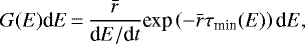
Figure 2 shows the energy probability distribution for a C96 H24 dimer obtained from the MC approach with cluster dissociation (blue) and without (orange). Dissociation leads to efficient cooling, and only a small fraction of time (high-energy tail) is spent at energies where cluster dissociation is dominant. Additionally, the critical energy Ecrit, where the probabilities for cooling and dissociation are equal, is indicated by the green probability curves. Internal energies between 50 eV and 60 eV become rare because they are results of cooling from higher energies. Because dissociation is dominant at high energies, the dimer does not continuously cool down, but instead loses half of its energy due to dissociation and is the origin of the shoulder at 30 eV.
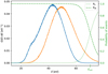 |
Fig. 2 Comparison of the energy probability distribution G(E) obtained from MC simulation (Herbig star model, 7.5 AU, (C96H24)2) with photodissociation (blue) and without photodissociation (orange). Additionally, the probability for photodissociation (green, dotted) and IR-cooling (green, dashed) are shown. With photodissociation, PAHs cool down so efficiently that only a smallfraction of time is spent at high temperatures. |
3 Disc model
In order to investigate the importance of clustering and cluster dissociation in protoplanetary discs, we set up two specific disc models. For our Herbig model, we chose HD169142 and for the T Tauri model BP Tau for direct comparison. We did not aim to model the observed discs in both systems with their features, but focused on taking the host stars as representative stars for Herbig and T Tauri stars, respectively, to study the effects of the radiative environment. We therefore applied a very general disc model. The stellar parameters for both stars are given in Table 1.
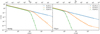 |
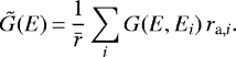
Fig. 3 Dimer dissociation rates obtained by MC simulations (crosses) for coronene (blue), circumcoronene (orange), and circumcircumcoronene (green) calculated with Eq. (13) with the stellar parameters given in Table 1. In both cases, coronene dimers can be dissociated with single-photon events. For larger molecules, the dissociation rate decreases tremendously with G0 when the radiative equilibrium energy drops below the critical energy. The multiple power-law fits (lines) are used for interpolation in Fig. 4. |
3.1 Disc profiles
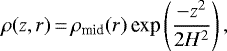
We applied our dissociation rate calculations to a protoplanetary disc with a surface density profile
 (17)
(17)
following a minimum mass solar nebula (MMSN) power-law profile as prescribed by Weidenschilling (1977). Our disc was set up so that the inner 100 AU contained a total mass of 0.01M*. We assumed a vertical gas density profile in hydrostatic equilibrium,
 (18)
(18)
where H denotes the gas pressure scale height given by H = cs∕ΩK and ρmid is calculated with 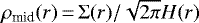 . The isothermal sound speed is given by the expression
 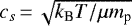 , where we assumed μ = 1.37. The disc follows an isothermal temperature profile in vertical direction,
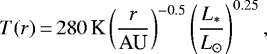 (19)
(19)
formulated by Hayashi (1981).
We furthermore assumed that the dust is well mixed with the gas and has a composition similar to that of the ISM to estimate the extinction caused by dust and gas in the disc. Our estimated value for the UV extinction cross section normalised to H atoms is σUV ≈ 10−21 cm2 per H atom (Ryter 1996). We determined the optical depth by integrating the hydrogen density along the line of sight. The extinction cross section depends on the grain size distribution and local dust-to-gas ratio. To estimate the effects of dust settling, we varied σUV by one order of magnitude in both directions to demonstrate the shifting of the τUV = 1 surface in the disc.
3.2 PAH monomer collisions
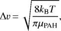
For our model we assumed that our disc gas and dust composition is similar to that of the ISM. We therefore used the proposed ratio of carbon atoms locked in PAHs to hydrogen atom that is obtained from the ISM CPAH : H = 1.5 × 10⁻⁵ given in Tielens (2008) to calculate number densities nPAH = n ⋅ 1.5 × 10⁻⁵∕NC of our simulated PAH molecules with NC C atoms from the hydrogen density n within the disc. We neglected PAH formation in the disc and assumed that all PAHs are primordial. Thermal motion is the only cause of collisions between two PAHs in the gas phase. The relative velocities between gas-phase PAH molecules can then be expressed by
 (20)
(20)
with μPAH being the reduced mass of two colliding PAH molecules and T being the kinetic temperature of the gas. Because our focus lies on collisions of individual PAH molecules, we assumed that PAH monomers are planar and their molecule radius can be expressed with 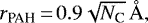 where NC is the number of carbon atoms in a monomer (Tielens 2008). The maximum geometrical collision cross section assuming parallel orientation for monomer-monomer interaction therefore is
 (21)
(21)
Finally, combining all expressions, the collision rate per PAH molecule is given by
 (22)
(22)
and we define the collision timescale per PAH molecule as
 (23)
(23)
All quantities in Eq. (22) depend on NC and are therefore PAH molecule specific.
4 Results
4.1 Formation and destruction of dimers
We wish to compare the PAH dimer dissociation timescale to the clustering timescale of monomers in our two disc models. Therefore we ran our MC scheme for several radiation field intensities G0 (in units of the mean Habing field) and computed the dissociation rates for coronene, circumcoronene, and circumcircumcoronene. Figure 3 shows the resulting dimer dissociation rates as a function of G0 and the corresponding distance from the star in the discs. The heat capacity of coronene dimers is small enough so that single photons heat the dimer above the critical energy Ecrit and trigger dissociation. The dissociation rate therefore decreases proportional to G0 and the squared distance. In contrast, circumcoronene and circumcircumcoronene dimers require multi-photon events and cannot be dissociated by individual photons. Close to the star, the radiative equilibrium energy is higher than Ecrit and the internal energy will strive through many photon absorptions towards Ecrit and finally dissociate the cluster. Consequently, the dissociation rate decreases linearly with G0 until Eeq drops below Ecrit in weaker radiation fields. The high-energy tail of G(E) then dominates the dissociation rate leading to a strong decrease given the exponential shape of the Arrhenius law. Additionally, the Lyman-alpha photons in the T Tauri disc are able to trigger single photon dissociation for coronene and circumcoronene. This contribution is negligible for coronene but relevant for circumcoronene and causes k to converge to a d−2 proportionality at distances larger than 100 AU. We fit the numerical values with analytical multiple power laws and applied the fit values to the disc model.
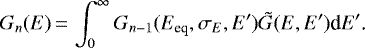
Figure 4 shows a comparison between the PAH monomer collision timescale (filled contours) and the PAH dimer dissociation timescale (black contours, same units) for the three simulated monomers coronene (C24H12), circumcoronene (C54H18), and circumcircumcoronene (C96H24). In all cases, the collision timescale for monomers is significantly shorter, about some secondsto years, than the typical lifetime of a disc of a few million years (Haisch et al. 2001). There is no significant difference of monomer collision rates between the Herbig star disc and the T Tauri star disc. In contrast, the dissociation timescale for dimers differs between the Herbig model and the T Tauri model. Because of the higher luminosity and the more energetic photons, the dissociation timescale in the Herbig model is several orders of magnitude lower than for the T Tauri model. While coronene and circumcoronene can be dissociated in less than a year within the innermost 100 AU, circumcircumcoronene cannot be dissociated beyond 50 AU in the Herbig model and 7 AU in the T Tauri model.
Optical depth was not considered in deriving the cluster dissociation timescales. For further analysis, we indicate the estimated τUV = 1 surface for several effective absorption cross sections (red, blue, and green lines) to separate the disc into the photosphereand the sub-photospheric layer. In this simple separation, the photosphere will mostly be dominated by dissociation events. Only for circumcircumcoronene in the Herbig model beyond 20 AU, collisions occur at a higher rate than dissociation. For the T Tauri model, circumcoronene and circumcircumcoronene monomer collisions will occur faster than a dimer dissociates beyond 30 AU resp. 2 AU. The sub-photospheric layers are collision dominated and allow cluster to grow beyond the dimer stage because of the high collision rate. We further wish to analyse the stability of PAH clusters as a function of cluster size given that the collision timescales are rather short.
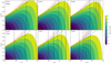 |
Fig. 4 Comparison between collision timescale of monomers (filled contours) and dissociation timescale of dimers (black contours, same units) for the Herbig model (top row) and the T Tauri model (bottom row). Left: coronene, middle: circumcoronene, and right: circumcircumcoronene. Estimated τUV = 1 surfaces are indicated by coloured lines. Monomer collisions occur in all cases on disc-relevant timescales within 100 AU below the τ = 1 surfaces. |
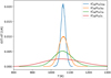 |
Fig. 5 Temperature probability distribution in the same environment (d = 12.5 AU in HD169142) for different circumcircumcoronene clusters. With growing size, temperature fluctuations decrease because of a higher photon absorption rate and the dissociation rate converges towards the value at the radiative equilibrium temperature. |
4.2 PAH cluster size effects
To investigate the stability of larger cluster, we performed our MC calculations for clusters with up to 200 monomers and tracked the dissociation rates for both discs and all three PAH molecules. Given that the heat capacity increases approximately linear with the number of carbon atoms in a cluster and each carbon atom absorbs the same amount of energy, clusters have the same radiative equilibrium temperature independent of size. Therefore it is more practical to present temperatures instead of internal energies to explain the effects on the dissociation rate. Depending on the radiation field intensity, a growing cluster can either increase its stability if Teq < Tcrit or, in contrast, weaken it if Teq > Tcrit.
In the first case, where Teq < Tcrit, single-photon events become very unlikely for larger clusters and the dissociation rate is entirely dominated by the temperature probability distribution. Figure 5 shows the temperature probability distribution for growing circumcircumcoronene clusters in the same radiative environment where the radiative equilibrium temperature is lower than the critical temperature. While a tetramer undergoes large temperature fluctuations, larger clusters have narrower temperature distributions, with the maximum located at the radiative equilibrium value of Teq = 1073 K corresponding to Eeq,4 = 71 eV, Eeq,16 = 286 eV, Eeq,64 = 1144 eV, and Eeq,256 = 4578 eV for the clusters shown and approximated by the analytical formulas given in Appendix B.
The larger the cluster, the shorter the time interval between photon absorptions and the lower the degree of temperature fluctuations.Because high-temperature events become less likely the larger the cluster, the dissociation rate decreases and converges towards the radiative equilibrium value. In addition, the greatest increase in stability is gained by the smallest clusters.
Conversely, at smaller distances, where Teq > Tcrit, clusters undergo dissociation before the equilibrium temperature can be reached. After an initial dissociation event, the time until the next dissociation is determined by the time it takes to compensate for the energy loss of the previous dissociation. The smaller the cluster, the more energy is lost by release of a monomer relative to the total energy of the cluster (see Eq. (9)). However, the absorbed energy flux is proportional to the number of molecules inthe cluster, and therefore smaller clusters need longer to compensate for the energy loss. This means that clusters cannot be stabilised in very strong radiation fields and are even faster dissociated the larger they are.
Figure 6 shows the dissociation timescale as a function of cluster size for circumcircumcoronene in the T Tauri model. Following the idea of Siebenmorgen & Krügel (2010), we wish to compare our dissociation rates to the vertical mixing timescale at a given distance. We estimate the local eddy timescale ted similar to Dullemond & Dominik (2004) with q = 0.5 by
 (24)
(24)
where α is the alpha viscosity parameter first described by Shakura & Sunyaev (1973) and Ωk is the local Keplerian orbital velocity. Where mixing is faster than dissociation (τk > ted), the coloured lines transition from green to black. We call these clusters stable, implying that a fraction of the clusters is able to survive. The dissociation rates for very large clusters are noted as circles. At small distances, clusters do not gain stability by increasing cluster size and undergo cascade dissociation events in a short period of time. Although dissociation still occurs on short timescales at 1 AU, clusters will gain stability with larger sizes because Teq declines below Tcrit so that the dissociation is entirely fluctuation dominated. Then, the dissociation timescale will approach the value at equilibrium temperature for growing clusters. Outside 2 AU, circumcircumcoronene dimers are stable. The full diagram with all simulated PAHs for both disc models can be found in the appendix (Fig. C.1).
To summarise our results, we tracked the cluster size where ted = τk(Ncrit) for all simulated PAHs and distances. Figure 7 shows the critical cluster size as a function of distance when exposed to the full stellar flux. The filled colour represents the smallest PAH that is stable at a given distance. The transition from unstable to stable of dimers occurs over a short distance for circumcircumcoronene. Circumcoronene can be stabilised but needs to grow beyond dimers in most parts of the discs. The smallest molecule, coronene, needs at least 30 cluster members to gain stability in the outer parts of the disc. For the Herbig model, no cluster is expected to survive in the innermost 20 AU, regardless of size and PAH. In the T Tauri model, no cluster can survive within 1.5 AU.
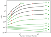 |
Fig. 6 Dissociation timescale for circumcircumcoronene clusters in the T Tauri model. Solid lines: MC simulations. Crosses: statistical calculations. Circles: value at radiative equilibrium temperature. The transition from green to black denotes the cluster size at which the vertical mixing timescale equals the dissociation timescale. Up to 0.9 AU, the radiative equilibrium temperature is higher than the critical temperature for dissociation and cluster cannot gain stability. At larger distances, cluster stability increases with a few more cluster member. |
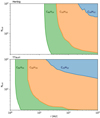 |
Fig. 7 Critical number of cluster members where ted = τk for the Herbig model (top, lines) and the T Tauri model (bottom, lines). The smallest stable molecule is indicated by the filled colour. For the Herbig star model, clusters are stable outside the regions where they can possibly form. In the T Tauri disc model, circumcoronene and circumcircumcoronene can be stabilised where clusters can form in the midplane. Coronene clusters are unlikely to survive. |
5 Discussion
In our studywe find that PAH cluster formation can occur within years in the entire disc if the cluster is shielded from stellar radiation. Studies have reported that PAH clusters gain additional vibrational lines (Rapacioli et al. 2007) and may be associated with the broad non-continuum plateaus underlying the PAH feature emission (Bregman et al. 1989; Rapacioli et al. 2005b). PAH abundance measurements such as those of Acke et al. (2010) are based on the extraction of sharp PAH features. Under the condition that PAH clusters are mixed from the midplane into the photosphere and survive, they could contribute to the underlying continuum, and PAH feature flux studies might underestimate the total amount of PAH molecules in the protoplanetary disc. We therefore wish to discuss this possibility in connection with our results.
5.1 Herbig model
The comparison of the cluster formation and the stability of clusters (Fig. 7) shows that coronene and circumcoronene clusters will break up within a short time when exposed to the full stellar radiation and do not survive. Circumcircumcoronene cluster are able to withstand the stellar radiation outside 25 AU by forming dimers, and circumcoronene quadrumers can withstand the stellar radiation beyond 100 AU. These sizes can be reached within several years. We therefore expect clusters to be present in the photosphere at large distances. As HD169142 is on the cooler and less luminous end of the Herbig stars, the dissociation rates can be treated as a lower limit for the Herbig stars. We therefore conclude that PAHs are prominently present as monomers in the inner disc photosphere. We cannot rule out that cluster formation can explain that no PAH emission is detected in 40% of Herbig star discs, but consider this scenario unlikely. An alternative explanation for the missing PAH flux is likely the high UV flux that causes PAH monomers to be irreversibly destroyed and deplete PAHs in discs.
5.2 T Tauri model
In contrast to the Herbig model, PAH clusters can be stabilised at small radii in the T Tauri disc if they have the size of circumcoronene. Based on the monomer collision rate, clusters can grow to this size within several years. These clusters would be stable to the stellar radiation and could grow further even if exposed to stellar radiation. This means that the formation of PAH clusters can be one possible explanation why only 10% of T Tauri discs show PAH features. In the literature, attenuation and lack of excitation emission have been excluded, while cluster formation and trapping of PAHs in ices have been raised as possible explanations by Geers et al. (2009). Cluster formation and desorption onto dust grains are competing in the sub-photospheric layers. To trace the importance of these two processes, a PAH time-evolution model is required that takes collisions between PAHs and dust grains into account. Furthermore, with a time-evolution model, cluster growth could be tracked and linked to the strength of vertical mixing. We will consider these processes in a future study.
Furthermore, our derived dissociation rates can be extrapolated to desorption of PAHs from dust grains. When we consider dust grains as very large clusters at radiative equilibrium temperature, then the rate at which PAH monomers detach from the surface of a grain is given by the equilibrium rate indicated by circles in Figs. 6 and C.1. When a PAH cluster of any size is stable, individual PAHs will therefore also stay adsorbed on dust grain surfaces. This approximation might also be valid for small PAH clusters, but for larger sizes, PAH clusters will likely behave like small grains rather than individual molecules. Interpreting Fig. 7, adsorption of PAHs is more important for T Tauri star discs than for Herbig star discs.
In our study, we made multiple approximations, and here we discuss their effect on our results. Instead of calculating the emission probabilities for each PAH band at all temperatures, we decided to use a simplified approach by directly using the cooling law obtained by the emission model of Bakes et al. (2001) and a constant IR photon energy. Because we calculated the emission rate directly from the cooling law, the choice of the emission photon energy is arbitrary, but sets the resolution and noise level of the resulting energy distribution. Higher photon energies reduce the noise level of G(E) at the cost of lower resolution, while lower photon energies have the reverse effect. We find that the choice EIR in the range of physical PAH bands affects the computed dissociation rate only moderately; the rate is mostly dominated by the MC noise at the very rare high energies.
Furthermore, we assumed in Sect. 2.2.3 that a cluster dissociating from size Nmem has a similar energy as a cluster of size Nmem + 1 after dissociation. This approximation holds well for large clusters that are close to radiative equilibrium because their absolute energy loss due to dissociation becomes almost constant. Our approximation deteriorates for smaller clusters because the relative energy loss is proportional to Nmem∕(Nmem + 1). We therefore overestimate the relative energy loss from dissociation by  and underestimate the dissociation rate. For a dimer formed from dissociating a trimer, the relative energy difference is 25%. The resulting change in the dissociation rate is difficult to estimate because of the exponential behaviour of the Arrhenius law and because the previous dissociation event is only a fraction of the total energy probability distribution. Nevertheless, this effect is only strong when the PAHs undergo quick cascading dissociation. In these cases, the dissociation rate is very high and dominates clustering. Therefore uncertainties in the dissociation timescale do not affect the long-term evolution of PAH clusters.
In Eq. (8), we have to assume the binding energy of a monomer to a cluster that is usedfor all cluster sizes. As stated before, because of the exponential dependence on EA, small changes in EA can have large effects on the dissociation rate at a given energy. We find that a deviation of ±10% in EA can change the local dissociation rate by a factor two for very high dissociation rates (k ≈ 1 s−1) to two orders of magnitude when the dissociation rate is low (k ≈ 10−13 s−1), depending on the exact simulation configuration including cluster size, PAH species, and radiation field. Although this is locally a huge effect, the steep gradient of k(r) rapidly compensates for this. A decrease in dissociation rate by two orders of magnitudes in Figs. 6 and C.1 corresponds to a maximum increase in distance of 50 AU for large coronene clusters in the Herbig model and a minimum increase of 0.2 AU for large circumcircumcoronene clusters in the T Tauri model. Compared to the individual distances where cluster stability is achieved in our conclusion Fig. 7, this corresponds to a maximum shift for coronene in the Herbig model from 200 AU to 250 AU and a minimum shift from 1.5 to 1.7 AU for circumcircumcoronene in the T Tauri model.
For a full time-evolution model we wish to discuss further processes that it is relevant to include but that we did not consider. As reported by Siebenmorgen & Krügel (2010), the X-ray excess of T Tauri stars is an additional energy source and can penetrate deeper into the disc than UV radiation (Ryter 1996). The absorption of X-rays by PAHs has been studied in the laboratory, for example, by Reitsma et al. (2014). Furthermore, their secondary effects as well as secondary effects of cosmic rays can locally produce additional UV photons in the sub-photospheric layers (Tielens 2005), which can potentially destroy small PAH clusters through single-photon dissociation.
In our analysis of the photo fragmentation, we assumed that IR emission is the only stabilising process. However, for large PAHs, the monomer binding energy approaches that of covalent bonds of C–H, for example. To compare our derived rates for dimers (Fig. 1) to the dehydrogenation rates for monomers obtained by Andrews et al. (2016), we need to extrapolate their internal energies by multiplication with a factor 2 to correct for the additional degrees of freedom of the dimer. While coronene and circumcoronene dimers will dissociate rather than release H or H2, circumcircumcoronene will break H-C bonds before a dimer will dissociate. For high atomic H densities, for instance, in the upper photosphere, dehydrogenation-hydrogenation cycles would act to stabilise clusters made of large PAHs.
Lastly, ionisation has not been considered so far. Typical ionisation potentials for neutral PAH monomers are of about 5–7 eV (Tielens 2005). Joblin et al. (2017) reported decreasing ionisation potentials for growing PAH clusters. Rapacioli & Spiegelman (2009) reported that the activation energy for dissociation of small, ionised clusters is significantly higher than that of neutral clusters. Therefore, ionisation can support the stability of PAH cluster by competing with dissociation while increasing the energy needed to dissociate ionised clusters especially for small clusters that are dominantly dissociated by single-photon events. As a side effect, ionisation decreases the probability of reaching higher energies in PAHs that experience large energy fluctuations, reducing the strength of the short-wavelength emission. This requires a sufficient number of free electrons to recombine in order to keep the neutral fraction high and is probably limited to small regions in a protoplanetary disc. Whether these processes support cluster survivability in the photosphere of Herbig and T Tauri stars needs to be investigated in a future study.
6 Conclusions
We have presented calculations for cluster formation of PAHs under protoplanetary disc conditions for a Herbig Ae/Be disc model and a T Tauri disc model assuming a pristine PAH abundance similar to the ISM. We reported that dimer formation occurs on timescales much shorter than a disc lifetime for molecules of astrophysical relevance in the sub-photospheric layers of protoplanetary discs. Clusters are unlikely to survive in the inner disc photosphere and need to be carried to the photosphereby vertical mixing or other processes. We further provided calculations for the dissociation rates of different cluster sizes depending on the radiation field intensity. For the Herbig star disc model, clusters are unlikely to survive because of the strong stellar radiation if no other energy-loss channel other than IR emission is considered. Under these conditions, cluster formation is unlikely to be the reason why 40% of Herbig stars do not show PAH emission. For the T Tauri disc model, PAHs as large as circumcoronene or larger are able to form clusters that can withstand the stellar UV radiation. We propose PAH cluster formation as one possible explanation for the lack of PAH emission in most T Tauri discs. For further investigation, a more sophisticated PAH evolution model has to be developed that takes processes competing with dissociation into account, such as ionisation and dehydrogenation.
Acknowledgements
The authors thank the anonymous referee for suggestions to improve the quality of the paper. K.L. acknowledges funding from the Nederlandse Onderzoekschool Voor Astronomie (NOVA) project number R.2320.0130. C.D. acknowledges funding from the Netherlands Organisation for Scientific Research (NWO) TOP-1 grant as part of the research program “Herbig Ae/Be stars, Rosetta stones for understanding the formation of planetary systems”, project number 614.001.552. Studies of interstellar PAHs at Leiden Observatory are supported through a Spinoza award from the Dutch research council, NWO.
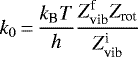
Appendix A Derivation of k0
The derivation of the pre-exponential factor k0 for the Arrhenius law for the dissociation of a single molecule from a cluster is based on Tielens (2005) and Tielens (2021). From thermodynamics, the rate constant can be expressed with
 (A.1)
(A.1)
assuming a monoatomic gas. kb describes Boltzmann’s constant, T is the temperature, h is Planck’s constant, and Z describes the vibrational and rotational partition functions. We assumed that only one molecule can detach fromthe cluster at a time and that the number of degrees of freedom by the breakup of the cluster stays constant. When we consider only the perpendicular mode for excitation, we can write k0 as
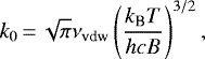 (A.2)
(A.2)
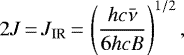
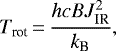
where νvdw is the frequency of the van der Waals bond and B is the rotational constant. Knowing that ΔJ = +1 and ΔJ = −1 transitions during an de-excitation cascade are balanced leads to
 (A.3)
(A.3)
with  being the typical IR photon energy. Together with the rotational excitation temperature
 (A.4)
(A.4)
which finally leads to
 (A.5)
(A.5)
Using typical values for PAHs of νvdw = 50 – 70 cm−1 results in k0 = 2.5 × 10¹⁷ s−1.
Appendix B Analytical calculation of G(E)
When the photodissociation rate is low and the photon absorption rate is sufficiently high (τUV≫̸τcool), the energy probability distribution can be approximated by a Gaussian distribution (Tielens 2021) that is a result of the Poissonian character of photon absorption. The accuracy of this approach increases the closer the cluster is to the radiative equilibrium and the smaller the energy fluctuations. Then, the mean of the distribution is equal to the radiative equilibrium energy Eeq given by
 (B.1)
(B.1)
where  is the mean uv photon energy and
  is the equivalent mean photon absorption rate. The Gaussian standard deviation σ can be calculated with
 (B.2)
(B.2)
κ is an empirical correction factor necessary to account for the non-Poissonian characteristic of the cooling law. The correction factor is dependent on the exact shape of the cooling law. We found a suitable value of κ ≈ 6∕11 for our simulated cases. Unfortunately, this relation is not suitable to evaluate Eq. (13) for small clusters because of the asymmetrical character of G(E) and the exponential dependence of k on the energy.
Appendix C Fitting parameters for k(d)
All data points in Fig. 3 are fitted in logarithmic space with linear functions of shape
 (C.1)
(C.1)
which corresponds to
 (C.2)
(C.2)
in linear space using k in s and d in AU. The individual power laws are connected similarly to Eq. (4), where the power has to be adjusted by hand to match the correct shape.
 |
Fig. C.1 Full plot for Fig. 6. Top row: Herbig model. Bottom row: T Tauri model. From left to right: coronene, circumcoronene, and circumcircumcoronene. Solid lines: values obtained from MC-simulations. Crosses: values obtained from statistical calculations. The transition from coloured lines to black shows the cluster size at which the dissociation timescale of the cluster equals the eddy turnover timescale. We consider the black lines to be stable. The smaller the monomer molecule, the larger the distances required to reach stability and the smaller the stability gain per member molecule. Coronene is too small to be stabilised over 1000 AU in both discs. |
References
- Acke, B., & van den Ancker, M. E. 2004, A&A, 426, 151 [NASA ADS] [CrossRef] [EDP Sciences] [Google Scholar]
- Acke, B., Bouwman, J., Juhász, A., et al. 2010, ApJ, 718, 558 [NASA ADS] [CrossRef] [Google Scholar]
- Allamandola, L. J., Tielens, A. G. G. M., & Barker, J. R. 1989, ApJS, 71, 733 [Google Scholar]
- Andrews, H., Candian, A., & Tielens, A. G. G. M. 2016, A&A, 595, A23 [NASA ADS] [CrossRef] [EDP Sciences] [Google Scholar]
- Bakes, E. L. O., & Tielens, A. G. G. M. 1994, ApJ, 427, 822 [NASA ADS] [CrossRef] [Google Scholar]
- Bakes, E. L. O., Tielens, A. G. G. M., & Bauschlicher, Charles W., J. 2001, ApJ, 556, 501 [NASA ADS] [CrossRef] [Google Scholar]
- Bregman, J. D., Allamandola, L. J., Tielens, A. G. G. M., Geballe, T. R., & Witteborn, F. C. 1989, ApJ, 344, 791 [NASA ADS] [CrossRef] [PubMed] [Google Scholar]
- Cami, J., Bernard-Salas, J., Peeters, E., & Malek, S. E. 2010, Science, 329, 1180 [NASA ADS] [CrossRef] [PubMed] [Google Scholar]
- Croiset, B. A., Candian, A., Berné, O., & Tielens, A. G. G. M. 2016, A&A, 590, A26 [NASA ADS] [CrossRef] [EDP Sciences] [Google Scholar]
- Doucet, C., Habart, E., Pantin, E., et al. 2007, A&A, 470, 625 [CrossRef] [EDP Sciences] [Google Scholar]
- Dullemond, C. P., & Dominik, C. 2004, A&A, 421, 1075 [NASA ADS] [CrossRef] [EDP Sciences] [Google Scholar]
- Geers, V. C., Augereau, J. C., Pontoppidan, K. M., et al. 2006, A&A, 459, 545 [NASA ADS] [CrossRef] [EDP Sciences] [Google Scholar]
- Geers, V. C., van Dishoeck, E. F., Visser, R., et al. 2007, A&A, 476, 279 [NASA ADS] [CrossRef] [EDP Sciences] [Google Scholar]
- Geers, V. C., van Dishoeck, E. F., Pontoppidan, K. M., et al. 2009, A&A, 495, 837 [NASA ADS] [CrossRef] [EDP Sciences] [Google Scholar]
- Grankin, K. N. 2016, Astron. Lett., 42, 314 [NASA ADS] [CrossRef] [Google Scholar]
- Haisch, Karl E., J., Lada, E. A., & Lada, C. J. 2001, ApJ, 553, L153 [Google Scholar]
- Hayashi, C. 1981, Progr. Theor. Phys. Suppl., 70, 35 [Google Scholar]
- Herdman, J. D., & Miller, J. H. 2008, J. Phys. Chem. A, 112, 6249 [CrossRef] [Google Scholar]
- Honda, M., Maaskant, K., Okamoto, Y. K., et al. 2012, ApJ, 752, 143 [Google Scholar]
- Hony, S., Van Kerckhoven, C., Peeters, E., et al. 2001, A&A, 370, 1030 [NASA ADS] [CrossRef] [EDP Sciences] [Google Scholar]
- Joblin, C., Dontot, L., Garcia, G. A., et al. 2017, J. Phys. Chem. Lett., 8, 3697 [NASA ADS] [CrossRef] [Google Scholar]
- Lagage, P.-O., Doucet, C., Pantin, E., et al. 2006, Science, 314, 621 [NASA ADS] [CrossRef] [PubMed] [Google Scholar]
- Leger, A., & Puget, J. L. 1984, A&A, 500, 279 [NASA ADS] [Google Scholar]
- Li, B., Ou, P., Wei, Y., Zhang, X., & Song, J. 2018, Materials, 11, 726 [NASA ADS] [CrossRef] [Google Scholar]
- Malloci, G., Joblin, C., & Mulas, G. 2007, Chem. Phys., 332, 353 [Google Scholar]
- Menéndez, J., & Page, J. B. 2000, Vibrational spectroscopy of C60, ed. M. Cardona, & G. Güntherodt, 76, 27 [Google Scholar]
- Peeters, E., Hony, S., Van Kerckhoven, C., et al. 2002, A&A, 390, 1089 [NASA ADS] [CrossRef] [EDP Sciences] [Google Scholar]
- Purcell, E. M. 1976, ApJ, 206, 685 [NASA ADS] [CrossRef] [Google Scholar]
- Raj, A., Sander, M., Janardhanan, V., & Kraft, M. 2010, Combust. Flame, 157, 523 [Google Scholar]
- Rapacioli, M., & Spiegelman, F. 2009, Eur. Phys. J. D, 52, 55 [NASA ADS] [CrossRef] [EDP Sciences] [Google Scholar]
- Rapacioli, M., Calvo, F., Spiegelman, F., Joblin, C., & Wales, D. J. 2005a, J. Phys. Chem. A, 109, 2487 [CrossRef] [PubMed] [Google Scholar]
- Rapacioli, M., Joblin, C., Boissel, P., Calvo, F., & Spiegelman, F. 2005b, in ESA SP, 577, ed. A. Wilson, 409 [NASA ADS] [Google Scholar]
- Rapacioli, M., Calvo, F., Joblin, C., et al. 2006, A&A, 460, 519 [NASA ADS] [CrossRef] [EDP Sciences] [Google Scholar]
- Rapacioli, M., Calvo, F., Joblin, C., Parneix, P., & Spiegelman, F. 2007, J. Phys. Chem. A, 111, 2999 [CrossRef] [PubMed] [Google Scholar]
- Reitsma, G., Boschman, L., Deuzeman, M. J., et al. 2014, Phys. Rev. Lett., 113, 053002 [NASA ADS] [CrossRef] [PubMed] [Google Scholar]
- Rodenkirch, P. J., Klahr, H., Fendt, C., & Dullemond, C. P. 2020, A&A, 633, A21 [CrossRef] [EDP Sciences] [Google Scholar]
- Ryter, C. E. 1996, Ap&SS, 236, 285 [NASA ADS] [CrossRef] [Google Scholar]
- Sander, M., Patterson, R. I., Braumann, A., Raj, A., & Kraft, M. 2011, Proc. Combust. Inst., 33, 675 [Google Scholar]
- Sellgren, K., Werner, M. W., Ingalls, J. G., et al. 2010, ApJ, 722, L54 [NASA ADS] [CrossRef] [Google Scholar]
- Shakura, N. I., & Sunyaev, R. A. 1973, A&A, 500, 33 [NASA ADS] [Google Scholar]
- Siebenmorgen,R., & Heymann, F. 2012, A&A, 543, A25 [NASA ADS] [CrossRef] [EDP Sciences] [Google Scholar]
- Siebenmorgen,R., & Krügel, E. 2010, A&A, 511, A6 [NASA ADS] [CrossRef] [EDP Sciences] [Google Scholar]
- Tielens, A. G. G. M. 2005, Physics and Chemistry of the Interstellar Medium [Google Scholar]
- Tielens, A. G. G. M. 2008, ARA&A, 46, 289 [NASA ADS] [CrossRef] [EDP Sciences] [Google Scholar]
- Tielens, A. G. G. M. 2021, Molecular Astrophysics (Cambridge University Press) [Google Scholar]
- Weidenschilling, S. J. 1977, Ap&SS, 51, 153 [Google Scholar]
- Zacharia, R., Ulbricht, H., & Hertel, T. 2004, Phys. Rev. B, 69, 155406 [NASA ADS] [CrossRef] [Google Scholar]
- Zsom, A., & Dullemond, C. P. 2008, A&A, 489, 931 [NASA ADS] [CrossRef] [EDP Sciences] [Google Scholar]
See e.g. the PAH IR spectral database for an overview of PAH molecules https://www.astrochemistry.org/pahdb/
Available at https://www.dsf.unica.it/gmalloci/pahs/pahs.html
We do not bin in wavelength space to ensure a linear step size in the energy grid.
In order to preserve differentiability at the transition we use the smoothening relation
 . We have tested both shallower and steeper power laws and find that this relation is the best compromise between smoothness and deviation from the original curves around the transition point.
The dissociation rate can also be obtained from counting the dissociation events, but the integral is more stable against MC noise.
All Tables
All Figures
|
Fig. 1 Comparison of photodissociation rates obtained from Eq. (6) of PAH dimers and IR cooling rates dashed for the three simulated molecules coronene (blue), circumcoronene (orange), and circumcircumcoronene (green). The transition from IR cooling as the dominant energy-loss channel to photodissociation is sharp. |
| In the text | |
|
Fig. 2 Comparison of the energy probability distribution G(E) obtained from MC simulation (Herbig star model, 7.5 AU, (C96H24)2) with photodissociation (blue) and without photodissociation (orange). Additionally, the probability for photodissociation (green, dotted) and IR-cooling (green, dashed) are shown. With photodissociation, PAHs cool down so efficiently that only a smallfraction of time is spent at high temperatures. |
| In the text | |
|
Fig. 3 Dimer dissociation rates obtained by MC simulations (crosses) for coronene (blue), circumcoronene (orange), and circumcircumcoronene (green) calculated with Eq. (13) with the stellar parameters given in Table 1. In both cases, coronene dimers can be dissociated with single-photon events. For larger molecules, the dissociation rate decreases tremendously with G0 when the radiative equilibrium energy drops below the critical energy. The multiple power-law fits (lines) are used for interpolation in Fig. 4. |
| In the text | |
|
Fig. 4 Comparison between collision timescale of monomers (filled contours) and dissociation timescale of dimers (black contours, same units) for the Herbig model (top row) and the T Tauri model (bottom row). Left: coronene, middle: circumcoronene, and right: circumcircumcoronene. Estimated τUV = 1 surfaces are indicated by coloured lines. Monomer collisions occur in all cases on disc-relevant timescales within 100 AU below the τ = 1 surfaces. |
| In the text | |
|
Fig. 5 Temperature probability distribution in the same environment (d = 12.5 AU in HD169142) for different circumcircumcoronene clusters. With growing size, temperature fluctuations decrease because of a higher photon absorption rate and the dissociation rate converges towards the value at the radiative equilibrium temperature. |
| In the text | |
|
Fig. 6 Dissociation timescale for circumcircumcoronene clusters in the T Tauri model. Solid lines: MC simulations. Crosses: statistical calculations. Circles: value at radiative equilibrium temperature. The transition from green to black denotes the cluster size at which the vertical mixing timescale equals the dissociation timescale. Up to 0.9 AU, the radiative equilibrium temperature is higher than the critical temperature for dissociation and cluster cannot gain stability. At larger distances, cluster stability increases with a few more cluster member. |
| In the text | |
|
Fig. 7 Critical number of cluster members where ted = τk for the Herbig model (top, lines) and the T Tauri model (bottom, lines). The smallest stable molecule is indicated by the filled colour. For the Herbig star model, clusters are stable outside the regions where they can possibly form. In the T Tauri disc model, circumcoronene and circumcircumcoronene can be stabilised where clusters can form in the midplane. Coronene clusters are unlikely to survive. |
| In the text | |
|
Fig. C.1 Full plot for Fig. 6. Top row: Herbig model. Bottom row: T Tauri model. From left to right: coronene, circumcoronene, and circumcircumcoronene. Solid lines: values obtained from MC-simulations. Crosses: values obtained from statistical calculations. The transition from coloured lines to black shows the cluster size at which the dissociation timescale of the cluster equals the eddy turnover timescale. We consider the black lines to be stable. The smaller the monomer molecule, the larger the distances required to reach stability and the smaller the stability gain per member molecule. Coronene is too small to be stabilised over 1000 AU in both discs. |
| In the text | |
Current usage metrics show cumulative count of Article Views (full-text article views including HTML views, PDF and ePub downloads, according to the available data) and Abstracts Views on Vision4Press platform.
Data correspond to usage on the plateform after 2015. The current usage metrics is available 48-96 hours after online publication and is updated daily on week days.
Initial download of the metrics may take a while.