| Issue |
A&A
Volume 652, August 2021
|
|
|---|---|---|
| Article Number | A117 | |
| Number of page(s) | 8 | |
| Section | Planets and planetary systems | |
| DOI | https://doi.org/10.1051/0004-6361/202140768 | |
| Published online | 19 August 2021 | |
A search for transiting companions in the J1407 (V1400 Cen) system★
1
Leiden Observatory, University of Leiden, PO Box 9513,
2300
RA Leiden,
The Netherlands
e-mail: This email address is being protected from spambots. You need JavaScript enabled to view it.
2
Jet Propulsion Laboratory, California Institute of Technology, 4800 Oak Grove Drive, M/S 321-100,
Pasadena,
CA
91109,
USA
3
Department of Physics & Astronomy, University of Rochester,
Rochester,
NY
14627,
USA
4
American Association of Variable Star Observers (AAVSO), 49 Bay State Rd.,
Cambridge,
MA
02138,
USA
5
Vereniging Voor Sterrenkunde (VVS), Oostmeers 122 C,
8000
Brugge,
Belgium
6
Department of Physics and Astronomy, University of North Carolina at Chapel Hill, Campus Box 3255,
Chapel Hill,
NC
27599,
USA
7
Department of Physics and Astronomy, Michigan State University,
East Lansing,
MI
48824,
USA
Received:
9
March
2021
Accepted:
17
June
2021
Abstract
Context. In 2007, the young star 1SWASP J140747.93-394 542.6 (V1400 Cen) underwent a complex series of deep eclipses over 56 days. This was attributed to the transit of a ring system filling a large fraction of the Hill sphere of an unseen substellar companion. Subsequent photometric monitoring has not found any other deep transits from this candidate ring system, but if there are more substellar companions and if they are coplanar with the potential ring system, there is a chance that they will transit the star as well. This young star is active, and the light curves show a 5% modulation in amplitude with a dominant rotation period of 3.2 days due to starspots rotating into and out of view.
Aims. We model and remove the rotational modulation of the J1407 light curve and search for additional transit signatures of substellar companions orbiting around J1407.
Methods. We combine the photometry of J1407 from several observatories, spanning a 19 yr baseline. We remove the rotational modulation by modeling the variability as a periodic signal, whose periodicity changes slowly with time over several years due to the activity cycle of the star. A transit least squares (TLS) analysis is used to search for any periodic transiting signals within the cleaned light curve.
Results. We identify an activity cycle of J1407 with a period of 5.4 yr. A TLS search does not find any plausible periodic eclipses in the light curve, from 1.2% amplitude at 5 days up to 1.9% at 20 days. This sensitivity is confirmed by injecting artificial transits into the light curve and determining the recovery fraction as a function of transit depth and orbital period.
Conclusions. J1407 is confirmed as a young active star with an activity cycle consistent with a rapidly rotating solar mass star. With the rotational modulation removed, the TLS analysis reaches down to planetary mass radii for young exoplanets, ruling out transiting companions with radii larger than about 1 RJup.
Key words: planets and satellites: rings / stars: activity / dynamo / planets and satellites: detection
Processed photometric data are only available at the CDS via anonymous ftp to cdsarc.u-strasbg.fr (130.79.128.5) or via http://cdsarc.u-strasbg.fr/viz-bin/cat/J/A+A/652/A117
The first two authors contributed equally to this work.
© ESO 2021
1 Introduction
Ring systems are a ubiquitous feature in planetary systems – all the gas giants in the Solar System have ring systems around them of varying optical depths (see, e.g., Tiscareno 2013; Charnoz et al. 2018), and ring systems have been detected around minor planets (e.g., Chariklo; Braga-Ribas et al. 2014), so it is reasonable that exoplanets and substellar objects host ring systems as well. Long-period eclipsing binary star systems, where one star is surrounded by an extended dark disk-like structure that periodically eclipses the other component, have already been observed, such as EE Cep (Mikolajewski & Graczyk 1999), ϵ Aurigae (Guinan & Dewarf 2002), and TYC 2505-672-1, with a companion period of 69 yr (Lipunov et al. 2016; Rodriguez et al. 2016). A large ring-like structure around a substellar companion was proposed to explain observations from 2007 from the J1407 system (Mamajek et al. 2012). 1SWASP J140747.93-394 542.6 (V1400 Cen; hereafter called “J1407”) is a young, pre-main-sequence star in the Sco-Cen OB association (Mamajek et al. 2012) with spectral type K5 IV(e) Li and is similar in size and mass to the Sun. In 2007, it displayed a complex symmetric dimming pattern of up to ~ 3 magnitudes during a 56 day eclipse. This has been attributed to the transit of a substellar companion (called “J1407 b”) with a mass of 60–100 MJup (Rieder & Kenworthy 2016) surrounded by an exoring system consisting of at least 37 rings and extending out to 0.6 au in radius (Kenworthy & Mamajek 2015). For these rings to show detectable transit signatures, they must be significantly misaligned with respect to the orbital plane of J1407 b (Zanazzi & Lai 2017). This potential ring system would be considerably larger than the ring system of Saturn, which is located within the planet’s tidal disruption radius. The proposed rings around J1407 b would even cover a significant fraction of the companion’s Hill sphere and would not be expected to be stable over gigayear timescales. If the candidate ringed companion is in a bound orbit around the star, this orbit must be moderately eccentric in order for no othereclipses to have been detected to date (Kenworthy et al. 2015), raising the possibility that there might be a second as yet undetected companion in the system that causes the implied orbital eccentricity for J1407 b. Radial velocity measurements are overwhelmed by the chromospheric noise of the star and do not place strong constraints on other substellar companions (Kenworthy et al. 2015). The transit of J1407 suggests that its orbital plane has a high inclination to our line of sight – if there are other planets inside the orbit of J1407 b, their orbits may well be coplanar with J1407 b and there is a high chance that these companions may transit J1407.
J1407 is a young (~16 Myr), active star (Kenworthy et al. 2015), and its brightness changes on timescales of days (rotational modulation) to years (activity cycles). The behavior of the stellar magnetic fields is closely linked to the number of starspots we can observe. As these starspots are cooler than their surroundings, their presence can noticeably affect the luminosity of the star. A distant observer would see this as a periodic variability in the light curve of the star as the starspots rotate into and out of the line of sight. Although the exact pattern of this variability is more complex, on the time interval of the observations it can be approximated as a combination of a long-term linear trend and a short-term sinusoidal trend with a varying period of modulation. For J1407, these spots cause a ~ 0.1 mag sinusoidal variability with a periodicity of ~3.2 days, corresponding to the rotation period of the star. This variability complicates the search for transit signals.
In this paper, we look for transiting exoplanets in the J1407 system by determining and then removing a model of stellar activity from the photometry of several ground-based telescopes as well as from photometry from the Transiting Exoplanet Survey Satellite (TESS) Ricker et al. (2015). By analyzing the combined and corrected light curve of different data sets, we put constraints on the size and period of possible transiting substellar companions. The data are presented in Sect. 2, and the methodology for manipulating and analyzing the data is in Sect. 3. Results on the long-term starspot cycle as well as constraints on additional transiting exoplanets can be found in Sect. 4. An interpretation of these results is found in Sect. 5, followed by the conclusions in Sect. 6.
Data coverage of J1407 from ground-based telescopes.
2 Data
2.1 Ground-based telescopes
The photometric data are from five different ground-based telescopes, resulting in an observational baseline of ~ 19 yr (see Table 1). The All Sky Automatic Survey (ASAS) monitors around 10 million stars up to magnitude 14 in the I and V bands using observing stations in Hawaii and Chile (Pojmanski 1997). The All Sky Automated Survey for Supernovae (ASAS-SN) surveys the entire sky up to stars with a V -magnitude of 17, looking for signals of variability with observing stations all around the globe, for example, in Hawaii, Chile, South Africa, and China (Kochanek et al. 2017). The final three sets of observations are taken from Mentel et al. (2018). The first set of these three contains observations from the Kilodegree Extremely Little Telescope (KELT; Pepper et al. 2007, 2012) of J1407 between 2010 and 2015. These observations were made using the KELT-South telescope, located in South Africa, which surveys a field of 26° × 26° in the southern sky, searching for transiting hot Jupiters (Pepper et al. 2012). The Panchromatic Robotic Optical Monitoring and Polarimetry Telescopes (PROMPT; Reichart et al. 2005) is a network of telescopes in North Carolina and Chile used to detect gamma ray burst afterglows. Observations of J1407 in the Johnson V band by thePROMPT-4 and PROMPT-5 telescopes in Chile are described in Mentel et al. (2018). Johnson V -band data from the 40 cm Remote Observatory Atacama Desert (ROAD; Hambsch 2012) are included, spanning from mid-2012 up to 2020. The response functions for each instrument (including the TESS telescope) are shown in Fig. 1.
We removed all measurements with photometric r.m.s. error > 5% and were left with 10 941 data points. The standard deviation of the normalized flux is 0.041 (equivalent to the transit depth of an object with radius 1.9 RJup for this specific star). The images are taken at an irregular cadence, averaging about one image per day. As all the long-cadence time series are from ground-based telescopes, the data contain gaps due to both the diurnal and annual observing windows. The combined photometry of the telescopes is shown in Fig. 2.
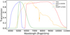 |
Fig. 1 Response curves for all the instruments in this paper, normalized at their peak transmission wavelength. |
2.2 TESS
TESS (Ricker et al. 2015) is an MIT-led NASA mission to search for transiting exoplanets around bright stars from the Galactic poles down to the Galactic plane. TESS has observed 26 segments of the sky with a 27.4-day observational period per segment (Ricker et al. 2015), making it sensitive to exoplanets with orbital periods shorter than 13 days. While observing a segment, TESS returns full frame images in a photometric bandpass between 600 and 1000 nm, similar to the Cousins I band, at a 30 min cadence. For stars with TESS magnitude 9–15, precisions on the order of 50 parts per million are attained. J1407 was observed by TESS in Sector 11 from 22 April 2019 to 21 May 2019. The TESS light curves of J1407 were extracted from the MAST archive using the eleanor (Feinstein et al. 2019) software package. The data for J1407 contain 744 observations over 23 days (a few days are missing due to light scattered from Earth that contaminated the data), and the resultant light curve is shown in Fig. 3. The standard deviation is about 0.014 for the normalized flux (equivalent to the transit depth of an object with radius 1.1 RJup for this specific star).
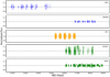 |
Fig. 2 Light curves for the five ground-based telescopes after correcting for both a downward linear trend and the dominant periodicitiesas described in Sect. 3.2. The lowest and highest 5% of the flux values for each separate telescope were removed. |
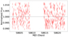 |
Fig. 3 Light curve of the TESS data after removing the dominant periodicities via the routine described in Sect. 3.2. The lowest and highest 5% of the flux values were removed. |
3 Analysis
3.1 Removal of long-term trends
In order to obtain the best sensitivity for planetary transits, the light curve needed to be corrected for the star’s variability. First, a long-term linear trend was removed by fitting a linear function to the light curve1. The fit was applied and removed for each of the ground-based data sets separately. The nature of this long-term trend will be discussed in more detail in a separate paper (Barmentloo et al., in prep.), but we note that the effect occurs in the ROAD, ASAS, and ASAS-SN data sets but not in the KELT or PROMPT data. The effect occurs most strongly (both in terms of gradient and signal-to-noise ratio) in the ROAD data, where it has a gradient of − 1.06 ± 0.02% per year from 2012 up to 2020. The gradient seen in the ASAS data set, which covers 2001 up to 2009 and is therefore independent from the ROAD data set, is similar at −1.07 ± 0.12% per year. A search in the ASAS data for stars around J1407 found a similar trend in a non-negligible number of stars, with preferentially negative gradients distributed around an average of about − 1% per year. Searching for the trend in ASAS in an equally sized area in a random part of the sky found no such trend at all, which suggests that this effect is of astrophysical origin.
3.2 Removing the rotational modulation
To further increase the sensitivity of the transit least squares (TLS) search (see Sect. 3.3), strong periodic signals in the light curve should be suppressed. To this end, each separate ground-based telescope data set was divided into segments. A new segment was started either when there was a 10 day gap between photometric points or when the segment would be longer than 500 days. For each of these segments, a Lomb–Scargle (LS) periodogram was calculated. The peak signal (most often the 3.2 day signal, but sometimes with another periodicity) was noted. Next, the segment was time-folded over the periodicity of exactly this peak signal, and to this a superposition of sines and cosines with different frequencies was fitted via the formula:
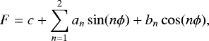 (1)
(1)
where F is the fitted flux, an and bn are the best-fit amplitudes, and c is the best-fit offset. The best-fit curve was then subtracted from the time-folded flux in each segment. As most segments still had a relatively strong periodic signal remaining, the process of determining the dominant segment signal and removing a best-fit curve was performed twice for each segment. The substantial decrease in power of periodic signals caused by this routine is shown for each telescope in Fig. 4. Finally, the now doubly corrected segments were recombined and the lowest and highest 5% of the flux values (i.e., a total of 10% of the flux values) were removed for each separate telescope. We removed these outliers as they, due to their depth, could not possibly have been part of a transit. The TLS algorithm would, however, try to take these outliers into account when fitting a transit, potentially causing it to miss injected transits. The light curves of the five separate telescopes were combined into one after the above routine was performed. The resulting light curve is shown in Fig. 2.
For the TESS data the same approach was used, with the only difference being the segment length: As the TESS data only span 25 days, the entire data set was considered as a single segment. Again, the routine was performed twice to remove signals less dominant than the 3.2 day signal. The resulting change in periodogram can be seen in Fig. 5.
We looked for long-term variations in the ~3.2 day signal in the ground-based data. The light curves from each ground-based telescope (in the form that they have after the correction in Sect. 3.1, but before the corrections in Sect. 3.2) were individually divided intosegments of data at points where there were large gaps in the observations. These segments were then divided into segments of 75-day durations, which we determined was the optimal value for minimizing the determined rotational period error (for a shorter segment size) and preventing the under-sampling of the activity cycle (for longer segment durations). If the segment itself spanned less than 75 days, it was simply considered as one segment. For a segment to be considered, there were two further requirements: Firstly, the segment had to have an average sampling of at least 2.5 data points per 3.2 days to adhere to the Nyquist sampling theorem (this criterion was never met by ASAS or ASAS-SN). Secondly, we required the LS periodogram from 2 to 5 days to have its peak value between 3.1 and 3.3 days to avoid sampling a segment with a dominant period other than the 3.2period. An LS periodogram was then calculated on each valid segment, and the highest peak in the periodogram between 3.1 and 3.3 days was taken to be the mean spot rotational period during the midpoint in time t of that segment, called Prot(t). The errors were determined using a bootstrap technique by generating data with the same cadence and standard deviation as the specific segment and adding to this a sine with a typical amplitude and a 3.2-day periodicity. The retrieved periodicities from multiple runs of the LS periodogram thus formed a Gaussian distribution, of which the standard deviation was taken to be the error on the determined period for that segment. These measured periods are shown in Fig. 6 and tabulated in Table 2.
The Python package emcee (Foreman-Mackey et al. 2013) was used to determine the activity cycle period by fitting a model to the data. Leaving out unknown asymmetries in the stellar activity, the activity cycle is periodic and on average well described by a sinusoid (Willamo et al. 2020). We modeled the activity cycle, Pactivity, as:
![Mathematical equation: \[ P_{\textrm{rot}}(t) = P_{\textrm{meanrot}}+a\sin (2\pi t/P_{\textrm{activity}}+\phi), \]](/articles/aa/full_html/2021/08/aa40768-21/aa40768-21-eq2.png)
where Pmeanrot is the mean spot rotational period, a is the amplitude of the variation in the spot rotational period, and ϕ determines the phase of the sinusoidal fit. An initial fit was carried out by the lmfit (Newville et al. 2014) package in Python, and then these values of Pmeanrot, a, Pactivity, and ϕ were used as initialization points for the walkers in the emcee routine.
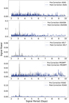 |
Fig. 4 Comparison of the LS periodograms before and after applying the routine from Sect. 3.2 for each of the ground-based telescopes. |
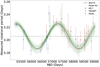 |
Fig. 6 Fitting of the long-term activity of J1407. The brown-red curve indicates the best fitting sinusoid. The dotted black line shows the (weighted) average rotation period. |
3.3 TLS search for transits
An optimized detection algorithm to search for transits is the TLS algorithm (Hippke & Heller 2019), which improves on the classical boxleast squares transit searching algorithm (Kovács et al. 2002). The TLS algorithm computes the signal detection efficiency (SDE) of each signal, which can be used to determine the uncertainty on the detection or to constrain the parameters that the given data would be sensitive to. For TLS, the SDE threshold for a false positive rate of 1% in simulated white noise data is SDE = 7. There is discussion as to what SDE value should be considered a confirmed transit. In the literature (Hippke & Heller 2019), detection thresholds from SDE = 6 to SDE = 10 can be found. During the transit-injection retrieval experiment described below, we adopted a detection threshold value of 6, as we know the orbital parameters of the injected transits a priori. We inserted artificial transits into the ground-based telescope data and determined the retrieval fraction for different values of the orbital period and planetary radius. For the creation of fake transit signals, the BATMAN package (Kreidberg 2015) was used. The parameters used for the star and for the exoplanet’s orbit are given in Table 3. For the transits created by BATMAN, a nonlinear, four-parameter limb darkening model was used with the specific limb darkening coefficients for J1407 approximated as a Teff = 4500 K, log (g) = 4.0 m s−2 surface gravity star, and the corresponding values from Claret & Bloemen (2011) were used.
The planetary radius was varied in steps of 0.15 RJup from 0.5 up to 2.0 RJup. The orbital period was varied in 100 logarithmically spaced steps from 3 to 40 days. For every combination of planetary radius and orbital period, ten trial runs were done. For each trial an arbitrary time of inferior conjunction (offset) between 0 and the inserted orbital period was chosen from a uniform distribution. This process was performed twice: once with artificial transits inserted into the activity-removed light curve and once with the transits inserted in an artificial light curve that included white (Gaussian) noise, with identical observation times and flux errors as the real data but with randomized flux values.
Parameters for the injected transits.
4 Results
4.1 Characterization of the rotation period variability
The exact periodicity of starspots varies over a timescale of years, which we attribute to starspots migrating to and from the equator. Due to the differential rotation of the star, there are different rotational periods at each latitude, analogous to the 11 yr Schwabe cycle of the Sun (Hathaway 2015). In Fig. 6, after removing best-fit period values at the edge of the period grid (less than 3.1 or greater than 3.3 days, indicating a failed fit), the most likely periods were plotted at the midpoints of the intervals used for the calculation and color-coded for the respective source. A sinusoidalpattern is visible in Fig. 6. Further confirmation is provided when determining the difference inthe Bayesian information criterion (BIC) between a linear fit and the best sine fit. We determined the BIC values using the weighted least squares version of the Gaussian case. Despite the penalty of having four free parameters compared to the two free parameters for a linear fit, the BIC value for the sine fit is about 32 times lower than that for a linear fit (9 and 41, respectively). This delta BIC confirms the perceived sinusoidal pattern.
The best fitting value for the period cycle of J1407 is found to be 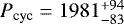 days, where the calculated rotation period oscillates around the median, Prot = 3.206 ± 0.002 days, with an amplitude, a, of 0.020 ± 0.003 days. We note that the logarithm of the ratio of the periods is logProt∕Pcyc = −2.79 and that this is at least consistent with other young K-type stars (Saar & Brandenburg 1999). J1407 is a young star and has X-ray emission consistent with saturation (log LX∕LBOL = −3.4; Mamajek et al. 2012), which is typically seen around − 3.2 ± 0.2, and this is expected for rotation periods of less than about 3.5 days for K5 stars (Pizzolato et al. 2003). The star is therefore in a regime where the magnetic activity is no longer following the dynamo model relation, and so interpreting the periodic variation in the rotational period in terms of the dynamo model of magnetic activity should be done with caution.
4.2 Transit search
A TLS planet search was performed on the data from Fig. 2. Values between 3 and 40 days for the orbital period were considered. The resulting SDE spectrum is given in the upper panel of Fig. 7 and shows no significant periodicities. The highest TLS value is found to be 9.09, at an orbital period of 8.03 days, which is above our detection threshold value of 6. In the lower panel of Fig. 7 the fitted model to this 8.03 day signal is not a convincing transit, the signal most likely being a remnant of the often integer day observation cadences.
A TLS search was performed on the TESS light curve over an orbital period grid from 1.5 to 6 days. This yielded a TLS spectrum with lower powers, the maximum SDE value reached being just over 4. As such, no significant periodicities are present in the TESSdata.
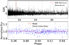 |
Fig. 7 Upper plot: transit least squares (TLS) spectrum for the ground-based data. The TLS maximum has a value of 9.09 and is located at an orbital period of 8.03 days. Lower plot: ground-based data folded over the most likely orbital period. The fitted model for the transit has a depth of 1.4% (1.1 RJup) and a duration of 0.093 days. |
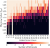 |
Fig. 8 Sensitivity of the TLS algorithm in the J1407 system for generated transits with different radii and orbital periods injected in the real data. Columns on the right-hand side of the plot are broader than ones on the left-hand side due to the logarithmic grid spacing. The corresponding masses were taken from the 20 Myr AMES-Dusty models (Allard et al. 2001). |
4.3 TLS sensitivity
The final results of the procedure described in Sect. 3.3 can be seen in Fig. 8 for the real data and in Fig. 9 for the generated data. Both figures show a similar pattern, with transits of shorter orbital period and larger planetary radius being retrieved more often. The vertical lines in Fig. 8 with higher retrieval rates than their surroundings are most likely caused by residual low power periodic signals in the data, which are just barely able to pass our SDE threshold. When a planet with a similar periodicity to these remaining signals is injected, the algorithm then detects the remaining signal instead of the transit, seemingly always recovering the planet independent of radius. These lines should therefore beinterpreted as an artifact of the methodology, and not as the periodicities to which we are more sensitive. The real retrieval rates for these periodicities are best estimated as being equal to their surrounding periodicities.
Another clear trend is that the critical radius at which transits start to be retrieved is systematically smaller for the generated data. This is due to the simulated data being generated with ideal Gaussian noise, while the real data have additional red noise due to the atmosphere and un-modeled systematic effects.
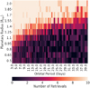 |
Fig. 9 Sensitivity of the TLS algorithm for injected planets where the photometry is generated with white noise and with the same observing epochs as the J1407 data. The corresponding masses were estimated using the 20 Myr AMES-Dusty models (Allard et al. 2001). |
5 Discussion
No additional transiting objects were found in the J1407 system. Upper limits on the radii of potentially missed planets were determined for different orbital periods: For a 3 day orbital period, the 50% injected planet recovery fraction radius is 0.95 RJup; for 10 days it is 1.25 RJup; and for 20 days it is no larger than 1.4 RJup. As the system is still very young, any Jupiter-mass planet on a short orbit would also be young and hot, inflating potential planets to well above the detectable radius limits placed by our analysis. Our TLS analysis therefore rules out planetary mass companions at shorter orbital periods.
The planetary occurrence rate for G-type stars (the type J1407 will be once it reaches the main sequence) on our tested orbital period and radius grid is below 1% (Kunimoto & Matthews 2020). The sensitivity plots (Figs. 8 and 9) show similar trends as the ones used in the search for planets orbiting β Pictoris in Lous et al. (2018), where they exclude a Jupiter-sized planet (in terms of both mass and radius) at the shortest orbital periods.
Ma & Ge (2014) argue that two distinct brown dwarf (BD) formation mechanisms exist; BDs with masses below 42.5 MJup are thought to be formed from a protoplanetary disk, while BDs with masses above 42.5 MJup would form more like stellar binaries. With a mass of 60–100 MJup, J1407 b should be firmly in the latter group, although a large orbital period could potentially put the mass of J1407 b around the lower limit of 20 MJup (Kenworthy et al. 2015). Combined with the presumed high eccentricity of J1407 b (derived from the large measured transverse velocity and lack of eclipse detected for a circular orbit, as discussed in Kenworthy et al. 2015), the absence of greater than Jupiter-sized planets in the inner part of the system is another hint that J1407 was indeed formed more like a binary without the presence of any protoplanetary disk.
6 Conclusions
We modeled and removed the dominant periodic component from the light curve of the star J1407, performed a search for transits of substellar companions, and examined the light curve for any other anomalous features. We detected and characterized the rotational period cycle for J1407, which was found to be consistent for a young K-type star, using data from several ground-based telescopes with a combined baseline of 19 yr. After removing a simple model for the stellar activity, we searched the activity subtracted data, as well as 25 days of short cadence TESS data, for exoplanet transits. No plausible transit signal was found, allowing us to constrain the presence of transiting planets within the sampled period-radius space to companions no larger than about 1.25 RJup and with periods of less than 40 days. Further monitoring of the J1407 system continues, in anticipation of the next eclipse of J1407b.
Acknowledgements
We thank the referee for a careful reading of our manuscript – their suggestions have improved the paper. This research has used the SIMBAD database, operated at CDS, Strasbourg, France (Wenger et al. 2000). This work has used data from the European Space Agency (ESA) mission Gaia (https://www.cosmos.esa.int/gaia), processed by the Gaia Data Processing and Analysis Consortium (DPAC, https://www.cosmos.esa.int/web/gaia/dpac/consortium). Funding for the DPAC has been provided by national institutions, in particular the institutions participating in the Gaia Multilateral Agreement. To achieve the scientific results presented in this article we made use of the Python programming language (Python Software Foundation, https://www.python.org/), especially the SciPy (Virtanen et al. 2020), NumPy (Oliphant 2006), Matplotlib (Hunter 2007), emcee (Foreman-Mackey et al. 2013), and astropy (Astropy Collaboration 2013, 2018) packages. We acknowledge with thanks the variable star observations from the AAVSO International Database contributed by observers worldwide and used in this research. We thank the Las Cumbres Observatory and its staff for its continuing support of the ASAS-SN project. We also thank the Ohio State University College of Arts and Sciences Technology Services for helping us set up and maintain the ASAS-SN variable stars and photometry databases. ASAS-SN is supported by the Gordon and Betty Moore Foundation through grant GBMF5490 to the Ohio State University and NSF grant AST-1515927. Development of ASAS-SN has been supported by NSF grant AST-0908816, the Mt. Cuba Astronomical Foundation, the Center for Cosmology and AstroParticle Physics at the Ohio State University, the Chinese Academy of Sciences South America Center for Astronomy (CASSACA), the Villum Foundation, and George Skestos. Early work on KELT-North was supported by NASA Grant NNG04GO70G. Work on KELT-North was partially supported by NSF CAREER Grant AST-1056524 to S. Gaudi. Work on KELT-North received support from the Vanderbilt Office of the Provost through the Vanderbilt Initiative in Data-intensive Astrophysics. Part of this research was carried out in part at the Jet Propulsion Laboratory, California Institute of Technology, under a contract with the National Aeronautics and Space Administration (80NM0018D0004).
References
- Allard, F., Hauschildt, P. H., Alexander, D. R., Tamanai, A., & Schweitzer, A. 2001, ApJ, 556, 357 [NASA ADS] [CrossRef] [Google Scholar]
- Astropy Collaboration (Robitaille, T. P., et al.) 2013, A&A, 558, A33 [NASA ADS] [CrossRef] [EDP Sciences] [Google Scholar]
- Astropy Collaboration (Price-Whelan, A. M., et al.) 2018, AJ, 156, 123 [Google Scholar]
- Braga-Ribas, F., Sicardy, B., Ortiz, J. L., et al. 2014, Nature, 508, 72 [NASA ADS] [CrossRef] [Google Scholar]
- Charnoz, S., Crida, A., & Hyodo, R. 2018, Rings in the Solar System: A Short Review (Springer International Publishing AG), 54 [Google Scholar]
- Claret, A., & Bloemen, S. 2011, VizieR Online Data Catalog, J/A+A/529/A75 [Google Scholar]
- Feinstein, A. D., Montet, B. T., Foreman-Mackey, D., et al. 2019, PASP, 131, 094502 [Google Scholar]
- Foreman-Mackey, D., Hogg, D. W., Lang, D., & Goodman, J. 2013, PASP, 125, 306 [Google Scholar]
- Guinan, E. F., & Dewarf, L. E. 2002, ASP Conf. Ser., 279, Toward Solving the Mysteries of the Exotic Eclipsing Binary ∈ Aurigae: Two Thousand years of Observations and Future Possibilities (PASP), 121 [Google Scholar]
- Hambsch, F. J. 2012, J. Am. Assoc. Variable Star Observers (JAAVSO), 40, 1003 [NASA ADS] [Google Scholar]
- Hathaway, D. H. 2015, Liv. Rev. Solar Phys., 12, 4 [NASA ADS] [CrossRef] [Google Scholar]
- Hippke, M., & Heller, R. 2019, A&A, 623, A39 [NASA ADS] [CrossRef] [EDP Sciences] [Google Scholar]
- Hunter, J. D. 2007, Comput. Sci. Eng., 9, 90 [NASA ADS] [CrossRef] [Google Scholar]
- Kenworthy, M. A., & Mamajek, E. E. 2015, AJ, 800, 126 [NASA ADS] [CrossRef] [Google Scholar]
- Kenworthy, M. A., Lacour, S., Kraus, A., et al. 2015, MNRAS, 446, 411 [NASA ADS] [CrossRef] [Google Scholar]
- Kochanek, C. S., Shappee, B. J., Stanek, K. Z., et al. 2017, PASP, 129, 104502 [Google Scholar]
- Kovács, G., Zucker, S., & Mazeh, T. 2002, A&A, 391, 369 [NASA ADS] [CrossRef] [EDP Sciences] [Google Scholar]
- Kreidberg, L. 2015, PASP, 127, 1161 [NASA ADS] [CrossRef] [Google Scholar]
- Kunimoto, M., & Matthews, J. M. 2020, AJ, 159, 248 [NASA ADS] [CrossRef] [Google Scholar]
- Lipunov, V., Gorbovskoy, E., Afanasiev, V., et al. 2016, A&A, 588, A90 [NASA ADS] [CrossRef] [EDP Sciences] [Google Scholar]
- Lous, M. M., Weenk, E., Kenworthy, M. A., Zwintz, K., & Kuschnig, R. 2018, A&A, 615, A145 [NASA ADS] [CrossRef] [EDP Sciences] [Google Scholar]
- Ma, B., & Ge, J. 2014, MNRAS, 439, 2781 [NASA ADS] [CrossRef] [Google Scholar]
- Mamajek, E. E., Quillen, A. C., Pecaut, M. J., et al. 2012, AJ, 143, 72 [Google Scholar]
- Mentel, R. T., Kenworthy, M. A., Cameron, D. A., et al. 2018, A&A, 619, A157 [NASA ADS] [CrossRef] [EDP Sciences] [Google Scholar]
- Mikolajewski, M., & Graczyk, D. 1999, MNRAS, 303, 521 [NASA ADS] [CrossRef] [Google Scholar]
- Newville, M., Stensitzki, T., Allen, D. B., & Ingargiola, A. 2014, LMFIT: Non-Linear Least-Square Minimization and Curve-Fitting for Python [Google Scholar]
- Oliphant, T. E. 2006, A Guide to NumPy, vol. 1 (Trelgol Publishing USA) [Google Scholar]
- Pepper, J., Pogge, R. W., DePoy, D. L., et al. 2007, PASP, 119, 923 [NASA ADS] [CrossRef] [Google Scholar]
- Pepper, J., Kuhn, R. B., Siverd, R., James, D., & Stassun, K. 2012, PASP, 124, 230 [Google Scholar]
- Pizzolato, N., Maggio, A., Micela, G., Sciortino, S., & Ventura, P. 2003, A&A, 397, 147 [NASA ADS] [CrossRef] [EDP Sciences] [Google Scholar]
- Pojmanski, G. 1997, Acta Astron., 47, 467 [Google Scholar]
- Reichart, D., Nysewander, M., Moran, J., et al. 2005, Nuovo Cimento C Geophys. Space Phys. C, 28, 767 [Google Scholar]
- Ricker, G. R., Winn, J. N., Vanderspek, R., et al. 2015, J. Astron. Telescopes Instrum. Syst., 1, 014003 [Google Scholar]
- Rieder, S., & Kenworthy, M. A. 2016, A&A, 596, A9 [NASA ADS] [CrossRef] [EDP Sciences] [Google Scholar]
- Rodriguez, J. E., Stassun, K. G., Lund, M. B., et al. 2016, AJ, 151, 123 [CrossRef] [Google Scholar]
- Saar, S. H., & Brandenburg, A. 1999, ApJ, 524, 295 [NASA ADS] [CrossRef] [Google Scholar]
- Tiscareno, M. S. 2013, Planetary Rings (Dordrecht: Springer Science+Business Media), 309 [Google Scholar]
- Virtanen, P., Gommers, R., Oliphant, T. E., et al. 2020, Nat. Methods, 17, 261 [Google Scholar]
- Wenger, M., Ochsenbein, F., Egret, D., et al. 2000, A&AS, 143, 9 [NASA ADS] [CrossRef] [EDP Sciences] [Google Scholar]
- Willamo, T., Hackman, T., Lehtinen, J. J., et al. 2020, A&A, 638, A69 [NASA ADS] [CrossRef] [EDP Sciences] [Google Scholar]
- Zanazzi, J. J., & Lai, D. 2017, MNRAS, 464, 3945 [NASA ADS] [CrossRef] [Google Scholar]
The entire code used for the analysis and for creating the figures in this paper is available at https://github.com/StanBarmentloo/J1407_transit_search_activity
All Tables
All Figures
|
Fig. 1 Response curves for all the instruments in this paper, normalized at their peak transmission wavelength. |
| In the text | |
|
Fig. 2 Light curves for the five ground-based telescopes after correcting for both a downward linear trend and the dominant periodicitiesas described in Sect. 3.2. The lowest and highest 5% of the flux values for each separate telescope were removed. |
| In the text | |
|
Fig. 3 Light curve of the TESS data after removing the dominant periodicities via the routine described in Sect. 3.2. The lowest and highest 5% of the flux values were removed. |
| In the text | |
|
Fig. 4 Comparison of the LS periodograms before and after applying the routine from Sect. 3.2 for each of the ground-based telescopes. |
| In the text | |
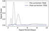 |
Fig. 5 Same as Fig. 4, but for the TESS data. |
| In the text | |
|
Fig. 6 Fitting of the long-term activity of J1407. The brown-red curve indicates the best fitting sinusoid. The dotted black line shows the (weighted) average rotation period. |
| In the text | |
|
Fig. 7 Upper plot: transit least squares (TLS) spectrum for the ground-based data. The TLS maximum has a value of 9.09 and is located at an orbital period of 8.03 days. Lower plot: ground-based data folded over the most likely orbital period. The fitted model for the transit has a depth of 1.4% (1.1 RJup) and a duration of 0.093 days. |
| In the text | |
|
Fig. 8 Sensitivity of the TLS algorithm in the J1407 system for generated transits with different radii and orbital periods injected in the real data. Columns on the right-hand side of the plot are broader than ones on the left-hand side due to the logarithmic grid spacing. The corresponding masses were taken from the 20 Myr AMES-Dusty models (Allard et al. 2001). |
| In the text | |
|
Fig. 9 Sensitivity of the TLS algorithm for injected planets where the photometry is generated with white noise and with the same observing epochs as the J1407 data. The corresponding masses were estimated using the 20 Myr AMES-Dusty models (Allard et al. 2001). |
| In the text | |
Current usage metrics show cumulative count of Article Views (full-text article views including HTML views, PDF and ePub downloads, according to the available data) and Abstracts Views on Vision4Press platform.
Data correspond to usage on the plateform after 2015. The current usage metrics is available 48-96 hours after online publication and is updated daily on week days.
Initial download of the metrics may take a while.