| Issue |
A&A
Volume 652, August 2021
|
|
|---|---|---|
| Article Number | A79 | |
| Number of page(s) | 8 | |
| Section | The Sun and the Heliosphere | |
| DOI | https://doi.org/10.1051/0004-6361/202140656 | |
| Published online | 13 August 2021 | |
Reconstructing solar magnetic fields from historical observations
VII. Far-side activity in surface flux transport simulations
1
Space physics and astronomy research unit, University of Oulu, PO Box 3000, 90014 Oulu, Finland
e-mail: This email address is being protected from spambots. You need JavaScript enabled to view it.
2
National Solar Observatory, Boulder, CO 80303, USA
Received:
25
February
2021
Accepted:
2
May
2021
Abstract
Context. The evolution of the photospheric magnetic field can be simulated with surface flux transport (SFT) simulations, which allow for the study of the evolution of the entire field, including polar fields, solely using observations of the active regions. However, because only one side of the Sun is visible at a time, active regions that emerge and decay on the far-side are not observed and not included in the simulations. As a result, some flux is missed.
Aims. We construct additional active regions and apply them to the far-side of the Sun in an SFT simulation to assess the possible effects and the magnitude of error that the missing far-side flux causes. We estimate how taking the missing far-side flux into account affects long-term SFT simulations.
Methods. We identified active regions from synoptic maps of the photospheric magnetic field between 1975 and 2019. We divided them into solar cycle wings and determined their lifetimes. Using the properties of observed active regions with sufficiently short lifetimes, we constructed additional active regions and inserted them into an SFT simulation.
Results. We find that adding active regions with short lifetimes to the far-side of the Sun results in significantly stronger polar fields in minimum times and slightly delayed polarity reversals. These results partly remedy the earlier results, which show overly weak polar fields and polarity reversals that are slightly too early when far-side emergence is not taken into account. The far-side active regions do not significantly affect poleward flux surges, which are mostly caused by larger long-living active regions. The far-side emergence leads to a weak continuous flow of flux, which affects polar fields over long periods of time.
Key words: Sun: photosphere / Sun: magnetic fields / Sun: activity
© ESO 2021
1. Introduction
The photospheric magnetic field is an important driver of space weather and knowledge of its nature is needed to understand and predict, for example, certain properties of solar wind and solar eruptions, such as flares and coronal mass ejections. These phenomena and their interaction with the magnetic field of the Earth, which produces geomagnetic activity, make the photospheric magnetic field a very important topic of research.
Daily magnetographic observations of the photospheric magnetic field have been continuously underway since the early 1970s (Howard 1974; Livingston et al. 1976). Stanford University began providing daily low-resolution full-disk maps in 1976. Observations have continued at the Wilcox Solar Observatory (WSO), which is operated by the university (Scherrer et al. 1977). Multiple other observatories, such as the National Solar Observatory at Kitt Peak and the Mount Wilson observatory, have also maintained instruments over many decades and provided extended continuous series of observations at higher resolutions (for a review of early full-disk magnetographic observations see Pevtsov et al. 2021). Subsequently, space-based instruments, such as the SOHO/MDI and SDO/HMI have been launched, providing observations that can be compiled together with those of the ground-based instruments. Space-based instruments have the advantage that they are not affected by the effects of the Earth’s atmhosphere.
However, one shortcoming of all ground-based instruments and most space-based instruments is that they observe only the side of the Sun that is visible from the Earth. It is possible to fly spacecraft into orbits that also reveal the so-called far-side of the Sun, but few such missions have been launched. None of the past missions that observed the Sun at different vantage points had a magnetograph on board. All the instruments that have provided continuous observations of magnetic fields for long periods of time have been either on the ground or in orbit near the Earth.
Since the Sun is in rotation, the long-lived features that emerge on the far-side are eventually seen on the near-side that is facing the Earth. However, the short-lived features that emerge and disappear on the far-side before rotating into Earth’s view are not observed from the Earth at all. One of the features that can potentially be missed are small active regions, which typically have lifetimes ranging from days to weeks. While short-lived active regions may well emerge and disappear without being seen from the Earth, the magnetic flux contained within them could still have a cumulative effect on the large-scale photospheric magnetic field.
A surface flux transport model is a tool that can be used to study the evolution of the photospheric magnetic field. It takes as its input the new flux emerging in active regions, which can be reconstructed from sunspot areas (Jiang et al. 2010; Baumann et al. 2004) or numbers (Jiang et al. 2011) or directly assimilated from magnetograms (Yeates et al. 2015; Virtanen et al. 2017, 2018; Whitbread et al. 2017). An SFT model simulates the transport and decay of the active regions to generate a full map of the photospheric magnetic field. Since the input is typically based on observations of only the near-side of the Sun, the active regions on the far-side that were missed are not included, and their absence could affect the simulation and the total amount of flux.
In this paper, we study the lifetimes of active regions and the effect that hidden far-side active regions could have in an SFT simulation. We determine the lifetimes of active regions in an SFT simulation and compare them with observed lifetimes. Based on the lifetimes and other statistical properties of the observed active regions, we create additional active regions that are used as approximations of the real active regions that could be hidden on the far-side of the Sun. We then insert the additional far-side active regions into an SFT simulation along with the observed active regions and study the effects they have on the simulated large-scale photospheric magnetic field.
The paper is structured as follows. In Sect. 2, we present the data used in this study. In Sect. 3, we review the active region identification process and the details of the SFT model. In Sect. 4, we compute the simulated and observed lifetimes of active regions. In Sect. 5, we show the construction method for additional active regions. In Sect. 6, we present the results of simulations, and in Sect. 7 we give our conclusions.
2. Data
The line-of-sight photospheric magnetic field was observed at the NSO at Kitt Peak from February 1975 until March 1992 with a 512-channel diode array magnetograph (Livingston et al. 1976), and thereafter with a CCD spectromagnetograph until August 2003 (Jones et al. 1992). In August 2003, SOLIS/VSM started operation and replaced the earlier instrumentation (Keller et al. 2003). SOLIS ceased operating in October 2017, whereas SDO/HMI has been operating since April 2010. A brief review of magnetographic measurements of solar magnetic fields can be found in Pevtsov et al. (2021). In this work we used NSO/SOLIS and HMI synoptic maps, as well SOLIS full-disk magnetograms. NSO/SOLIS (a combined data set including early NSO magnetographs and SOLIS/VSM) synoptic maps were used from the beginning of cycle 21 in late 1975 until October 2017, and thereafter HMI synoptic maps were used until April 2019. There are seven rotations missing from the SOLIS data between April 2010 and October 2017, including a gap of four rotations in the summer of 2014 (Carrington rotations (CR) 2152–2155), when SOLIS was relocated. These missing rotations were filled with HMI data. Missing rotations in NSO/SOLIS data before April 2010 were not filled, which means that a total of 19 rotations are missing from the final data set, out of the 591 in the studied time period. It should also be noted that not all of the included synoptic maps are complete. If during a rotation a certain Carrington longitude was not observed near the central meridian due to a gap in observations, observations from nearer the limb were used instead. This can lead to artifacts and distortion in the synoptic map, and sometimes narrow longitude bands seem to be missing completely and have been filled with zeros. However, the data coverage is generally good as evidenced by the relatively low number of missing complete rotations. The resolution of the maps (number of pixels covering ±90 degrees in latitude and 0–360 degrees in longitude) is 180 × 360 pixels. The grid is evenly spaced in longitude and sine of latitude. The NSO/SOLIS maps were published in this format by the instrument teams. The resolution of the original HMI maps is 1440 × 3600, but we reduced the resolution to the same 180 × 360 by averaging. This eliminates problems which could arise from the different spatial resolutions of the instruments. Pietarila et al. (2013) has shown that flux densities in spatially smoothed SDO/HMI data and SOLIS/VSM data are in good agreement. The SOLIS full-disk data usually contains at least one image per day, although sometimes several observations were taken on the same day. Observation times also vary from day to day by a few hours.
The data have not been scaled, so the replacement of KP by SOLIS in 2003, and then the switch from SOLIS to HMI in 2017 may affect field intensity values. Scaling between KP and SOLIS is difficult, because the two data sets do not overlap. The scaling coefficient between HMI and SOLIS is fairly close to one (Pietarila et al. 2013; Riley et al. 2014; Virtanen & Mursula 2017). The end of SOLIS period is in the late declining phase of cycle 24, when activity is already very low. Only about 10% of all active regions in cycle 24, including those during SOLIS data gaps, are identified from HMI maps. This is why the scaling between SOLIS and HMI still has a negligible effect. In this article we mainly study the differences between the different simulations, which are all affected by the same changes in the data source. Good data coverage is, in this case, more important than small differences in magnetic field intensity between the different data sets.
3. Active region identification and SFT model
We identified active regions from each synoptic map of the data set with the method presented in Virtanen et al. (2018). The sum of the signed flux of each synoptic map, that is, the flux imbalance, was first removed by subtracting the mean value from every pixel of the map. The maps were then connected to make one large map spanning the time frame from the first observation in the data set to the last. This helped us in identifying active regions in cases where the region was partly located on one synoptic map and partly on another. The large map was then transformed to an absolute value map and smoothed with a Gaussian filter. The width of the filter was four pixels in both latitude and longitude and the standard deviation was two pixels. The filter was applied to remove small gaps, or drops in field intensity, which might otherwise divide the active region into multiple separate regions that would be identified as multiple, typically highly unbalanced, active regions.
We then applied a threshold of 50G to each pixel value and defined all connected groups of pixels above the threshold to be active regions; by connected we mean that the sides or corners of two pixels touch. The identified regions were then selected from the original unsmoothed map pixel by pixel. The flux imbalance was removed from each active region by subtracting the active region mean value from every pixel inside the region. The flux balancing is required to prevent unphysical monopole components from forming. The trailing polarity part of an active region tends to be weaker and more spread out than the leading polarity part, resulting in more leading polarity flux being selected when active regions are identified. If the total imbalance of the region was more than half of the total unsigned flux inside it, meaning that if total flux of the weaker polarity was less than one third of the stronger, the region was discarded. All emerging active regions should be roughly flux-balanced, so a very large flux imbalance suggests an erroneously identified active region. The average unsigned imbalance of an active region is about 16% of the total flux of the region, and the average absolute correction is about 16G. The distribution of the corrections is close to normal with zero mean, so most active regions only receive relatively small corrections. The flux-balanced active regions have been shown to work well in SFT simulations and produce simulated magnetic fields that agree with the observations (Yeates et al. 2015; Virtanen et al. 2017).
Once the active regions were identified, we divided them into separate solar cycle wings. A wing consists of all active regions emerging in one hemisphere during a solar cycle. Because the last active regions of the previous cycle may emerge at low latitudes at the same time as the first regions of the following cycle appear at higher latitudes, the wings may overlap in minimum times. In this paper, we study the wings of cycles 21–24. The last few active regions of cycle 20, which can be seen in the Kitt Peak maps, but do not belong to any of the studied wings, were discarded. The locations of the active regions are shown in Fig. 1. Wings have been marked with different colors to make them easier to separate.
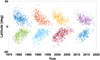 |
Fig. 1. Latitude and observation time of identified active regions. Different solar cycle wings have been marked with different colors for clarity. |
The SFT model used in this work has previously been used and tested in several other studies (Yeates et al. 2015; Virtanen et al. 2017, 2018). We include here only a short description of the model. For a more detailed description, testing, and validation of the model, see Yeates et al. (2015) and Virtanen et al. (2017).
The radial magnetic field Br(θ, ϕ, t) is written in the spherical coordinate system in terms of the two-component vector potential [Aθ, Aϕ]:
 (1)
(1)
where R is the radius of the Sun, θ is colatitude, ϕ is the azimuth angle, and t is time. The vector potential evolves over time, as follows
 (2)
(2)
 (3)
(3)
where ω(θ) is the differential angular velocity of rotation, D is the supergranular diffusivity coefficient, and uθ(θ) is the velocity of meridional circulation. Sθ and Sϕ represent the emergence of new flux in active regions. We used active regions identified from synoptic maps with the method described above. The active regions were inserted into the simulated radial field when they cross the central meridian, each pixel replacing the corresponding pixel in the simulation. The flux imbalance of the area was preserved by calculating it before the insertion and applying the mean imbalance back to every pixel after the insertion.
The angular velocity of differential rotation in the Carrington frame ω(θ) is:
 (4)
(4)
and the latitudinal profile of the meridional circulation is:
 (5)
(5)
We used a supergranular diffusion coefficient of D = 400 km2 s−1 and a peak meridional circulation speed of u0 = 11 m s−1. A discussion of the optimization of parameters is presented in Virtanen et al. (2017) and Whitbread et al. (2017).
While the speeds of meridional circulation and differential rotation are in this study assumed to be constant, we acknowledge that several studies have shown that they may change in time (Beck et al. 2002; Ulrich & Boyden 2005; Ulrich 2010; Ulrich & Tran 2013). This may have some effect on the results of the simulations. However, Virtanen et al. (2017) demonstrated that the surface flux transport model is relatively insensitive to such variations.
The model also uses the decay term from Baumann et al. (2006). This term models the slow temporal decay of the radial field with the following equation:
 (6)
(6)
where E(θ, ϕ, t) is the decay rate, Ylm(θ, ϕ) are spherical harmonics, clm are the harmonic coefficients of the simulated radial field at time t and τl are the decay times for each harmonic mode l. Only low harmonic modes with decay times of more than one year are included, which is why the value of l does not go above l = 9 (see Table 1 in Virtanen et al. 2017).
4. Active region lifetime
We determined the simulated lifetime of each identified active region using the SFT model. We inserted each identified active region into the SFT simulation alone, meaning that the simulation was started from a synoptic map that contains one active region and is zero elsewhere. We then began running the simulation, but stopped it after simulating one hour and then ran the active region identification algorithm on the simulated magnetic field. This was repeated until the active region in the simulation was no longer identified as an active region. The simulation time it took to get to this point was defined to be the lifetime of the active region. It is an approximation of the time it takes for the observed active region to spread and decay until it can no longer be identified as an active region.
It should be noted that there are some uncertainties in this method. First of all, the observed active region may already have decayed for some time before it was observed or it might still be emerging, resulting in a shorter simulated lifetime. Since synoptic maps are constructed mainly from observations near the central meridian, we have only one snapshot from the evolution of each active region. Because emergence is a much faster process than decay, many more active regions are already decaying than are still emerging, and as a result, we are likely to, on average, underestimate lifetimes and overestimate the number of short-lived active regions. Second, the simulation itself is a simplified model of the decay of active regions and not perfectly accurate, especially on small scales. Also, since the evolution of only one active region is simulated at a time, interactions between active regions that may affect the lifetime of the regions are not taken into account.
To assess the accuracy of the simulated lifetimes, we used SOLIS full-disk magnetograms to determine the observed lifetimes of active regions. Similarly to the active region identification used with the synoptic maps, we applied a Gaussian smoothing filter and then a threshold of 50G to the full-disk images, and defined all connected pixels with intensities above the threshold as belonging to the same active region. We repeated this for all the daily full-disk magnetograms and compared the locations of active regions to follow their rotation. If at least 50% of the pixels of an active region were within an active region identified on the previous day, they were defined as being the same active region. If there was a data gap of more than two days, the tracking was stopped, and all active regions after the gap were identified as new. We determined the number of consecutive days during which the same active region was observed and we defined this as the observed lifetime of the active region. However, because the full-disk magnetograms show only the near-side of the Sun, the maximum tracking time is limited to the time it takes for an active region to rotate to the far-side. This means that the maximum observed lifetime of an active region is about half a rotation, or two weeks, while the maximum observed lifetime of an active region emerging on the near-side is even significantly less, depending on the longitude with respect to the central meridian at which it emerges. The simulated lifetimes, on the other hand, do not have an upper limit.
In addition to our characterization of the lifetimes of active regions, we also computed their total unsigned flux. In the case of the active regions identified from the synoptic maps, the flux at the moment of the only available observation was used. Due to the way synoptic maps are constructed from full-disk images, this observation is usually from near the central meridian. In the case of active regions identified and tracked from the full-disk images the observation with the maximum flux was used. This gives a better estimate of the flux after emergence, when the active region starts to decay. Because the simulation uses the central meridian flux of the synoptic map as the starting point when it computes the simulated lifetime, the central meridian flux is also effectively the maximum flux in the simulation. This is why the maximum flux of the full-disk images is used here instead of the central meridian flux. It should be noted that due to the effect of the viewing angle, the values in the full-disk images are less accurate near the limb, resulting in larger uncertainties in the total fluxes.
Figure 2 shows the simulated and observed lifetimes of active regions as a function of their total unsigned flux. The simulated lifetimes clearly show that in order to reach a certain lifetime, an active region must contain a certain minimum amount of flux. However, a certain amount of flux does not guarantee a certain lifetime. Even active regions with large amounts of flux can in some cases have short lifetimes. This can be caused by a quicker separation of polarities, which causes the areas of different polarities to be detected as separate areas of intense magnetic field rather than as an active region, or faster than average cancellation of flux, which may happen in complicated structures containing both polarities and causes the field to quickly decay below the used threshold of 50G.
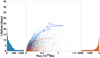 |
Fig. 2. Relationship between active region lifetime and total magnetic flux. Middle panel: simulated and observed lifetimes of active regions as functions of their total unsigned flux. Blue markers are simulated lifetimes obtained from SFT simulations using NSO/SOLIS and HMI synoptic maps. Red markers are observed lifetimes obtained from SOLIS full-disk magnetograms. The solid blue and red curves show the median flux in lifetime bins with a width of one day for simulated and observed lifetimes, respectively. The blue and red bars on the left and right show the number of active regions in each bin. |
The observed lifetimes show a fairly similar behaviour. The minimum flux required for a certain observed lifetime is generally slightly lower than for the simulated lifetimes. However, a fairly similar median curve can be observed, at least for the lifetime range covered by the observed lifetimes. The median flux of active regions tends to be slightly higher in the observed lifetimes than the simulated lifetimes.
5. Far-side active regions
To simulate active region emergence on the far-side of the Sun, we created additional active regions that were inserted to the SFT simulation on the far-side. The number of these additional active regions was determined by the number of observed active regions. We set a lifetime limit and, for each observed active region with a simulated lifetime below the limit, an additional active region was added. It should be noted that because in the construction of synoptic maps observations near the central meridian are weighted more heavily, not all active regions in the near-side are included in synoptic maps. If, for example, an active region emerges in an area that has already rotated over the central meridian, it may be included in the construction of the synoptic map, but the weight of the observation where the active region is present is smaller than the weight of earlier observations in which the same surface area was nearer the central meridian, but the active region was not present. As a result, in the final map the active region may be so faint that it remains below the 50G threshold and is not identified as an active region. On the other hand, if there are no observations of the area near the central meridian, or if the active region is strong enough, it can still reach the 50G threshold in the synoptic map and be identified as an active region.
Due to the facts discussed above, whether an active region is identified in the synoptic map depends not only on the properties of the active region itself but also on how many full-disk images the surface area of the active region are visible and where the active region was when those full-disk images were taken. Consequently, it is not possible to set an exact limit on how far away from the central meridian an active region can be identified. However, it is clear that in addition to the hidden far-side, longitude bands of variable width near the limbs are also in practice hidden in the synoptic maps.
The number of active regions was counted yearly and the emergence times of the additional active regions were selected randomly within that year. They were always added to the simulation opposite to the central meridian, on the far-side. We tested two different lifetime limits: seven days, which was selected because it takes roughly seven days for active regions emerging at the center of the far-side to rotate to the front side and, for comparison, a shorter limit of four days. We acknowledge that this method does not accurately represent real flux emergence on the far-side. Due to limited data and to large uncertainties in the identification and tracking of active regions in full-disk images and in active region lifetimes, as discussed above, we cannot accurately determine how many active regions and how much flux emerges on the far-side and remains hidden. As explained in Sect. 4, we have also likely underestimated the lifetimes of active regions. Additionally, due to differential rotation the latitude of emergence, as well as possible variations in the speed of differential rotation, affect how long an active regions remains hidden on the far-side. The goal of this study is not to estimate exactly how many active regions are missing from synoptic maps, but to show that the missing flux can play a role in the evolution of the large-scale field in long-term SFT simulations covering several solar cycles and that adding short-lived active regions to a simulation otherwise based on observed active regions can lead to interesting changes. We leave the issue of finding the exact number and properties of the missing active regions to a more detailed study in the future.
We determined the statistical properties of the observed active regions in order to construct additional active regions that are similar to the observed active regions. We first divided each wing of cycles 21–24 to yearly bins, including only active regions with simulated lifetimes below the lifetime limit. For each bin, we then calculated the mean separation of the positive and negative polarity parts of an active region in both latitude and longitude, the mean latitude of active regions, as well as the standard deviations of the separations and the latitude. The mean total unsigned flux was also determined.
Figure 3 shows the determined properties of the observed active regions for the case where the active region lifetime limit was seven days. The mean latitude and latitude and longitude separations are shown as one standard deviation limits around the means. Different colors represent different wings. In other words, for each wing there is a pair of curves. The pair is centred at the mean of the underlying distribution, and the separation of the two curves gives the width of the distribution. Limits of one standard deviation mean that if the distribution is assumed to be Gaussian, about 68 percent of it is contained between the curves. Solid lines are for the northern hemisphere and dashed lines for the south. Values are yearly means of “wing time” so that the time is starting from the emergence of the first active region of each wing. During the first and final years of a wing, there tend to be very few active regions, leading to broad variance in the values. However, since only a few additional active regions are constructed for these years, they have a negligible effect on the simulation. In the middle of the wing near the maximum, when most active regions are seen, the separations are fairly similar between all wings and from year to year. The latitude decreases similarly in all wings. The mean total flux shows more variance both between wings and in time.
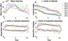 |
Fig. 3. Properties of observed active regions with a lifetime of less than seven days calculated for northern and southern wings of cycles 21–24. Values are yearly means and the first year of each wing starts from the emergence of the first active region of that wing. Top left panel: mean total unsigned flux. Top right panel: limits of plus and minus one standard deviation around mean latitude. Bottom left panel: limits of plus and minus one standard deviation around mean latitude separation of polarities. Bottom right panel: limits of plus and minus one standard deviation around mean longitude separation of polarities. Different colors mark different cycles. Solid lines are for northern wings; dashed lines for southern wings. |
We then create additional active regions for the far-side of the Sun using these statistical properties. Since the distributions of latitude and the polarity separations in latitude and longitude are roughly Gaussian, we determined the latitude and the polarity separations of the additional active regions by drawing random numbers from Gaussian distributions with the same means and standard deviations as the observed active regions. The flux distribution is close to exponential, so the fluxes of the additional active regions were drawn from an exponential distribution with the mean calculated from the observed active regions.
While this method provides a rough estimate of flux emergence on the far-side of the Sun, a few notable shortcomings should be noted. The mean latitude, the latitude and longitude separations, and the flux were treated as independent variables, even though they are not strictly independent. Also, because the properties of the additional active regions were selected randomly from probability distributions, some of them have a lifetime that is longer than the lifetime limit. The method allows the formation of anti-Hale active regions, but under the assumption that their properties follow the same distributions as the properties of active regions that obey Hale’s polarity law.
Once the total flux and the locations of positive and negative polarity parts of an additional active region were determined, the active region was constructed using the method that is shortly discussed below and was used in Virtanen et al. (2017), where it was shown that using additional active regions constructed with the method in an SFT simulation instead of observed active regions does not change the simulated magnetic field significantly.
Circles of negative and positive polarity were placed at the locations of the negative and positive polarity parts of the active region, respectively. The area of the circles was determined by calculating the number of pixels with an intensity of 200G that would be required to reach the total flux of the active region. A two-dimensional Gaussian distribution was then placed in each circle, noise was added to the distributions and they were then normalized so that there are equal amounts of negative and positive flux, and the total unsigned flux inside them matches the total unsigned flux determined for the additional active region. For a more detailed explanation and an example, see Virtanen et al. (2017).
6. Simulated magnetic field
The top panel of Fig. 4 shows a supersynoptic map from a simulation where additional active regions were inserted to the far-side of the Sun in addition to the observed active regions in the front side. The lifetime limit of the additional active regions was four days. For comparison, the bottom panel of Fig. 4 shows a supersynoptic map from a simulation that contained only the observed active regions. All simulations in this paper were initiated with a synoptic map that has a magnetic field of ±2.5G in the polar areas above 60° and below −60° latitude and is zero elsewhere. This serves as an approximation of the polar fields in early 1975. An observed synoptic map was not used due to errors in polar fields in the early NSO/KP data.
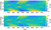 |
Fig. 4. Supersynoptic maps from two SFT simulations. In the top panel, additional active regions are inserted to the far-side of the Sun using a lifetime limit of four days. In the bottom panel, only observed active regions are used as input. |
The most visible difference between the two simulations is the polar field strength. The additional far-side flux is partly transported to the poles, creating stronger magnetic fields, especially near solar minima. At lower latitudes, the differences are more subtle. The additional active regions have not created any notable additional poleward surges of flux. The strength of the existing surges has in some cases slightly changed, but their locations and timings remain practically identical. The surges are mainly created by large active regions, which typically have long lifetimes and are always observed on the near-side of the Sun at some point of their evolution. The additional active regions with short lifetimes are not capable of creating visible flux surges. Instead they seem to create a weak continuous flow of flux that strengthens the polar field, but this effect is not easily detected at low latitudes or in short timescales, where large active regions dominate the evolution of the magnetic field.
Figure 5 shows the average strength of the polar fields above 60° and below −60° latitude from six different simulations. The dashed lines depict a simulation that contains only the observed active regions. The solid black lines show the five simulations that include additional activity on the far-side constructed with a lifetime limit of four days. The five different pairs of black lines correspond to the polar fields of five different simulation runs, where the yearly statistical distributions of the properties of the additional active regions were the same, but the properties of individual active regions were taken randomly from the distributions for each run. Hence the black curves give us an estimate of how much the missed active regions on the far-side of the Sun could affect the evolution of the polar fields. The red and blue crosses depict the observed northern and southern polar fields determined from the synoptic maps.
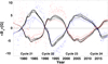 |
Fig. 5. Average strength of polar fields above 60° and below −60° latitude from six SFT simulations. The dashed lines depict a simulation that included only observed active regions. The solid black lines show five simulations that included additional far-side active regions with a lifetime limit of four days. The red and blue crosses are observed values of the northern and southern polar fields determined from synoptic maps. |
Figure 5 shows that the significance of the additional far-side flux depends on the cycle, the cycle phase and the properties of the simulation run. This is most clearly seen close to solar minimum times, when the polar fields are strongest. The maximum absolute polar field strength tends to be 1G − 3G higher when far-side flux is added. The southern hemisphere of cycle 21 shows the largest increase in maximum field strength, from about 4G to about 7G. The difference between different simulation runs with far-side activity is in all wings at most about 1G. Maximum times are affected to a much lesser degree. The polarity reversals of cycles 22 and 23 tend to happen up to a few months later when far-side flux is added. In cycle 24, the polarity reversal can happen either earlier or later compared to the reference simulation, depending on the simulation run. The polarity reversal of cycle 21 happens a few months earlier when far-side flux is added. This is likely to be because all simulations start from the same polar fields. The additional flux in the ascending phase of cycle 21 causes a faster polarity reversal in that cycle. However, in later cycles this effect does not affect the stronger polar fields.
Figure 6 shows polar fields from the reference simulation and five simulations with additional far-side flux similar to Fig. 5, but the lifetime limit of the far-side active regions is seven days instead of four, implying that more far-side flux is added. The minimum time field strength is now significantly higher than in Fig. 5, reaching 8G − 9G in several wings. The effects in maximum times are also similar but somewhat stronger than seen in Fig. 5. The polarity reversals of especially cycles 23 and 24 are now more clearly delayed. The maximum delay is about a year.
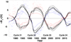 |
Fig. 6. Average strength of polar fields above 60° and below −60° latitude from six SFT simulations. The dashed lines depict a simulation that included only observed active regions. The solid black lines show five simulations that included additional far-side active regions with a lifetime limit of seven days. The red and blue crosses are observed values of the northern and southern polar fields determined from synoptic maps. |
To assess the accuracy of the simulations we calculated the mean squared error between the observed polar field strength and the simulations. The mean is taken over both hemispheres, and in the case of the simulations with additional active regions also over all simulation runs. In the simulation, when using only observed active regions, the mean squared error was 11.4G2, in the simulation using additional active regions with a lifetime limit of four days 9.3G2, and in the simulation using additional active regions with a lifetime limit of seven days 8.6G2. This means that as more additional active regions were added to the far-side, the average difference between simulations and observations became smaller, implying, furthermore, that the accuracy of the simulations was increased.
Table 1 shows the error values separately for northern and southern hemispheres and for cycles 21–24. The starting times of cycles 22–24 were taken to be September 1986, August 1996 and December 2008, respectively. Cycles 21 and 24 are incomplete, because the data set does not cover the beginning of cycle 21 or the ending of cycle 24. There is significant variation between cycles. Cycle 21 shows larger errors when far-side flux is added, but it is also heavily affected by erroneous data, as seen in Figs. 5 and 6. In the simulations, cycle 21 also suffers from initialisation effects, as discussed above. In cycles 22 and 23, the match between observations and simulations is significantly improved when additional active regions are added. In cycle 24, an improvement is also seen when a lifetime limit of four days is used. Raising the limit to seven days does not lead to further improvement in the southern hemisphere and, in fact, this makes the mean squared error considerably larger in the northern hemisphere. This is caused by larger deviations from observations in the ascending phase of the cycle. We note that while the simulations never quite reached the observed polar field strengths in the two earlier minima, they tend to lead to larger strengths during the minimum between cycles 23 and 24. After the polarity reversal, the simulations with a lifetime limit of seven days leads to much better agreement with observations than with the simulation without additional active regions, as can be seen in Fig. 6.
Mean squared error of northern and southern polar field strength in cycles 21–24 in a simulation without additional active regions, a simulation including additional active regions with a lifetime limit of four days, and a simulation including additional active regions with a lifetime limit of seven days.
These findings agree well with the results of Virtanen et al. (2017), where we found that in simulations based only on the observed active regions, the simulated polar field strength is lower than the observed polar field strength in minimum times, and the polarity reversals of cycles 22 and 23 are earlier in the simulations than the observations. The far-side flux brings the simulation closer to observations. Because of the uncertainties in minimum time field strength caused by the far-side active regions, the missing flux could also explain differences in the relative strength of minimum time polar fields of different cycles between the simulations and observations.
7. Conclusions
Here, we study the lifetimes of active regions using both SFT simulations and full-disk magnetographic observations. We found a similar dependence between lifetime and the amount of total unsigned flux required for it in simulations and observations. We also determined the statistical distributions of active region properties for each year of each solar cycle wing and used them to create additional active regions that are similar to the observed active regions in all cycles and cycle phases.
We inserted the additional active regions to the far-side of the Sun in SFT simulations. We used the number of observed near-side active regions and their lifetimes to determine the number of additional active regions on the far-side, adding regions whose lifetimes are short enough so that they could be missed by an observer looking only at the near-side. We found that the additional flux can produce significantly stronger polar fields in minimum times and slightly later polar field reversals near maxima. The size of the effect depends on the cycle, the hemisphere, and the properties of the individual active regions, which are randomly selected from the related probability distributions.
The mechanism by which the additional far-side active regions affect the evolution of the polar fields is a weak flow of flux, which is not clearly visible at low latitudes or in short time scales, but accumulates flux at the poles over the years. The flow is not strong enough to create new poleward surges of flux at mid-latitudes, but it can visibly strengthen already existing surges.
We found that the additional flux tends to result in simulations that agree better with observations. We have previously noted (Virtanen et al. 2017) that in minimum times, SFT simulations tend to create weaker polar fields than observed and that the polarity reversals of cycles 22 and 23 are slightly earlier than observed. The results of this paper show that adding far-side flux can increase the maximum polar field strength and move the polarity reversal timings to the correct direction without changing the main characteristics of the solar cycle, such as the poleward flux surges, or causing other new errors.
However, the exact number and the properties of the far-side active regions are not known very well, and cannot be accurately determined from the synoptic maps used in this study. In addition to the completely hidden far-side active regions, some near-side active regions are also invisible in synoptic maps. A more detailed analysis of full-disk magetograms will be required to give an accurate estimate of the number of missed active regions.
Accordingly, far-side solar activity is essential for understanding the long-term evolution of solar magnetic fields. Recently, several authors (e.g., Virtanen et al. 2019) demonstrated that each cycle, the dipole moment of the Sun is determined by a relatively small number of active regions. What we find here is that the contribution of small short-lived active regions cannot be neglected. Adding flux from these regions, which emerge and decay on the far-side of the Sun markedly improves the agreement with the observed polar flux. While estimates of far-side activity based on front-side observations, as done in this study, can partly remedy the situation, observations from the far-side of the Sun would be an important addition for a better understanding of space climate and for an improved forecasting of space weather.
References
- Baumann, I., Schmitt, D., Schüssler, M., & Solanki, S. K. 2004, A&A, 426, 1075 [NASA ADS] [CrossRef] [EDP Sciences] [Google Scholar]
- Baumann, I., Schmitt, D., & Schüssler, M. 2006, A&A, 446, 307 [NASA ADS] [CrossRef] [EDP Sciences] [Google Scholar]
- Beck, J. G., Gizon, L., & Duvall, T. L. Jr. 2002, ApJ, 575, L47 [NASA ADS] [CrossRef] [Google Scholar]
- Howard, R. 1974, Sol. Phys., 38, 283 [NASA ADS] [CrossRef] [Google Scholar]
- Jiang, J., Cameron, R., Schmitt, D., & Schüssler, M. 2010, ApJ, 709, 301 [NASA ADS] [CrossRef] [Google Scholar]
- Jiang, J., Cameron, R. H., Schmitt, D., & Schüssler, M. 2011, A&A, 528, A82 [NASA ADS] [CrossRef] [EDP Sciences] [Google Scholar]
- Jones, H. P., Duvall, T. L. Jr., Harvey, J. W., et al. 1992, Sol. Phys., 139, 211 [NASA ADS] [CrossRef] [Google Scholar]
- Keller, C. U., Harvey, J. W., & Giampapa, M. S. 2003, in Innovative Telescopes and Instrumentation for Solar Astrophysics, ed. S. L. Keil, & S. V. Avakyan, Proc. SPIE, 4853, 194 [NASA ADS] [CrossRef] [Google Scholar]
- Livingston, W. C., Harvey, J., Slaughter, C., & Trumbo, D. 1976, Appl. Opt., 15, 40 [NASA ADS] [CrossRef] [Google Scholar]
- Pevtsov, A. A., Bertello, L., Nagovitsyn, Y. A., Tlatov, A. G., & Pipin, V. V. 2021, J. Space Weather Space Clim., 11, 4 [CrossRef] [EDP Sciences] [Google Scholar]
- Pietarila, A., Bertello, L., Harvey, J. W., & Pevtsov, A. A. 2013, Sol. Phys., 282, 91 [NASA ADS] [CrossRef] [Google Scholar]
- Riley, P., Ben-Nun, M., Linker, J. A., et al. 2014, Sol. Phys., 289, 769 [Google Scholar]
- Scherrer, P. H., Wilcox, J. M., Svalgaard, L., et al. 1977, Sol. Phys., 54, 353 [NASA ADS] [CrossRef] [Google Scholar]
- Ulrich, R. K. 2010, ApJ, 725, 658 [NASA ADS] [CrossRef] [Google Scholar]
- Ulrich, R. K., & Boyden, J. E. 2005, ApJ, 620, L123 [NASA ADS] [CrossRef] [Google Scholar]
- Ulrich, R. K., & Tran, T. 2013, ApJ, 768, 189 [NASA ADS] [CrossRef] [Google Scholar]
- Virtanen, I., & Mursula, K. 2017, A&A, 604, A7 [NASA ADS] [CrossRef] [EDP Sciences] [Google Scholar]
- Virtanen, I. O. I., Virtanen, I. I., Pevtsov, A. A., Yeates, A., & Mursula, K. 2017, A&A, 604, A8 [NASA ADS] [CrossRef] [EDP Sciences] [Google Scholar]
- Virtanen, I. O. I., Virtanen, I. I., Pevtsov, A. A., & Mursula, K. 2018, A&A, 616, A134 [NASA ADS] [CrossRef] [EDP Sciences] [Google Scholar]
- Virtanen, I. O. I., Virtanen, I. I., Pevtsov, A. A., & Mursula, K. 2019, A&A, 632, A39 [CrossRef] [EDP Sciences] [Google Scholar]
- Whitbread, T., Yeates, A. R., Muñoz-Jaramillo, A., & Petrie, G. J. D. 2017, A&A, 607, A76 [NASA ADS] [CrossRef] [EDP Sciences] [Google Scholar]
- Yeates, A. R., Baker, D., & van Driel-Gesztelyi, L. 2015, Sol. Phys., 290, 3189 [NASA ADS] [CrossRef] [Google Scholar]
All Tables
Mean squared error of northern and southern polar field strength in cycles 21–24 in a simulation without additional active regions, a simulation including additional active regions with a lifetime limit of four days, and a simulation including additional active regions with a lifetime limit of seven days.
All Figures
|
Fig. 1. Latitude and observation time of identified active regions. Different solar cycle wings have been marked with different colors for clarity. |
| In the text | |
|
Fig. 2. Relationship between active region lifetime and total magnetic flux. Middle panel: simulated and observed lifetimes of active regions as functions of their total unsigned flux. Blue markers are simulated lifetimes obtained from SFT simulations using NSO/SOLIS and HMI synoptic maps. Red markers are observed lifetimes obtained from SOLIS full-disk magnetograms. The solid blue and red curves show the median flux in lifetime bins with a width of one day for simulated and observed lifetimes, respectively. The blue and red bars on the left and right show the number of active regions in each bin. |
| In the text | |
|
Fig. 3. Properties of observed active regions with a lifetime of less than seven days calculated for northern and southern wings of cycles 21–24. Values are yearly means and the first year of each wing starts from the emergence of the first active region of that wing. Top left panel: mean total unsigned flux. Top right panel: limits of plus and minus one standard deviation around mean latitude. Bottom left panel: limits of plus and minus one standard deviation around mean latitude separation of polarities. Bottom right panel: limits of plus and minus one standard deviation around mean longitude separation of polarities. Different colors mark different cycles. Solid lines are for northern wings; dashed lines for southern wings. |
| In the text | |
|
Fig. 4. Supersynoptic maps from two SFT simulations. In the top panel, additional active regions are inserted to the far-side of the Sun using a lifetime limit of four days. In the bottom panel, only observed active regions are used as input. |
| In the text | |
|
Fig. 5. Average strength of polar fields above 60° and below −60° latitude from six SFT simulations. The dashed lines depict a simulation that included only observed active regions. The solid black lines show five simulations that included additional far-side active regions with a lifetime limit of four days. The red and blue crosses are observed values of the northern and southern polar fields determined from synoptic maps. |
| In the text | |
|
Fig. 6. Average strength of polar fields above 60° and below −60° latitude from six SFT simulations. The dashed lines depict a simulation that included only observed active regions. The solid black lines show five simulations that included additional far-side active regions with a lifetime limit of seven days. The red and blue crosses are observed values of the northern and southern polar fields determined from synoptic maps. |
| In the text | |
Current usage metrics show cumulative count of Article Views (full-text article views including HTML views, PDF and ePub downloads, according to the available data) and Abstracts Views on Vision4Press platform.
Data correspond to usage on the plateform after 2015. The current usage metrics is available 48-96 hours after online publication and is updated daily on week days.
Initial download of the metrics may take a while.