| Issue |
A&A
Volume 652, August 2021
|
|
|---|---|---|
| Article Number | A50 | |
| Number of page(s) | 14 | |
| Section | Astronomical instrumentation | |
| DOI | https://doi.org/10.1051/0004-6361/202140376 | |
| Published online | 10 August 2021 | |
Blind restoration of solar images via the Channel Sharing Spatio-temporal Network
1
Institute of Optics and Electronics Chinese Academy of Sciences, Chengdu, PR China
e-mail: This email address is being protected from spambots. You need JavaScript enabled to view it.
2
University of Electronic Science and Technology of China, Chengdu, PR China
e-mail: This email address is being protected from spambots. You need JavaScript enabled to view it.
3
Key Laboratory on Adaptive Optics, Chinese Academy of Sciences, Chengdu, PR China
4
University of Chinese Academy of Sciences, Beijing, PR China
5
Yangtze Delta Region Institute of University of Electronic Science and Technology of China, Quzhou, PR China
Received:
19
January
2021
Accepted:
31
May
2021
Abstract
Context. Due to the presence of atmospheric turbulence, the quality of solar images tends to be significantly degraded when observed by ground-based telescopes. The adaptive optics (AO) system can achieve partial correction but stops short of reaching the diffraction limit. In order to further improve the imaging quality, post-processing for AO closed-loop images is still necessary. Methods based on deep learning (DL) have been proposed for AO image reconstruction, but the most of them are based on the assumption that the point spread function is spatially invariant.
Aims. Our goal is to construct clear solar images by using a sophisticated spatially variant end-to-end blind restoration network.
Methods. The proposed channel sharing spatio-temporal network (CSSTN) consists of three sub-networks: a feature extraction network, channel sharing spatio-temporal filter adaptive network (CSSTFAN), and a reconstruction network (RN). First, CSSTFAN generates two filters adaptively according to features generated from three inputs. Then these filters are delivered to the proposed channel sharing filter adaptive convolutional layer in CSSTFAN to convolve with the previous or current step features. Finally, the convolved features are concatenated as input of RN to restore a clear image. Ultimately, CSSTN and the other three supervised DL methods are trained on the binding real 705 nm photospheric and 656 nm chromospheric AO correction images as well as the corresponding speckle reconstructed images.
Results. The results of CSSTN, the three DL methods, and one classic blind deconvolution method evaluated on four test sets are shown. The imaging condition of the first photospheric and second chromospheric set is the same as training set, except for the different time given in the same hour. The imaging condition of the third chromospheric and fourth photospheric set is the same as the first and second, except for the Sun region and time. Our method restores clearer images and performs best in both the peak signal-to-noise ratio and contrast among these methods.
Key words: Sun: photosphere / methods: data analysis / techniques: image processing
© ESO 2021
1. Introduction
The presence of atmospheric turbulence causes serious wavefront distortions of the light waves and affects observations of certain objects by ground-based telescopes. As a result, the imaging resolution of the ground-based telescope on the object is far below the expected theoretical diffraction limit, seriously affecting the imaging quality. These effects are particularly severe situation when observing the Sun from Earth.
As a way of mitigating these problems, ground-based telescopes normally use Adaptive Optics (AO) technology (Babcock 1953; Rimmele 2000; Scharmer et al. 2000; Wenhan et al. 2011) to compensate for the influence of atmospheric turbulence. The AO system consists of wavefront detector, wavefront corrector, and wavefront controller. The AO process generally measures atmospheric disturbances through a wavefront sensor and compensates the wavefront distortion caused by atmospheric turbulence through a deformable mirror in real time. The AO technology can significantly reduce low-order aberrations, effectively improving the imaging quality of the optical system. Therefore, AO is widely used in high-resolution imaging of ground-based telescopes (Rousset et al. 1990; Rao et al. 2003, 2015, 2016, 2020; Ellerbroek et al. 2005; Johns et al. 2012) as well as laser systems (Jiang et al. 1989) and ophthalmology fields (Liang et al. 1997; Roorda & Williams 1999).
However, due to the hardware limitations of the AO system, the correction of wavefront distortion is partial and incomplete, and, thus, the high-frequency data for the object is largely lost. In order to further improve the imaging quality of the AO image, the post-processing of AO image is generally essential. Currently, there are three main post-processing methods applied to AO images.
The first type is based on speckle imaging technology (De Boer et al. 1992; Von der Lühe 1993), which reconstructs the phase and amplitude of the object using the statistical characteristics of atmospheric turbulence. A great deal of research (Keller & Von Der Luehe 1992; Von der Luehe 1994; Janßen et al. 2003; Sütterlin et al. 2004; Al et al. 2004; Denker et al. 2005; Zhong et al. 2014) has demonstrated that speckle imaging technology has achieved good results in the study of small solar structures. However, in order to take full advantage of the statistical information of atmospheric turbulence, this method usually requires hundreds of short-exposure degraded images to complete an image reconstruction (Denker et al. 2001).
The second type is the phase diversity (PD) method (Gonsalves 1982; Paxman et al. 1992; Löfdahl & Scharmer 1994; Berger et al. 1998; Tritschler & Schmidt 2002; Scharmer et al. 2002; Löfdahl et al. 2004; Zhang et al. 2017), which employs a set made up of a focused image and a defocused image to build the error metric. The PD method is not only capable of reconstructing a clear image of the degraded object, but it can also obtain the point spread function (PSF) of the object degradation by minimizing the error metric. The most successful and effective method is the multiple objects multi-frame blind deconvolution (MOMFBD; Van Noort et al. 2005), which can jointly restore multiple realizations of multiple objects with known wavefront relationships. However, the limitation of MOMFBD lies in the extensive calculations involved. Because this technology requires an additional imaging device and the algorithm is sensitive to system parameters, there are still some technical difficulties with regard to its practical application.
The third one is the image blind deconvolution (BD) algorithm (Lane 1992; Schulz 1993; Tsumuraya et al. 1994), which reconstructs the object and PSF from noisy blurry images simultaneously. Since it is a severely ill-posed inverse problem, the BD algorithm normally requires prior information to constrain the solution. A large number of blind deconvolution algorithms have been proposed in recent years. Chan & Wong (1998), Sidky & Pan (2008) proposed BD algorithms based on total variation blind deconvolution. Perrone & Favaro (2014) reveal the key details of TV-based blind deconvolution methods (TVBD) and introduce an adaptation of Chan & Wong (1998). Holmes (1992), Thiébaut & Conan (1995), Levin et al. (2011) proposed BD algorithms based on maximum likelihood estimation. Krishnan et al. (2011) present a normalized sparsity prior that favors clear images over blurred ones. Molina et al. (2006) proposed a model parameter estimation BD algorithm. Because BD has no special requirements for the imaging system, it is the most effective and widely applicable image post-processing technology and also the most flexible in its practical application (Ayers & Dainty 1988; Campisi & Egiazarian 2017).
Because observations are generally continuous within the generated time of many short exposure AO images, multiframe blind deconvolution algorithms have received more and more attention, which recovers fixed latent objects and corresponding PSFs from multiple observations simultaneously. Löfdahl (2002) proposed multiframe blind deconvolution with linear equality constraints and Yu et al. (2009) proposed multiframe blind deconvolution based on frame selection.
With the rapid development of deep learning in recent years, this technology has also been used with growing frequency in astrophysics, as well as biomedicine with AO, apart from a large number of applications in computer vision and natural language processing. Gravet et al. (2015) achieved their classification of the morphology of the Milky Way using deep learning in astrophysics. Xiao et al. (2017) restore human eye retina images via a simple convolutional neural network (Retinal-CNN) in the field of biomedicine with AO. In the field of solar AO, Asensio Ramos et al. (2017) infers the horizontal velocity field of the sun surface, Diaz Baso & Asensio Ramos (2018) simultaneously deconvolve and super-resolve images and magnetograms, while Asensio Ramos et al. (2018) deconvolve solar AO image. Asensio Ramos et al. (2018) proposed two different architectures. One is the encoder-decoder deep neural network (ED-DNN), which constructs a clear frame from every seven burst frames, with the limitation, however, that ED-DNN can only process burst images with a fixed number of frames. The other is the recurrent deep neural network (Recurrent-DNN), which can construct an intermediate deconvolved image from two frames out of every burst of images. Recurrent-DNN can work with an arbitrary number of frames and has information transmission within burst images. For ED-DNN and Recurrent-DNN, every batch of burst of images is processed separately, so there is no information transmission from batch to batch. In addition, these methods only use the mean square error (MSE) loss, which tends to produce unnatural images when the number of frames is small since MSE is only concerned with the quantity of pixels.
Diaz Baso et al. (2019) correct noisy narrowband polarisation data using deep learning. Asensio Ramos & Olspert (2021) estimate the object and PSF from multiple noisy blurry images using unsupervised deep learning simultaneously. Armstrong & Fletcher (2021) correct atmospheric seeing in solar flare observations using deep learning. Asensio Ramos & Olspert (2021) correct point-like objects as well as extended objects using unsupervised deep learning.
The methods based on deep learning are all realized by learning the end-to-end network. Once the supervised or unsupervised network is trained, clear images can be swiftly reconstructed by these network.
Although methods based on deep learning have achieved good results in the AO field, most of the above-cited methods (Xiao et al. 2017; Asensio Ramos et al. 2018) all assume that the PSF of input image is spatially invariant. In actual AO imaging process, the assumption of that the PSF is spatially invariant is usually invalid due to the existence of the anisoplanatism effect in the optic path. These effects hamper the spatially invariant method to recover a whole latent image simultaneously. In order to get the whole restoration image, these methods must follow the standard approach of dividing the image into different isoplanatic patches and applying this tool to each one of them. The biggest limitation of these methods is that a different network parameter needs to be trained for each isoplanatic patch. In order to reconstruct different isoplanatic blocks in a single network, these methods need to learn more complex mapping between a blurred image and the clear image, leading to more difficult or time-consuming training and a weaker robustness of the network.
In contrast to the spatially invariant network methods above, Zhou et al. (2019) proposed an Spatio-Temporal Filter Adaptive Network (STFAN) for video deblurring. The STFAN contains a Filter Adaptive Convolutional (FAC) layer, which utilizes the deblurred information from the previous image to the current image in video. Thus, STFAN conducts an information transmission over time. In addition, STFAN generated both the spatially variant alignment filters and deblurring filters; thus, this network is able to learn to simultaneously generate the corresponding PSFs for every individual isoplanatic block. As a result, STFAN is more adept at learning to map every isoplanatic block of the whole image in one network simutanously, making the network learning process more simple and robust.
In this paper, we achieve a blind restoration of solar images using an end-to-end channel sharing spatio-temporal network (CSSTN) based on STFAN (Zhou et al. 2019). Here, CSSTN undergoes three main improvements in comparison with STFAN, while it transfers the natural scene video deblurring to AO multiframe image deblurring. These include: (1) sharing filters throughout each channel, inspired by the fact that a receptive field of adaptive filters can cover the AO isotropic patch; (2) using a smaller but fully spatially variant filter size according to an AO image process; and (3) adding symmetric skip connections between the sub-networks so that the vanishing gradient can be largely overcome. The proposed network can deblur the spatially variant images efficiently. Once the network is trained, only two consecutive time short exposure frames are used to quickly reconstruct high-quality clear images with arbitrary size in the inference process. Our method restores sharper images and performs best at both a peak signal-to-noise ratio (PSNR) and contrast compared with several existing optical image blind deconvolution methods that are based on deep learning.
The paper is organized as follows. In Sect. 2, we show the structure of the proposed networks and training implementation details. Section 3 presents the images, evaluation, and discussion of results. Section 4 presents the main conclusions and prospects for a future work.
2. Channel sharing spatio-temporal network
2.1. Network structure
As shown in Fig. 1, a channel sharing spatio-temporal network (CSSTN) consists of three sub-networks: a feature extraction network, a channel sharing spatio-temporal filter adaptive network (CSSTFAN), and a reconstruction network. It is worth noting that we use multiple residual blocks in the network, which makes network optimization easier and stable. We not only add a shortcut connection between the input and output, but also add a symmetric skip connection (Mao et al. 2016) between the feature extraction network and the reconstruction network. The vanishing gradient can be largely overcome by these symmetric skip connections, which helps to build and optimize the network better, making deep network learning easier, and thus achieving the improvement of recovery performance.
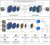 |
Fig. 1. Proposed deep neural network architecture. Panel a: shows our proposed channel sharing spatio-temporal network (CSSTN). Panel b: is a channel sharing spatio-temporal filter adaptive network (CSSTFAN) sub-network. Panel c: is the meaning of different color blocks and symbols in the network. CSSTN consists of three sub-networks: a feature extraction network, a CSSTFAN, and a reconstruction network. Firstly the feature extraction network extracts features Et from the current blurry image Bt. Given the blurred image Bt − 1 and restored image Rt − 1 of the previous time step, and current input image Bt, the CSSTFAN generates the Fsvi and Fsvc in order. Using CSFAC layer ⊛, CSSTFAN convolves Fsvi with features Ht − 1 of the previous time step and convolves Fsvc with features Et. Finally, the reconstruction network restores the latent image from the fused features Ct. k denotes the filter size of CSFAC layer and it is 3 in our final network. |
The feature extraction network contains three superblocks, and each superblock consists of a convolutional layer and three residual blocks, as shown in Fig. 1a. Both the convolutional layer and the residual block (He et al. 2016) act as feature extractors, capturing high-level features of the image content. The activation function of each residual block is LeakyReLU (Maas et al. 2013). The properties of these super blocks (numbered as Ci, j in Fig. 1a) are shown in Table 1, while i refers to the superblock and j to the block inside the superblock (Asensio Ramos et al. 2018). The feature extraction network extracts features Et (t is image index) from the current blurry image Bt. The Et are used as the input for CSSTFAN.
Architecture of feature extraction sub-network and reconstruction sub-network.
It is worth noting that the kernel size of each convolutional layer is 5 × 5, instead of 3 × 3, because in our experience this helps to include a larger number of proper image details in the process of reducing the feature size and to make the restored image clearer.
As shown in Fig. 1b, CSSTFAN takes the previous blurred image Bt − 1, the previous restored image Rt − 1 and the current blurred image frame Bt as input. It’s worth noting that Bt − 1 and Rt − 1 are initialized to B1 in the case t = 1 for each sequence. The encoder gencoder extracts feature Tt from the triple inputs. The gencoder consists of three super blocks, and each of them consists of a convolutional layer and three residual blocks. The activation function of each residual block is LeakyReLU. The properties of these super blocks are shown in Table 2. The generator gsvi (sv for spatial variant, i for inter-frame) takes the features Tt extracted by the gencoder as input, and generates the spatially variant filter  (h is height of feature map, w is width of feature map, k is the blur kernel size of the learned spatially variant filter) for the inter-frame adjustment between the previous frame and the current frame. Here, Fsvi contains a large amount of inter-frame information, which may help the neural network successfully compensates the miss alignment between the images. The Fsvi and Tt are concatenated as the input of the generator gsvc (c for current frame) and, finally, the filter
  is generated. This process can be expressed as:
 (1)
(1)
 (2)
(2)
Architecture of channel sharing spatio-temporal filter adaptive network (CSSTFAN) sub-network.
Both gsvi and gsvc generator consist of two convolutional layers and two residual blocks. The number of channels in the first convolutional layer is 128, and the number of channels in the second convolutional layer is k2. The Fsvi is applied to the previous deblurring feature Ht − 1 and can adjust the deblurring feature of the previous time step with the current frame. The Fsvc is applied to the features Et of the current blurred frame extracted by the feature extraction network. Finally, the both filtered results are concatenated to obtain the feature Ct. Ct is the input of the reconstruction network. After Ct going through a convolutional layer, the deblurring feature Ht is transferred to the follow-up CSSTFAN. The process can be expressed as:
 (3)
(3)
 (4)
(4)
 (5)
(5)
 (6)
(6)
where Concate( ⋅ , ⋅ ) is channel concatenation operator, Fea( ⋅ ) is convolution operator, whose kernel size is 3 × 3 and stride is 1.
CSSTFAN takes the previous blurred image Bt − 1, the previous restored image Rt − 1, and the current frame Bt as input for learning inter-frame filters and current-frame filters. Implicit relations between Bt − 1 and Bt contains a lot of inter-frame information, which is helpful for learning spatially variant inter-frame filters. Connection between Bt − 1 and Rt − 1 implies a lot of deblurring information, which is helpful for learning spatially variant current-frame filters.
The reconstruction network takes the concatenated features Ct as input to restore a latent image Rt. The reconstruction network contains three super blocks, and both the first and the second super blocks contain three residual blocks and a deconvolution layer. The last super block contains three residual blocks and a convolutional layer. The properties of these super blocks are shown in Table 1.
Inspired by the STFAN (Zhou et al. 2019) method applied in the field of video deblurring, we now propose a channel sharing spatio-temporal filter adaptive network (CSSTFAN) sub-network. Unlike the dynamic filter network (Jia et al. 2016; Mildenhall et al. 2018), which applies the generated spatially variant filters directly to the input image, STFAN generates spatially variant filters for each channel and our proposed channel sharing filter adaptive convolutional (CSFAC) layer applies the generated spatially variant filters on down-sampled features and shares filters among each channel. It makes a smaller filter and a reasonable larger receptive field.
Unlike the standard multiframe image blind deconvolution method (Asensio Ramos et al. 2018) in which ED-DNN takes seven consecutive blurred frames as input to restore the clear frame, our network only uses the previous blurred frame, the previous restored frame, and the current blurred frame as input. A large amount of information from the previous frame is used without increasing the extent of the calculations.
In CSSTN, the generated filter is only different in each position, and same in each channel. In theory, the channel sharing filter is four-dimensional (h × w × k × k). In practice, the generated filter is h × w × k2. First, we reshape it to four-dimensional (h × w × k × k) and then we apply the filter to each channel of the feature. The CSFAC layer structure is shown in Fig. 2. For the input feature Q ∈ ℝh × w × c (c is channel number of feature map) and the generated filter, F ∈ ℝh × w × k2, each specific filter,  , (reshape from 1 × 1 × k2) is applied to each channel of the input feature position (x, y), which can be expressed as:
 (7)
(7)
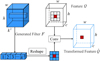 |
Fig. 2. Proposed channel sharing filter adaptive convolutional layer (CSFAC). The generated filter F is h × w × k2. We reshape it to h × w × k × k, and then apply the filter to each channel of the feature Q, finally get transformed feature |

where ci is the ith channel of the feature Q,  , * is the convolution operator, Qx, y, ci and
  is the input feature and transformed feature of the position (x, y, ci), respectively.
The standard kernel prediction network methods (Jia et al. 2016; Mildenhall et al. 2018) have to predict larger filters for each pixel of the input image, which requires large computational cost and memory. In contrast, the proposed network does not require a large filter size due to the use of CSFAC layer on down-sampled features (Zhou et al. 2019).
2.2. Loss function
In order to make the restored image and the training clear image consistent in not only low-level pixel values, but also high-level abstract features and overall conceptual style, we used two kinds of loss function. One is pixel-based mean square error loss (MSE), and the other is the feature-based perceptual loss (Johnson et al. 2016).
MSE is used to measure the difference between the restored image R and the training clear image G:
where C, H, W are the image dimensions.
The perceptual loss is defined as the Euclidean distance of output from the pretrained Vgg-19 network feature map (Johnson et al. 2016) of R and G:
where Φj denotes the features from the jth convolutional layer of the pretrained VGG-19 network, Cj, Hj, Wj are the dimensions of the jth feature map. In this paper, we use the weighted average of the 3rd, 8th, and 15th feature maps (conv1-2, conv2-2, conv3-3) output, while the weights are 1, 0.2, 0.04, respectively, according to Zhou et al. (2019). The perceptual loss can be formulated as:

The final loss function for the proposed network is defined as:
where λ is the balance factor of MSE loss and perception loss, and it is set as 0.01 in our experiment (Zhou et al. 2019).
2.3. Training
We trained the proposed deep neural network1 with binding photospheric 705 nm data and chromospheric 656 nm data. The AO closed-loop images dataset observed with New Vacuum Solar Telescope (NVST; Kong et al. 2016, 2017), which is a one-meter vacuum solar telescope located by Fuxian Lake in southwest China. The data was observed with ground layer adaptive optics (GLAO) prototype system (Kong et al. 2016, 2017) and classical adaptive optics (CAO) prototype system. These TiO (705 nm) band images of active region NOAA 12599 were observed by the GLAO system around the time [UT] 5:35:55, October 7, 2016, with an angular pixel size of 34.5 milliarcsec. These 656 nm band images of active region NOAA 12598 observed by the CAO system around the time [UT] 3:36, October 7, 2016, with an angular pixel size of 130 milliarcsec.
We use the results of solar speckle reconstruction image (Zhong et al. 2014) as supervision. The speckle reconstruction method uses 100 frames of blurred images to restore one clear image. In our experiment, there are a total of 6700 photospheric AO closed-loop short exposure images with 1.5 ms exposure time and 67 corresponding speckle reconstruction images pair. The image size is 1792 × 1792. We divide the data into a 5700 pairs training set and a 1000 pairs testing set. In addition, there are a total of 100 chromospheric AO closed-loop short exposure images with a 10 ms exposure time and one corresponding speckle reconstruction image pair. The size of these images is 512 × 512. We divide the data into a training sets of 80 pairs and a test sets of 20 pairs. In order to maintain the balance of the two training samples, we copy the chromosphere data 80 times to finally obtain 6400 pairs training set.
The training dataset was augmented in order to train the network to have better generalization capabilities. To facilitate training, we divide all burst frames into sequences of a length of 20. The training data set are randomly cropped into 256 × 256 pixel block. The augmenting strategy consists of randomly flipping the images horizontally and vertically. In order to prevent overfitting, the training data set is randomly shuffled before each training. All of the above data augmentation methods increase the generalization capabilities of neural networks.
We train the proposed network on a computer with an Intel i7-8700K CPU with 16 GB memory and an NVIDIA Titan Xp GPU with 12 GB memory. The proposed network is implemented using PyTorch platform (Paszke et al. 2019). Our network is initialized using the initialization method in (He et al. 2015). The mixed loss function (defined in Sect. 2.2) are optimized with the Adam stochastic descent algorithm (Kingma & Ba 2015) with β1 = 0.9, β2 = 0.999. The initial learning rate is set as 10−5, and decayed by 0.1 when the epoch of training is [5, 80, 160, 250]. The learning rate will remain the same after 250 epoch until the end of training. The number of parameters to be trained of the proposed network is 6.29 million. Each epoch lasts about ten minutes and our network converged after 300 epochs in experiments, so the total training time is close to 50 h.
3. Results
3.1. Quality evaluation index
We use the peak signal-to-noise ratio (PSNR) as evaluation indicator in our experiment based on that speckle construction images are wanted clear images.
We also use the contrast (Zhong et al. 2014) as the criterion for the solar granulation. The contrast is defined as:
where ( ⋅ )std and ( ⋅ )mean are the standard deviation and mean value of the image, respectively. The relative improvement of the contrast is defined as:
where cr and co are the contrast of the restored image and the raw image, respectively.
3.2. Comparison with other methods
Once the network is trained, we can apply it to arbitrary size of the input image. The main limitation lies in hardware limitation such as GPU memory. From our practice, we find we can deconvolve a 1792 × 1792 size image in an NVIDIA Titan Xp GPU with 12 GB GPU memory.
As far as we know, there are three other supervised AO image blind deconvolution methods based on deep learning (Xiao et al. 2017; Asensio Ramos et al. 2018). The method of Asensio Ramos et al. (2018) contains two networks, so we compare our proposed method with these methods including Retinal-CNN, ED-DNN, and Recurrent-DNN. In order to ensure a fair comparison, we retrained these networks also with the above training data set, and the pixel size of training patch is 88 × 88, which is consistent with many of the original authors’ findings, and we also find it is on the order of the anisoplanatic patch of our training data. We also compare the proposed deep learning method with spatially variant TV-based blind deconvolution (SV-TVBD) algorithm based on spatial invariant TVBD (Perrone & Favaro 2014). In SV-TVBD, a whole spatial variant blurred image is divided into overlapped spatial invariant patches, then each patch is restored separately using TVBD, and these recovered patches are stitched into a final restored image.
As seen in Table 3, the average PSNR among the whole first testing 1000 images recovered from our network is 3.28 dB, 2.61 dB, 2.86 dB higher than that of the Retinal-CNN, ED-DNN, Recurrent-DNN, respectively, which indicates the proposed method performs best on PSNR indicator. Figure 3 shows the images restored by SV-TVBD, Retinal-CNN, ED-DNN, Recurrent-DNN, and CSSTN, namely, the original image after AO correction and the speckle reconstruction image. As seen in Fig. 3c, the image restored by Retinal-CNN has more distortion. SV-TVBD, ED-DNN, and Recurrent-DNN still retain some blur effects. On the other hand, our network restores much clearer image with more details. As seen in Figs. 3f and g, the structures in the image restored by our proposed method are almost as same as the target speckle construction image. The worst and best individual short-exposure frames (according to contrast), along with the restoration results of three different subregions are also shown in Fig. 4, corresponding to the three red rectangle areas in Fig. 3a respectively. In addition, SV-TVBD shows the result restored by the best individual short-exposure frame. We note that the results of the restoration using the methods based on deep learning are almost the same, regardless of the quality of the original image. Thus Retinal-CNN and CSSTN show the results restored by the worst individual short-exposure frame; ED-DNN and Recurrent-DNN exhibit the results restored by the seven short-exposure frames including the worst one. It is obvious that our proposed method is able to restore detail even from the worst image. Among these four compared methods, SV-TVBD has severe artifacts; Retinal-CNN can restore the image details better, but it is affected by serious distortions or sharp structures that are artifact; whereas ED-DNN and Recurrent-DNN results appear smoother than that those of Retinal-CNN.
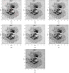 |
Fig. 3. Source images and restored images by various methods on one of the first testing set. The size of images is 1792 × 1792. The sub images of the top, middle, bottom red rectangles are shown in Fig. 4. (a) Image after AO correction. (b) SV-TVBD. (c) Retinal-CNN. (d) ED-DNN. (e) Recurrent-DNN. (f) CSSTN. (g) Speckle reconstruction image. |
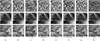 |
Fig. 4. Detailed results of the subregions (the area of red rectangles in the first from top to bottom in Fig. 3a). The (a) column is the worst source image. The (b) column is the best source image. The images of (c) to (h) column are restored by corresponding labeled methods. Image size is 256 × 256 with 8.832 arcsec × 8.832 arcsec. |
Evaluation on the first, second, and third testing sets in terms of average PSNR (dB).
To further evaluate the quality of the reconstruction of all methods, we calculate the contrast in the solar granulation, as shown in Table 4. Here, compared with the image after AO correction, the relative improvement of the contrast of the image restored by SV-TVBD, Retinal-CNN, ED-DNN, Recurrent-DNN, and our network are 35.71%, 69.25%, 8.38%, 13.35%, and 104.35%, respectively. This indicates that our method achieves the best contrast improvement with a clear appearance in this area. The contrast of image restored by our method is slightly lower than the speckle reconstruction image. In our experiments, our network consistently performs the best and restores much clearer images in terms of the granulation, sunspots, and penumbra subregions.
Contrast and the relative improvement of the contrast of granulation subregion on an image of the first testing set.
Since the deep learning networks we compare here are all spatially invariant, we also directly reconstruct small patches instead of whole images in order to carry out a fair comparison, as shown in Fig. 5. The region (indicated by the red arrow) of a small patch reconstructed by Retinal-CNN has severe stripe artifact. The region (indicated by the red arrow) cropped from the whole image that is reconstructed by ED-DNN and Recurrent-DNN show more detail than the one done directly via small patch recovery. The result of small patch reconstruction from our proposed method is almost the same as the result of small patches cropped by the result of the whole image reconstruction in terms of appearance.
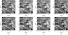 |
Fig. 5. Source images and restored images via various methods on one sample of the first testing set. The first row is the result of small patches clipped from restored the large images. The second row is the result of directly restoring the small patches. The images of (a) to (d) column are restored by correspondingly labeled methods. The regions marked by red arrows show some differences in the same method. The size of images is 256 × 256. (a) Retinal-CNN. (b) ED-DNN. (c) Recurrent-DNN. (d) CSSTN. |
Figure 6 shows images evaluated all methods on one image of the second testing set. As shown, SV-TVBD is nearly incapable of restoring the image details. In the three compared deep learning methods, ED-DNN and Recurrent-DNN still retain some blur effects; whereas Retinal-CNN shows sharper results than the other two methods. The structures in image restored by our proposed method are almost as same as the target speckle construction image. As seen in Table 3, the average PSNR among the whole second set of testing images recovered from our network is 4.18 dB, 7.89 dB, and 8.49 dB higher than that of the Retinal-CNN, ED-DNN, Recurrent-DNN, respectively.
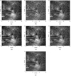 |
Fig. 6. Source images and restored images by various methods on one of the second testing set. The image size is 512 × 512. (a) Image after AO correction. (b) SV-TVBD. (c) Retinal-CNN. (d) ED-DNN. (e) Recurrent-DNN. (f) CSSTN. (g) Speckle reconstruction image. |
In order to better verify the generalization performance of our proposed method, we also evaluated all methods on the third testing set, which is composed of 656 nm band short exposure images with 10 ms exposure time of active region NOAA 12599 observed around the time [UT] 5:35:55, October 7, 2016 by NVST with an angular pixel size of 130 milliarcsec. As seen in Fig. 7, the improvement is shown to be very limited in the restored images by SV-TVBD, Retinal-CNN, ED-DNN, and Recurrent-DNN in comparison to the original images after AO correction. Our method can restore a sharper image and greater detail as compared to other methods.
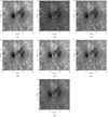 |
Fig. 7. Source images and restored images by various methods on one of the third testing set. The image size is 512 × 512. (a) Image after AO correction. (b) SV-TVBD. (c) Retinal-CNN. (d) ED-DNN. (e) Recurrent-DNN. (f) CSSTN. (g) Speckle reconstruction image. |
In order to better verify the generalization performance, we also evaluated all methods based on the fourth testing set without speckle reconstruction, which is made up of TiO band short exposure images with 1.8 ms exposure time of active region NOAA 12529 observed around the time [UT] 5:34:35, April 16, 2016 by NVST, with an angular pixel size of 34.5 milliarcsec. In photospheric restoring experiments, we found that the model trained with only photospheric data is better than the one trained with binding photospheric data and chromospheric data. The results restored by all methods trained only with photospheric data are shown in Fig. 8. We also show the restoration results of three different subregions in Fig. 9, corresponding to the three red rectangle areas in Fig. 8a, respectively. As seen in Fig. 9, the restored images by SV-TVBD have severe artifacts and the improvement is seen to be very limited in the restored images using Retinal-CNN, ED-DNN, and Recurrent-DNN than the original image after AO correction. The ED-DNN method has some high-value spots, as shown in Fig. 8d. Our method can restore sharper image and more details compared with other methods. As shown in Table 5, compared with the image after AO correction, the relative improvement of the contrast of granulation subregion image restored by SV-TVBD, Retinal-CNN, ED-DNN, Recurrent-DNN, and our network are 38.05%, 25.25%, 10.77%, 37.71%, and 49.83%, respectively.
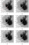 |
Fig. 8. Source images and restored images on one of the 4th testing set. The image size is 1792 × 1792. The results of the top, middle, bottom red rectangles are shown in Fig. 9. (a) Image after AO correction. (b) SV-TVBD. (c) Retinal-CNN. (d) ED-DNN. (e) Recurrent-DNN. (f) CSSTN. |
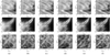 |
Fig. 9. Detailed results for the subregions (the area of red rectangle in the first from top to bottom in Fig. 8a). The first column is the source image. The images of (b) to (f) column are restored by correspondingly labeled methods. The image size is 256 × 256. (a) AO colsed-loop. (b) SV-TVBD. (c) Retinal-CNN. (d) Encoder-DNN. (e) Recurrent-DNN. (f) CSSTN. |
Contrast and the relative improvement of the contrast of granulation subregion on one image of the fourth testing set.
3.3. Ablation experiment
In this section, we conduct a number of ablation experiments, with all the results obtained with the model trained only on photospheric data.
3.3.1. Effectiveness of the size of channel sharing adaptive filters
To further investigate the proposed network, we experiment with channel sharing adaptive filters (spatially variant inter-frame filter, Fsvi, or spatially variant current-frame filter, Fsvc, in Fig. 1b) of different sizes in only TiO band image training. As seen in Table 6, this network has an adaptive filter size of 3 and a higher average PSNR than the network with an adaptive filter size of 5 with an average PSNR on the first set of test images. Therefore, we chose the size of the channel sharing filter as 3 (k is 3 in Fig. 1b) in our network. The proposed network has a smaller model size, thus, it is able to reconstruct an image with size of 1792 × 1792 faster.
Results of different sizes of channel sharing adaptive filters on the first testing set.
3.3.2. Effectiveness of channel sharing for adaptive filters
In order to validate the effectiveness of channel sharing for adaptive filters, we compare our network with a variant that changes the filter shared by the channel into a different filter for each channel (the number of generated filter channels changed from k2 to 128 × k2) in Fig. 1b. According to our results (shown in Table 7), the variant of proposed network has 0.34% performance improvement, while the network parameters is 44.20% more than the proposed network. Therefore, the network we propose in this paper achieves a balance between the computational complexity, model size, and performance.
Effectiveness of channel sharing for adaptive filters on the first testing set.
3.3.3. Effectiveness of perceptual loss
In order to validate the effectiveness of perceptual loss, we compare our network and a variant only trained with MSE loss. As seen in Fig. 10, the network trained combining with perceptual loss can obtain more clear images than those only using MSE loss.
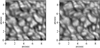 |
Fig. 10. Results using different losses. Left: restored result of network trained by MSE loss only. Right: restored result of our proposed method. The image size is 256 × 256. |
4. Conclusions and future work
In this work, we were able to achieve a blind restoration of solar images using an end-to-end channel sharing spatio-temporal network (CSSTN). The CSSTFAN sub-network can dynamically generate spatially variant filters from inputs, and together with the CSFAC layer, the proposed network can perform inter-frame and current-frame adjustments in the feature domain. Once the network is trained, it can work on images of any number of frames and any size.
We demonstrate that our proposed method can restore clearer and more detailed images compared with the several existing AO image deconvolution methods that are based on deep learning and traditional methods. Because the mixed loss function combining mean square error loss and perceptual loss is used during training, the images restored by our method have more textural details and are more realistic. We further demonstrate that the proposed method is not only capable of effectively removing the spatially variant blur included in training, but also of effectively removing the unseen spatially variant blur, indicating our network has an improved generalization performance. In addition, our method can obtain results that are comparable to the speckle reconstruction image. On the contrary, Retinal-CNN produces an artificial sharp edge in our data sets, perhaps because its network is too simple and only uses MSE loss, leading to its mimic training clear images almost only at the pixel level. We also found Recurrent-DNN to have nearly the same performance as ED-DNN in (Asensio Ramos et al. 2018). It is true that the performance of ED-DNN and Recurrent-DNN recovery is almost the same with regard to restoring our images based on models that have been made available to the community.
Since we applied the generated filter to the feature domain instead of directly to the image, a smaller filter size can be used to restore a clear image. Using the channel sharing inter-frame filters and current-frame filters, we can restore nearly the same clear latent image as the non-channel sharing variant of our network and with faster inference phase due to smaller model size. This may be because the limitation of positive bandwidth of the telescope (about 3) after two up-sampling rounds in CSSTN. The experimental results have demonstrated the effectiveness of the proposed method in terms of accuracy and inference speed. Zhou et al. (2019) have demonstrated that Falign can align features of current frame and previous frame by applying the FAC layer and Fdeblur can remove blur in the feature domain in their Fig. 7. The Fsvi and Fsvc are same as the Falign and Fdeblur in STFAN (Zhou et al. 2019). The STFAN method only explains alignment and deblurring filters at the visual and instinctive way for rigid motion (Zhou et al. 2019), but there is no complete theoretical explanation given there. In fact, Falign and Fdeblur are the output of feature layers of the neural network for triplet images (blurry and restored image of the previous time step and the current blurry image). The alignment and deblurring information are implied among these images: Falign is convolved with features of the previous time step, thus, it handles some adjustment of the inter-frame, which has some effects overlapping with alignment; Fdeblur is convolved with features of the current time step, thus it handles some adjustment of current frame which has some effects overlapping with deblurring. However, it is not fully certain that two adaptive filters are exactly in alignment and effectively deblurring. During our experiments, features convolved with Fsvc are seen to be sharper than features that come before the CSFAC layer, which may due to the inclusion of deblurring in the adjustment. However, features convolved with Fsvi do not see the alignment effect in comparison to features before the CSFAC layer, which maybe because of our image characters.
Although the binding two-band data trained network produces rather good results, it may be shown to have reduced performance in the individual band data compared to the individual band data-trained network. We think there are two reasons. Firstly, the diversity and quantity of training data can not be fully guaranteed, thus, there may be overfitting as a result. Secondly, training with two band data may make the network learn two different functions due to differences between photospheric (705 nm) and chromosphere (656 nm) data in telescope AO closed-loop imaging process. The differences at least include the following aspects: (1) the AO closed-loop residual error has different degrees of influence on image quality in 705 nm and 656 nm data; (2) the 705 nm data are over-sampling, but the 656 nm data are under-sampling; (3) the 656 nm data have gone through the narrow band filter, which has static optical phase difference, but the 705 nm data do not have that filter.
Based on the above hardware conditions with GPU, our network is currently capable to restore the 1792 × 1792 size image about in a half second in standard Pytorch1.0.0 environment without any particular optimization. It should not be a very hard that our method can restore current size images in several times faster heading to the real time AO image deconvolution with the special code optimization, rapid improvement of hardware performance and the improvement of network structure. Furthermore, since our proposed method is space variant blind restoring network independently from AO hardware and image size, CSSTN may also work on the AO images produced by other solar telescopes.
Of course, the proposed end-to-end neural network method has some limits. First, since the proposed method generates a spatially variant inter-frame filter and a spatially variant current-frame filter, it significantly increases the memory requirement than spatially invariant methods. An improved solution consists of explicitly aligning the previous frame and the current frame using the some sophisticated non-rigid image alignment methods, instead of implicitly generating a spatially variant inter-frame filter. If it is realized, the model size can be reduced; and on the other hand, the quality of restoration can be improved when the alignment loss is added to the loss function for the supervised learning. Second, we notice that training the network for blind deconvolution of multi-frame images can be done using synthetic data. To this end, we can generate synthetic images from existing solar-atmospheric magnetohydrodynamic simulations and use synthetic artificial wavefronts in the turbulent atmosphere to perturb them. These synthetic data can be used to interpret Fsvi and Fsvc as tip-tilt and blurring PSFs which helps better understanding network behavior. It might be interesting to using the local tip-tilt and high-order aberrations explicitly to restoration such as the good idea using network-embedded Zernike coefficients in (Asensio Ramos & Olspert 2021). With synthetic data and better interpretation, the ground truth and clear images can be obtained without using speckle image reconstruction algorithms, which helps to focus on improving the AO image deblurring method based on deep learning. In a future work, we will improve our work in order to rectify these these shortcomings.
The code for the networks using PyTorch can be downloaded from https://github.com/ShuaiWangUESTC/CSSTN
Acknowledgments
This work is partly supported by National Natural Science Foundation of China (NSFC) number 11703029, 11727805, 11733005, and the special science foundation of Quzhou, 2020D008.
References
- Al, N., Bendlin, C., Hirzberger, J., Kneer, F., & Bueno, J. T. 2004, A&A, 418, 1131 [NASA ADS] [CrossRef] [EDP Sciences] [Google Scholar]
- Armstrong, J. A., & Fletcher, L. 2021, MNRAS, 501, 2647 [CrossRef] [Google Scholar]
- Asensio Ramos, A., & Olspert, N. 2021, A&A, 646, A100 [CrossRef] [EDP Sciences] [Google Scholar]
- Asensio Ramos, A., Requerey, I., & Vitas, N. 2017, A&A, 604, A11 [NASA ADS] [CrossRef] [EDP Sciences] [Google Scholar]
- Asensio Ramos, A., de la Cruz Rodríguez, J., & Yabar, A. P. 2018, A&A, 620, A73 [NASA ADS] [CrossRef] [EDP Sciences] [Google Scholar]
- Ayers, G., & Dainty, J. C. 1988, Opt. Lett., 13, 547 [NASA ADS] [CrossRef] [PubMed] [Google Scholar]
- Babcock, H. W. 1953, PASP, 65, 229 [NASA ADS] [CrossRef] [Google Scholar]
- Berger, T. E., Loéfdahl, M. G., Shine, R. S., et al. 1998, ApJ, 495, 973 [NASA ADS] [CrossRef] [Google Scholar]
- Campisi, P., & Egiazarian, K. 2017, Blind Image Deconvolution: Theory and Applications (Boca Raton: CRC Press) [CrossRef] [Google Scholar]
- Chan, T. F., & Wong, C.-K. 1998, IEEE Trans. Image Process., 7, 370 [CrossRef] [Google Scholar]
- De Boer, C., Kneer, F., & Nesis, A. 1992, A&A, 257, L4 [Google Scholar]
- Denker, C., Yang, G., & Wang, H. 2001, Sol. Phys., 202, 63 [NASA ADS] [CrossRef] [Google Scholar]
- Denker, C., Mascarinas, D., Xu, Y., et al. 2005, Sol. Phys., 227, 217 [NASA ADS] [CrossRef] [Google Scholar]
- Diaz Baso, C. J., & Asensio Ramos, A. 2018, A&A, 614, A5 [NASA ADS] [CrossRef] [EDP Sciences] [Google Scholar]
- Diaz Baso, C. J., de la Cruz Rodriguez, J., & Danilovic, S. 2019, A&A, 629, A99 [CrossRef] [EDP Sciences] [Google Scholar]
- Ellerbroek, B., Britton, M., Dekany, R., et al. 2005, Int. Soc. Opt. Photon., 5903, 590304 [Google Scholar]
- Gonsalves, R. A. 1982, Opt. Eng., 21, 215829 [NASA ADS] [CrossRef] [Google Scholar]
- Gravet, R., Cabrera-Vives, G., Pérez-González, P. G., et al. 2015, ApJS, 221, 8 [NASA ADS] [CrossRef] [Google Scholar]
- He, K., Zhang, X., Ren, S., & Sun, J. 2015, Proceedings of the IEEE International Conference on Computer Vision, 1026 [Google Scholar]
- He, K., Zhang, X., Ren, S., & Sun, J. 2016, Proceedings of the IEEE Conference on Computer Vision and Pattern Recognition, 770 [Google Scholar]
- Holmes, T. J. 1992, J. Opt. Soc. Am. A, 9, 1052 [NASA ADS] [CrossRef] [Google Scholar]
- Janßen, K., Vögler, A., & Kneer, F. 2003, A&A, 409, 1127 [NASA ADS] [CrossRef] [EDP Sciences] [Google Scholar]
- Jia, X., De Brabandere, B., Tuytelaars, T., & Gool, L. V. 2016, Adv. Neural Inf. Process. Syst., 29, 667 [Google Scholar]
- Jiang, W., Huang, S., Ling, N., & Wu, X. 1989, Int. Soc. Opt. Photon., 965, 266 [Google Scholar]
- Johns, M., McCarthy, P., Raybould, K., et al. 2012, Int. Soc. Opt. Photon., 8444, 84441H [Google Scholar]
- Johnson, J., Alahi, A., & Fei-Fei, L. 2016, European Conference on Computer Vision (Springer), 694 [Google Scholar]
- Keller, C., & Von Der Luehe, O. 1992, A&A, 261, 321 [Google Scholar]
- Kingma, P. D., & Ba, L. J. 2015, International Conference on Learning Representations, ICLR 2015, San Diego [Google Scholar]
- Kong, L., Zhang, L., Zhu, L., et al. 2016, Chin. Opt. Lett., 14, 100102 [CrossRef] [Google Scholar]
- Kong, L., Zhu, L., Zhang, L., Bao, H., & Rao, C. 2017, IEEE Photon. J., 9, 1 [Google Scholar]
- Krishnan, D., Tay, T., & Fergus, R. 2011, Blind Deconvolution Using a Normalized Sparsity Measure, CVPR 2011 (IEEE), 233 [Google Scholar]
- Lane, R. G. 1992, J. Opt. Soc. Am. A, 9, 1508 [NASA ADS] [CrossRef] [Google Scholar]
- Levin, A., Weiss, Y., Durand, F., & Freeman, W. T. 2011, Efficient Marginal Likelihood Optimization in Blind Deconvolution, CVPR 2011 (IEEE), 2657 [Google Scholar]
- Liang, J., Williams, D. R., & Miller, D. T. 1997, J. Opt. Soc. Am. A, 14, 2884 [CrossRef] [Google Scholar]
- Löfdahl, M. G. 2002, Int. Soc. Opt. Photon., 4792, 146 [Google Scholar]
- Löfdahl, M. G., & Scharmer, G. 1994, A&AS, 107, 243 [Google Scholar]
- Löfdahl, M., Kiselman, D., & Scharmer, G. 2004, A&A, 414, 717 [NASA ADS] [CrossRef] [EDP Sciences] [Google Scholar]
- Maas, A. L., Hannun, A. Y., & Ng, A. Y. 2013, Proc. ICML, 30, 3 [Google Scholar]
- Mao, X. J., Shen, C., & Yang, Y. B. 2016, Advances in Neural Information Processing Systems 29 (NIPS 2016), 2810 [Google Scholar]
- Mildenhall, B., Barron, J. T., Chen, J., et al. 2018, Proceedings of the IEEE Conference on Computer Vision and Pattern Recognition, 2502 [Google Scholar]
- Molina, R., Mateos, J., & Katsaggelos, A. K. 2006, IEEE Trans. Image Process., 15, 3715 [NASA ADS] [CrossRef] [Google Scholar]
- Paszke, A., Gross, S., Massa, F., et al. 2019, Advances in Neural Information Processing Systems, 8026 [Google Scholar]
- Paxman, R. G., Schulz, T. J., & Fienup, J. R. 1992, J. Opt. Soc. Am. A, 9, 1072 [NASA ADS] [CrossRef] [Google Scholar]
- Perrone, D., & Favaro, P. 2014, Proceedings of the IEEE Conference on Computer Vision and Pattern Recognition, 2909 [Google Scholar]
- Rao, C.-H., Jiang, W.-H., Fang, C., et al. 2003, Chin. J. Astron. Astrophys., 3, 576 [CrossRef] [Google Scholar]
- Rao, C., Zhu, L., Rao, X., et al. 2015, Chin. Opt. Lett., 13, 120101 [CrossRef] [Google Scholar]
- Rao, C., Zhu, L., Rao, X., et al. 2016, ApJ, 833, 210 [CrossRef] [Google Scholar]
- Rao, C., Gu, N., Rao, X., et al. 2020, First Light of the 1.8-m Solar Telescope–CLST (Springer) [Google Scholar]
- Rimmele, T. R. 2000, Int. Soc. Opt. Photon., 4007, 218 [Google Scholar]
- Roorda, A., & Williams, D. R. 1999, Nature, 397, 520 [CrossRef] [Google Scholar]
- Rousset, G., Fontanella, J., Kern, P., Gigan, P., & Rigaut, F. 1990, A&A, 230, L29 [Google Scholar]
- Scharmer, G. B., Shand, M., Lofdahl, M. G., Dettori, P. M., & Wei, W. 2000, Int. Soc. Opt. Photon., 4007, 239 [Google Scholar]
- Scharmer, G. B., Gudiksen, B. V., Kiselman, D., Löfdahl, M. G., & van der Voort, L. H. R. 2002, Nature, 420, 151 [NASA ADS] [CrossRef] [PubMed] [Google Scholar]
- Schulz, T. J. 1993, J. Opt. Soc. Am. A, 10, 1064 [NASA ADS] [CrossRef] [Google Scholar]
- Sidky, E. Y., & Pan, X. 2008, Phys. Med. Biol., 53, 4777 [CrossRef] [PubMed] [Google Scholar]
- Sütterlin, P., Rubio, L. B., & Schlichenmaier, R. 2004, A&A, 424, 1049 [NASA ADS] [CrossRef] [EDP Sciences] [Google Scholar]
- Thiébaut, E., & Conan, J.-M. 1995, J. Opt. Soc. Am. A, 12, 485 [NASA ADS] [CrossRef] [Google Scholar]
- Tritschler, A., & Schmidt, W. 2002, A&A, 388, 1048 [NASA ADS] [CrossRef] [EDP Sciences] [Google Scholar]
- Tsumuraya, F., Miura, N., & Baba, N. 1994, A&A, 282, 699 [NASA ADS] [Google Scholar]
- Van Noort, M., Van Der Voort, L. R., & Löfdahl, M. G. 2005, Sol. Phys., 228, 191 [NASA ADS] [CrossRef] [Google Scholar]
- Von der Luehe, O. 1994, A&A, 281, 889 [Google Scholar]
- Von der Lühe, O. 1993, A&A, 268, 374 [Google Scholar]
- Wenhan, J., Yudong, Z., Changhui, R., et al. 2011, Acta Opt. Sin., 31, 0900106 [CrossRef] [Google Scholar]
- Xiao, F., Zhao, J., Zhao, H., Dai, Y., & Zhang, Y. 2017, Biomed. Opt. Exp., 8, 5675 [CrossRef] [Google Scholar]
- Yu, T., Chang-hui, R., & Kai, W. 2009, Chin. Astron. Astrophys., 33, 223 [CrossRef] [Google Scholar]
- Zhang, P., Yang, C., Xu, Z., et al. 2017, Sci. Rep., 7, 1 [CrossRef] [Google Scholar]
- Zhong, L., Tian, Y., & Rao, C. 2014, Opt. Exp., 22, 29249 [NASA ADS] [CrossRef] [Google Scholar]
- Zhou, S., Zhang, J., Pan, J., et al. 2019, Proceedings of the IEEE International Conference on Computer Vision, 2482 [Google Scholar]
All Tables
Architecture of channel sharing spatio-temporal filter adaptive network (CSSTFAN) sub-network.
Evaluation on the first, second, and third testing sets in terms of average PSNR (dB).
Contrast and the relative improvement of the contrast of granulation subregion on an image of the first testing set.
Contrast and the relative improvement of the contrast of granulation subregion on one image of the fourth testing set.
Results of different sizes of channel sharing adaptive filters on the first testing set.
All Figures
|
Fig. 1. Proposed deep neural network architecture. Panel a: shows our proposed channel sharing spatio-temporal network (CSSTN). Panel b: is a channel sharing spatio-temporal filter adaptive network (CSSTFAN) sub-network. Panel c: is the meaning of different color blocks and symbols in the network. CSSTN consists of three sub-networks: a feature extraction network, a CSSTFAN, and a reconstruction network. Firstly the feature extraction network extracts features Et from the current blurry image Bt. Given the blurred image Bt − 1 and restored image Rt − 1 of the previous time step, and current input image Bt, the CSSTFAN generates the Fsvi and Fsvc in order. Using CSFAC layer ⊛, CSSTFAN convolves Fsvi with features Ht − 1 of the previous time step and convolves Fsvc with features Et. Finally, the reconstruction network restores the latent image from the fused features Ct. k denotes the filter size of CSFAC layer and it is 3 in our final network. |
| In the text | |
|
Fig. 2. Proposed channel sharing filter adaptive convolutional layer (CSFAC). The generated filter F is h × w × k2. We reshape it to h × w × k × k, and then apply the filter to each channel of the feature Q, finally get transformed feature |
| In the text | |
|
Fig. 3. Source images and restored images by various methods on one of the first testing set. The size of images is 1792 × 1792. The sub images of the top, middle, bottom red rectangles are shown in Fig. 4. (a) Image after AO correction. (b) SV-TVBD. (c) Retinal-CNN. (d) ED-DNN. (e) Recurrent-DNN. (f) CSSTN. (g) Speckle reconstruction image. |
| In the text | |
|
Fig. 4. Detailed results of the subregions (the area of red rectangles in the first from top to bottom in Fig. 3a). The (a) column is the worst source image. The (b) column is the best source image. The images of (c) to (h) column are restored by corresponding labeled methods. Image size is 256 × 256 with 8.832 arcsec × 8.832 arcsec. |
| In the text | |
|
Fig. 5. Source images and restored images via various methods on one sample of the first testing set. The first row is the result of small patches clipped from restored the large images. The second row is the result of directly restoring the small patches. The images of (a) to (d) column are restored by correspondingly labeled methods. The regions marked by red arrows show some differences in the same method. The size of images is 256 × 256. (a) Retinal-CNN. (b) ED-DNN. (c) Recurrent-DNN. (d) CSSTN. |
| In the text | |
|
Fig. 6. Source images and restored images by various methods on one of the second testing set. The image size is 512 × 512. (a) Image after AO correction. (b) SV-TVBD. (c) Retinal-CNN. (d) ED-DNN. (e) Recurrent-DNN. (f) CSSTN. (g) Speckle reconstruction image. |
| In the text | |
|
Fig. 7. Source images and restored images by various methods on one of the third testing set. The image size is 512 × 512. (a) Image after AO correction. (b) SV-TVBD. (c) Retinal-CNN. (d) ED-DNN. (e) Recurrent-DNN. (f) CSSTN. (g) Speckle reconstruction image. |
| In the text | |
|
Fig. 8. Source images and restored images on one of the 4th testing set. The image size is 1792 × 1792. The results of the top, middle, bottom red rectangles are shown in Fig. 9. (a) Image after AO correction. (b) SV-TVBD. (c) Retinal-CNN. (d) ED-DNN. (e) Recurrent-DNN. (f) CSSTN. |
| In the text | |
|
Fig. 9. Detailed results for the subregions (the area of red rectangle in the first from top to bottom in Fig. 8a). The first column is the source image. The images of (b) to (f) column are restored by correspondingly labeled methods. The image size is 256 × 256. (a) AO colsed-loop. (b) SV-TVBD. (c) Retinal-CNN. (d) Encoder-DNN. (e) Recurrent-DNN. (f) CSSTN. |
| In the text | |
|
Fig. 10. Results using different losses. Left: restored result of network trained by MSE loss only. Right: restored result of our proposed method. The image size is 256 × 256. |
| In the text | |
Current usage metrics show cumulative count of Article Views (full-text article views including HTML views, PDF and ePub downloads, according to the available data) and Abstracts Views on Vision4Press platform.
Data correspond to usage on the plateform after 2015. The current usage metrics is available 48-96 hours after online publication and is updated daily on week days.
Initial download of the metrics may take a while.