| Issue |
A&A
Volume 674, June 2023
|
|
|---|---|---|
| Article Number | A126 | |
| Number of page(s) | 15 | |
| Section | Astronomical instrumentation | |
| DOI | https://doi.org/10.1051/0004-6361/202244904 | |
| Published online | 13 June 2023 | |
Cascaded Temporal and Spatial Attention Network for solar adaptive optics image restoration
1
University of Electronic Science and Technology of China,
Xiyuan Avenue, West Hi-tech Zone, Chengdu,
Sichuan
611731, PR China
e-mail: This email address is being protected from spambots. You need JavaScript enabled to view it.
2
Yangtze Delta Region Institute of University of Electronic Science and Technology of China,
Chengdian Road, Kecheng, Quzhou,
Zhejiang
324003, PR China
3
Institute of Optics and Electronics Chinese Academy of Sciences,
Box 350,
Shuangliu, Chengdu,
Sichuan
610209, PR China
e-mail: This email address is being protected from spambots. You need JavaScript enabled to view it.
4
University of Chinese Academy of Sciences,
Yanqi Lake East Road, Huairou,
Beijing
100049, PR China
5
Key Laboratory on Adaptive Optics, Chinese Academy of Sciences,
Box 350,
Shuangliu, Chengdu,
Sichuan
610209, PR China
Received:
7
September
2022
Accepted:
13
March
2023
Abstract
Context. Atmospheric turbulence severely degrades the quality of images observed through a ground-based telescope. An adaptive optics (AO) system only partially improves the image quality by correcting certain level wavefronts, making post-facto image processing necessary. Several deep learning-based methods have recently been applied in solar AO image post-processing. However, further research is still needed to get better images while enhancing model robustness and using inter-frame and intra-frame information.
Aims. We propose an end-to-end network that can better handle solar adaptive image anisoplanatism by leveraging attention mechanisms, pixel-wise filters, and cascaded architecture.
Methods. We developed a cascaded attention-based deep neural network named Cascaded Temporal and Spatial Attention Network (CTSAN) for solar AO image restoration. CTSAN consists of four modules: optical flow estimation PWC-Net for inter-frame explicit alignment, temporal and spatial attention for dynamic feature fusion, temporal sharpness prior for sharp feature extraction, and encoder-decoder architecture for feature reconstruction. We also used a hard example mining strategy to create a loss function in order to focus on the regions that are difficult to restore, and a cascaded architecture to further improve model stability.
Results. CTSAN and the other two state-of-the-art (SOTA) supervised learning methods for solar AO image restoration are trained on real 705 nm photospheric and 656 nm chromospheric AO images supervised by corresponding Speckle images. Then all the methods are quantitatively and qualitatively evaluated on five real testing sets. Compared to the other two SOTA methods, CTSAN can restore clearer solar images, and shows better stability and generalization performance when restoring the lowest contrast AO image.
Key words: methods: data analysis / Sun: photosphere / techniques: image processing
Authors contributed equally.
Corresponding author.
© The Authors 2023
 Open Access article, published by EDP Sciences, under the terms of the Creative Commons Attribution License (https://creativecommons.org/licenses/by/4.0), which permits unrestricted use, distribution, and reproduction in any medium, provided the original work is properly cited.
This article is published in open access under the Subscribe to Open model. This email address is being protected from spambots. You need JavaScript enabled to view it. to support open access publication.
1 Introduction
Large and advanced telescopes are usually built on the ground due to frequent forefront technology updating and maintenance (Asensio Ramos & Olspert 2021). Observing with ground-based telescope introduces perturbations because the light inevitably comes through the Earth’s atmosphere. The random fluctuation caused by the atmospheric turbulence leads to the wavefront distortion of light waves, which severely degrades optical system imaging quality (Lukin et al. 2020), especially in solar observation due to daytime stronger atmosphere turbulence. Adaptive optics (AO) is one of the most effective ways to overcome atmospheric turbulence; it consists of a wavefront detector, corrector, and controller (Hinnen et al. 2008; Haffert et al. 2022). The core idea of AO is to measure the optical wave-front distortion and compensate it in real time to solve the dynamic interference caused by atmospheric turbulence (Jiang 2018). Currently, AO has been widely applied in various fields, including ground-based observation (Rousset et al. 1990), high-resolution imaging of ground-based telescopes (Rao et al. 2003), space optical remote sensing (Armstrong & Fletcher 2021), high-energy laser transmission (Baranec et al. 2014), optical communication technology (Weyrauch et al. 2002), laser processing applications (Salter & Booth 2019), and ophthalmology (Liang et al. 1997). However, AO can only partially compensate the wavefront due to the hardware limitations, such as insufficient sensor accuracy and a fixed number of correction modes (Rao et al. 2016a, Rao et al. 2018, 2020; Rimmele & Marino 2011). These limitations make post-facto image processing for AO closed-loop images necessary and crucial, especially for a telescope with a large field of view (FoV, Asensio Ramos et al. 2018; Asensio Ramos & Olspert 2021).
Currently, three traditional post-processing methods are applied in the AO image area, the speckle imaging (Speckle), phase diversity (PD), and deconvolution methods (Bao et al. 2018). The Speckle method has achieved good results based on reconstructing the phase and amplitude of objects by employing statistical characteristics of atmospheric turbulence (Keller & Von Der Luehe 1992; Stachnik et al. 1977; Zhong et al. 2020). However, it requires numerous short-exposure degraded frames with no significant change during the imaging process. These requirements cause a large amount of data processing and time-consuming computing, thus leading to some restrictions in practical application (Codona & Kenworthy 2013). The PD algorithm normally employs paired focus-defocus images to establish a constrained metric to restore the target images and its wavefront information simultaneously (Carbillet et al. 2006; Blanc et al. 2003). One of the successful PD algorithms is MOMFBD (van Noort et al. 2006). The main shortcomings of PD reside in its extra hardware and large computational requirement (Asensio Ramos & Olspert 2021). The deconvolu-tion method can be divided into deconvolution with wavefront sensing (DWFS, Restaino 1992; Rao & Jiang 2002) and blind deconvolution (BD, Tian et al. 2008; Asensio Ramos et al. 2018). The DWFS algorithms employ wavefront information detected by wavefront sensors, combined with short-exposure images simultaneously (Welsh & Roggemann 1995). However, it is not real-time and highly susceptible to noise. The BD algorithm only uses degraded images to estimate the target and point spread function representing the wavefront disturbance, but directly solving BD is seriously ill-posed. So BD algorithms focus on finding proper constraint information to get better solutions and converge behavior (Wang et al. 2023).
With the improvement of computing power and the algorithm theory innovation, deep learning has made significant advances in various fields, including computer vision (Voulodimos et al. 2018), signal processing (Ye et al. 2021), natural language processing (Vaswani et al. 2017), network science (He et al. 2021), life science (Zhang et al. 2021), and clinical detection (Jiang et al. 2022). In image and video high-quality reconstruction, deep learning is also successfully used to defect correction (Ratnasingam 2019), video inpainting (Zou et al. 2021), deblurring (Pan et al. 2020), and denoising (Tian et al. 2020). Wang et al. (2019) employed a deformable convolution module with pyramid architecture for frame alignment and a temporal and spatial attention fusion module followed by a reconstruction module to restore high-resolution videos (Zhang et al. 2022). Pan et al. (2020) construct a deep network named cascaded deep video deblurring using a temporal sharpness prior to deblurring on real challenging videos; it first aligns adjacent frames, then computes the sharpness prior, and finally feeds both the blurry images and the prior into an encoder-decoder network.
Deep learning-based methods are also used in solar image restoration and AO image post-processing (Guo et al. 2022; Jia et al. 2019). Baso et al. (2019) designed a neural network with autoencoder architecture to denoise solar images corrupted by complicated noise corruption such as instrumental artifacts and nonlinear post-processing. Fei et al. (2017) constructed an end-to-end network to learn the mapping between the blurred and sharp AO retinal images, which are subsequently applied to restore real solar AO images (Wang et al. 2021). Asensio Ramos et al. (2018) proposed two different deep convolutional neural networks for multi-frame blind deconvolution of the solar image. The first is an encoder-decoder deconvolution neural network (EDDNN) for restoring images from a fixed number of frames (Asensio Ramos et al. 2018). The second is a recurrent network with an encoder-decoder network using an arbitrary number of frames, which is more challenging to train than EDDNN due to the existence of recurrent connections (Asensio Ramos et al. 2018). Asensio Ramos & Olspert (2021) used an unsu-pervised neural network to restore the solar image and estimate the wavefronts at the same time. Based on the adaptive filter, Wang et al. (2021) proposed a blind restoration network (CSSTN) for solar AO image post-processing by constructing two sophisticated spatially variant adaptive filters for deblurring and aligning. CSSTN outperforms other deep learning-based solar image restoration methods in four real solar AO closed-loop datasets.
Although these deep learning models perform well in their datasets, model robustness be further considered in real solar AO imaging systems with unpredictable imaging conditions and complex observation scenes. Among these circumstances, the properties of images degraded by atmospheric turbulence should also be considered. And further research is still needed to enhance model robustness and for a better use of inter-frame and intra-frame information.
Aligning multiple frames using inter-frame information is essential for restoring multiple frames degraded by large motions, atmospheric disturbances, and large FoV blurs (Wang et al. 2019, 2021). Existing aligning methods can be divided into explicit and implicit branches (Chan et al. 2021). Implicit aligning has been applied in solar AO restoration, but its effectiveness in alignment needs to be verified (Wang et al. 2021). Some researchers have validated the better robustness of the explicit alignment model in various denoising and deblurring tasks (Otte & Nagel 1994; Ehret et al. 2019; Xiang et al. 2020). However, different adjacent frames are usually hard to fully and precisely align, and are not equally informative in the case of large blurring (Wang et al. 2019). The attention mechanism that emphasizes spatially and temporally important features to prevent the adverse effect of misalignment and unalignment arising from the preceding alignment stage has achieved great success and is validated in various visual tasks, including image reconstruction and video deblurring (He et al. 2022; Zamir et al. 2021).
We propose the Cascaded Temporal and Spatial Attention Network (CTSAN) based on the explicit alignment and attention mechanism. CTSAN is constructed with pixel-wise filters and attention mechanisms to better handle anisoplanatism in solar AO images (Wang et al. 2019; Pan et al. 2020). Our main contributions are: (1) an explicit alignment module to align adjacent frames at pixel-level with pre-training and fine-tuning strategy to increase training efficiency and model accuracy; (2) a temporal and spatial attention (TSA) module to construct pixel-wise filters and emphasize features temporally and spatially; (3) two modules to address uneven blurring; the temporal sharpness prior (TSP) module is introduced to increase the weights of clearer patches, while the hard example mining strategy (HEM) module lets the loss function concentrate on severely blurred regions to lead the model to focus on learning to produce better results; and (4) cascaded two-stage architectures to improve performance further and ensure model robustness with the same number of training parameters as one-stage architecture.
This article is divided into five sections. Section 1 briefly introduces the background, research status, and motivation. The remainder of this article is organized as follows. Section 2 details the principle and architecture of our proposed network. Section 3 describes the parameters of five real datasets, network training details, and hyperparameter settings. Section 4 shows the qualitative and quantitative evaluation results of all networks trained with two-band and single-band training sets and our model’s ablation experiments. Section 5 presents the discussion and our conclusions.
2 Cascaded temporal and spatial attention network
2.1 Network structure
Our proposed CTSAN is constructed by the multiple Temporal and Spatial Attention Network (TSAN), which consists of four parts: PWC-Net, TSA, TSP, and the feature reconstruction module, as shown in Fig. 1a. Each TSAN unit takes three consecutive frames as input, and outputs one restored image, as shown in Fig. 1b. CTSAN is built in a cascaded two-stage manner, which inputs five consecutive frames to restore one clear image, as shown in Fig. 1c. The architecture (including kernel size and depth), and input and output shapes of the reconstruction network are shown in Table 1. The properties of these super blocks numbered as Ci.j in Fig. 1a are shown in Table 1, while i, j refer to the superblock and the block inside the superblock (Asensio Ramos et al. 2018).
Dense optical flow can provide motion information by estimating the displacement field between two consecutive frames, which are able to generate higher resolution results (Fortun et al. 2015; Pan et al. 2020; Zou et al. 2021). PWC-Net is a compact and effective CNN model for dense optical flow estimation. Unlike the traditional optical flow estimation approach, PWC-Net employs a multi-scale feature pyramid, warping, and cost volumes, and performs better in real images with large motions and image edges corrupted by motion blur, atmospheric change, and noise (Sun et al. 2018; Gu et al. 2019). We use PWC-Net in our proposed network. Given three consecutive frames Ii–1, Ii and Ii+1 the optical flow using PWC-Net for alignment to frame Ii can be computed as follows:
 (1)
(1)
Here NO (·) denotes PWC-Net. ui+1→i· = (ui+1→i, υi+1→i) and ui−1→i = (ui−1→i, υi−1→i) denote backward flow and forward flow at frame Ii+1 and Ii_1, respectively; and u, υ are the velocity vectors of the optical flow along the X-axis and Y-axis, respectively (Hyun Kim & Mu Lee 2015; Meister et al. 2018; Maurer & Bruhn 2018).
According to the obtained optical flow ui+1→i and ui−1→i, we employ warping operation to align the corresponding adjacent frames to reference frame Ii (Lai et al. 2019):
 (2)
(2)
The x denotes every pixel location. We note that we estimate the optical flow from frame Ii+1 and Ii−1 to frame Ii instead of frame Ii to frame Ii−1 and Ii+1 because the warped results of optical flow ui→i+i and ui→i−i leads to blurred images (Pan et al. 2020).
The network architecture of the TSA fusion module is shown in Fig. 2. Temporal attention in TSA is designed to give more attention to the adjacent frame aligned better to Ii. We first compute the similarity distance of aligned frames Ii+1 (x + ui+1→i), Ii−1 (x + ui−1→i) to the reference frame Ii. The similarity distance (matrix of temporal attention map) of aligned frame Ii+1 (x + ui+1→i) is computed as
 (3)
(3)
where θ (Ii+1 (x + ui+1→i)) and ϕ (Ii (x)) are two embeddings computed by convolution filters, and the ⊗ is the dot product as shown in Fig. 2 (left). The Sigmoid function in Eq. (3) limits the output value of h in [0,1], which can stabilize gradient back-propagation (Wang et al. 2019); hi_1 is computed in a similar way. Then the temporal attention map is multiplied to the original aligned frame:
 (4)
(4)
Here ⊙ is the pixel-wise multiplication. After calculating the temporal attention map Ĩi_1 (x + ui_1→i·) in the same way, the fusion convolution layer is used to fuse these features:
![Mathematical equation: ${{\bf{f}}_{i,{\rm{conv}}}} = {\rm{Conv}}\left( {\left[ {{{{\bf{\tilde I}}}_{i + 1}}\left( {{\bf{x}} + {{\bf{u}}_{i + 1 \to i}}} \right),{{\bf{I}}_i}\left( {\bf{x}} \right),{{{\bf{\tilde I}}}_{i - 1}}\left( {{\bf{x}} + {{\bf{u}}_{i - 1 \to i}}} \right)} \right]} \right).$](/articles/aa/full_html/2023/06/aa44904-22/aa44904-22-eq5.png) (5)
(5)
The symbol [, ] denotes concatenation operation, and Conv represents the convolution filter corresponding to the “Fusion Conv” block in Fig. 2. Then ficonv is fed into the spatial attention part, which adaptively makes an impact on spatial pixels by employing spatial affine transformation (Wang et al. 2018, 2019). Assuming fi,TSA is the final output of the TSA module, the spatial attention operation is expressed as follows:
 (6)
(6)
The symbol ⊕ is an element-wise addition. The masks γi and βi, which have the same dimension as fi,conv and respectively correspond to the input of L5,5 and L5,6 in Table 2, are generated by spatial attention module with three-layer feature pyramid architecture that increases the attention receptive field (Wang et al. 2018, 2019). The layer inside the operation of spatial attention in TSA denoted as Li,j are shown in Table 2, while i refers to the layer number of pyramid architecture, corresponding to the number in the spatial attention part of Fig. 2, and j refers to the inside operation to get the corresponding ith layer. The yellow blocks in Fig. 2 are output features of each layer.
We use TSP to reconstruct the clear latent image by adding sharpness weights in feature map (Cho et al. 2012). The sharpness in TSP is formulated as
 (7)
(7)
where the parameter j is set to 1 and −1, and w(x) is an image patch centered at pixel x. The outputs of the TSP and TSA modules are finally concatenated and fed into the feature reconstruction network:
![Mathematical equation: ${{\bf{I}}_{i,r}} = {N_R}\left( {\left[ {{{\bf{f}}_{i,TSA}},{{\bf{C}}_i}\left( {\bf{x}} \right)} \right]} \right).$](/articles/aa/full_html/2023/06/aa44904-22/aa44904-22-eq8.png) (8)
(8)
Here NR (·) represents the feature reconstruction network, a standard encoder-decoder architecture with skip connection (Tao et al. 2018), and Ii,r is the final restored image of each TSAN unit, which corresponds to C6,4 in Table 1.
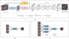 |
Fig. 1 Overview of proposed CTSAN architecture. Panel a shows the network detail of the TSAN unit. Panel b is the input and output of a single TSAN unit. Panel c shows the forward propagation process of CTSAN. The same trained TSAN parameter is used four times to construct the cascaded two-stage architecture. |
Architecture of feature reconstruction network.
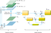 |
Fig. 2 Architecture of TSA module for feature fusion. The output feature of temporal attention is modulated by the fusion convolution block before feeding into the spatial attention module. |
2.2 Loss function
The common optimization goal of a restoring network is to minimize L1 norm between the restored latent image and referenced supervised image. However, purely using the L1 norm will lead to blurred edges and boundaries, producing artifacts in subsequent latent image restoration (Pan et al. 2020; Xu et al. 2019). We deal with this problem by adding a HEM module in the loss function to pay attention to severely blurred regions and subsequently lead the model to focus on learning to produce better results (Xu et al. 2019). Accordingly, the TSAN unit loss of frame Ii can be expressed as
 (9)
(9)
where T represents the TSAN unit, Ii,c corresponds to the ith clear frame restored by Speckle. The Mi is the HEM mask and is computed as follows:
 (10)
(10)
Here Mi,h is the hard sample mask representing the top a% (a є [0,100]) pixels in L1 loss value in descending order of current restored image pixel in training iteration. The mask Mi,r, which is used to enhance model robustness, represents the randomly selected b% (b є [0,100]) pixels of the current restored image pixel in training iteration. The λ in Eq. (9) is the HEM module weight parameter.
CTSAN is constructed by a cascaded multi-stage approach, which can improve model stability when the input image has complicated blurrings (Zhang et al. 2022). To balance accuracy and speed, we empirically set the stage number to 2, as shown in Fig. 1c. During the iteration of CTSAN training, the overall loss is calculated according to the forward propagation results of four TSAN units shown in Fig. 1c, which is correspondingly formulated as follows:
 (11)
(11)
The symbols T1 and T2 represent the TSAN units used in the first and second stages. In the first stage of CTSAN, the ℒi-1,T1, ℒi,T1, and ℒi+1,Tl are calculated from Ii_1,r, Ii,r and Ii+1,r, which are restored from raw AO images, as shown in Col. 1 of Fig. 1c. In the second stage of CTSAN, the ℒi,T2 is calculated from Ii,r, which is restored from the three outputs of the first stage, as shown in Col. 2 of Fig. 1c. Hence, the overall loss ℒi ensures that CTSAN is robust to different types of inputs. In each iteration’s backward propagation of CTSAN, a unique TSAN parameter set based on a single TSAN unit is updated for faster convergence and lower computational costs. At the next iteration’s forward propagation, the updated unique TSAN parameter will be used four times in constructing the cascaded architecture, sharing the same TSAN parameters in the first and second stages of CTSAN, as shown in Fig. 1c.
Architecture of spatial attention part in TSA Module with upsampling implemented by bilinear interpolation.
3 Dataset and training
3.1 Dataset
Five real short-exposure solar image datasets with AO closed-loop corrections are employed in our experiment, including three datasets of the photospheric 705 nm band and two datasets of the chromospheric 656 nm band. These solar images were observed by the New Vacuum Solars Telescope (NVST), a one-meter vacuum solar telescope located near Fuxian Lake, with a ground layer adaptive optics (GLAO) system or classical adaptive optics (CAO) system (Rao et al. 2015, 2016b; Kong et al. 2016, 2017). The dataset parameters are listed in Table 3, and the first three datasets are the same as the first three datasets used in CSSTN (Wang et al. 2021). The Speckle method uses 100 images to restore one Speckle image (Zhong et al. 2014). We define an AO closed-loop source image and its corresponding Speckle image as a pair. The first photosphere dataset is divided into 5200, 500, and 1000 pairs as the first training, validation, and testing set. The first chromosphere dataset is divided into 70, 10, and 20 pairs as the second training, validation, and testing set. To keep the balance between the two training sets, we duplicate the second training set 80 times to keep the balance and obtain 5600 pairs of images for the second training set, as shown in Table 3. The third, fourth, and fifth datasets are only used as testing sets.
3.2 Network training
Some research, such as Wang et al. (2021) and Asensio Ramos et al. (2018), have verified that Recurrent-DNN has nearly the same performance as EDDNN, which has a similar architecture with our encoder-decoder backbone structure. CSSTN is the latest solar AO image blind deconvolution method based on two adaptive filters, outperforming several previous supervised learning methods and TV-based blind deconvolution methods. Therefore, EDDNN and CSSTN are selected as comparison methods in this research.
For all methods, a single-band trained model is used to restore all TiO (750 nm) testing sets to restore better photospheric images (Wang et al. 2021), and a dual-band trained model is used to restore all chromospheric testing sets to prevent overflt-ting on our small chromospheric training sets. CSSTN is trained on a computer with an Intel i7-8700K CPU with 16GB memory and an NVIDIA 12GB Titan Xp GPU (Wang et al. 2021), while EDDNN and CTSAN are trained on a server with 2 Intel Xeon 4210R CPU, 128GB RAM, and NVIDIA 24GB RTX3090 with Ubuntu 20.04 OS. Data augmentation is employed in data preprocessing. Randomly rotating at 90 degrees and horizontally and vertically flipping are used. Then, the randomly cropped patch with 88 × 88 (Asensio Ramos et al. 2018), 256 × 256 (Wang et al. 2021), and 256 × 256 pixels are used to train EDDNN, CSSTN, and CTSAN, respectively.
CTSAN is implemented by the CUDA 11.7 and PyTorch 1.13.0 platform. PWC-Net of CTSAN is initialized by introducing its parameters pre-training on KITTI and Sintel benchmark datasets and fine-tuning on our training sets with learning rate 1 × 10⁻⁶ (Sun et al. 2018; Menze & Geiger 2015; Butler et al. 2012). KITTI contains static and dynamic scenes, large motion, severe illumination changes, and occlusions, while Sin-tel contains various strong atmospheric effects, defocus blur, and camera noise, among others (Sun et al. 2018; Menze & Geiger 2015; Butler et al. 2012). This pre-training strategy can efficiently accelerate training convergence and improve the quality of restoring images (Lim et al. 2017; Kaufman & Fattal 2020).
All trainable parameters of CTSAN, including PWC-Net, TSA, and feature reconstruction modules, are jointly trained in an end-to-end manner. The learning rate is initialized to be 1 × 10⁻⁴, decayed by half every 80 epochs. The parameter a and b in Eq. (10) are set to 50 and 10. The patch size of w(x) in Eq. (7) is set to 20 in our experiment. The weight hyperparameter λ in the loss function is empirically set to 2. During the training, the batch size is set to 8, and the Adam optimizer is adapted with β1 = 0.9, β2 = 0.999, and є = 10−8. At the end of each epoch, the latest model parameters are tested on the validation set, and the best model is preserved. EDDNN and CSSTN converged and stopped training when reaching 200 and 300 epochs (Wang et al. 2021). Our network converged and stopped training when reaching 200 epochs with about 100 h on a single RTX3090 configuration in the server. The source code is publicly available on the GitHub website1.
Parameters of five real AO closed-loop datasets.
4 Results
Four evaluation metrics are used in our experiment, including peak signal-to-noise ratio (PSNR), structural similarity (SSIM), the azimuthally averaged power spectrum curve, and granulation subregion contrast (CON) and relative improvement (IMP) (Wedemeyer-Böhm & van der Voort 2009; Hore & Ziou 2010; Zhong et al. 2014). The granulation subregion contrast is computed as
 (12)
(12)
where std and µ denote standard deviation and average value, respectively. The relative improvement of contrast is defined as
 (13)
(13)
where cr and cb represent the granulation subregion contrast of restored and source blurred images, respectively (Zhong et al. 2014).
4.1 Comparative results
Extensive evaluation experiments are implemented on five testing sets different from those used for training and validation to evaluate the performance of all models. Our network’s average PSNR outperforms EDDNN and CSSTN in all five testing sets, as shown in Table 4.
The average PSNR among the all the first testing sets restored from CTSAN is 0.28 dB and 2.88 dB higher than that of CSSTN and EDDNN as shown in Table 4. One of the AO closed-loop source images in the first testing set is shown in Fig. 3a, and its corresponding restored images by EDDNN, CSSTN, and CTSAN are shown in Figs. 3 b–d. It can be seen that all deep learning-based methods restore detailed structure than AO closed-loop image. Figure 3f shows the power spectrum curve of Figs. 3a–e. The horizontal coordinates of the power spectrum are normalized to the theoretical spatial cutoff point (Zhong et al. 2020). The power spectrum curve of CTSAN, especially at middle to high frequencies, is closer to the reference Speckle among the three deep learning methods.
Four randomly selected patches (256 × 256 pixels) corresponding to the rectangular regions in Fig. 3a are used to show small-scale substructures. These typical solar subregions in Fig. 3a, including granulation, penumbra, and sunspot areas, are respectively marked by the red, purple, and blue rectangles and are shown in Fig. 4. It can be seen that the appearance of EDDNN has a blurrier structure among all the methods, as shown in Fig. 4b. Compared with CSSTN, CTSAN can restore more apparent textures and less noisy points in all regions, especially in granulation and penumbral filaments, as shown in the first, second, and fourth lines of Fig. 4. Among all methods, CTSAN has the nearest comparable subjective appearance and objective measure to Speckle in the first TiO testing set. However, CTSAN’s results appear with fewer texture details than Speckle in sunspots, umbral dots, light bridges, elongated structures, and magnetic bright points (MBPs), as shown in Figs. 4d,e).
The relative improvements of the granulation subregion contrast for all methods in the whole first testing set are shown in Table 5. The upper left corner 32 × 32 pixels subregion (Zhong et al. 2014) of two granulation areas marked with red rectangles in Fig. 3a are selected to represent granulation contrast and relative improvements. The contrast and relative improvement values of images restored by all methods for the lowest and highest contrasts of the source AO closed-loop frame are also shown in Table 5. CSSTN has the lowest improvements among all methods in improving the granulation area’s contrast for the lowest granulation contrast AO closed-loop frames, and EDDNN has the lowest improvements among all methods in improving the granulation area’s contrast for the highest granulation contrast AO closed-loop frames. In contrast, CTSAN performs best in the lowest and highest contrast source AO closed-loop frames. The average relative contrast improvements of CTSAN are 42.26 and 28.57% higher than that of EDDNN and CSSTN, denoting that CTSAN has the best performance among the three deep learning methods in improving granulation contrasts of the whole first testing set.
In the second testing set the average PSNR restored by CTSAN is 12.88 dB and 4.99 dB higher than EDDNN and CSSTN, as shown in Table 4. All the learning method’s restored results from the same AO closed-loop source image in the second testing set (Fig. 5a) are shown in Figs. 5b–d. It is obvious that EDDNN has a noticeable blurring effect on the edge structure. The results of CTSAN are virtually indistinguishable from CSSTN. They both restore rich textural structure and have similar appearances to Speckle, but the spicule edges restored by CTSAN are shaper than CSSTN and closer to Speckle. The power spectrum curve of second testing set in Fig. 5f shows that CTSAN’s curve is closer to Speckle than other methods in all frequencies, including low, middle, and high frequencies.
To quantitatively and qualitatively compare model reconstruction precision and generalization capability, we test all methods on the third, fourth, and fifth testing sets, which are not seen for all networks in training. As shown in Table 4, the average PSNR of CTSAN among the whole third testing set is 6.58 dB and 1.89 dB higher than EDDNN and CSSTN. One source AO closed-loop image and its corresponding results corrected by all methods are shown in Fig. 6. EDDNN restored result in Fig. 6b shows the prominent blurring effect and noises, indicating EDDNN has poor generalization performance on the third testing set. CSSTN has better quality than EDDNN, but some noise is still apparent, as shown in Fig. 6c. The results of CSSTN and CTSAN are very similar, but CTSAN produces a less blurred effect and more visible boundaries, and clearer stripes than CSSTN, as shown in Fig. 6d. CTSAN has the nearest comparable subjective appearance to Speckle than EDDNN and CSSTN, whereas the edges of CTSAN are smoother than the sharp edges restored by Speckle. Their corresponding power spectrum curve of the third testing set in Fig. 6f shows that CTSAN is closer to Speckle than other methods at low to middle frequencies and part of the high frequency.
The fourth testing set is a quiet-Sun area. The average PSNR of our CTSAN is 6.14 dB and 4.82 dB higher than that of EDDNN and CSSTN in the whole fourth testing set, as shown in Table 4. One of the AO closed-loop source images in the fourth testing set is shown in Fig. 7a and its corresponding restored results by all methods are shown in Figs. 7b–d. All restored individual frames are improved in quality compared to the raw AO closed-loop images. Their corresponding power spectrum curve of the fourth testing set in Fig. 7f shows that CTSAN is closer to Speckle than EDDNN and CSSTN in the low- and high-frequency parts of about [0,0.15] and [0.4,1].
Four randomly selected granulation patches with 256 × 256 pixels marked by red rectangles in Fig. 7a are chosen to compare texture details of different methods, and are shown in Fig. 8. The EDDNN restored image is of lower quality with fewer details, more significant outliers, and saturated pixels, as shown in Fig. 8b. The CSSTN restored result in Fig. 8c shows a similar appearance to EDDNN but restores more details and granulation textures. The granulation areas restored by CTSAN have richer texture details, finer structures without significant outliers and more saturated pixels than EDDNN and CSSTN, as shown in Fig. 8d. Compared to Speckle in Fig. 8e, CTSAN’s granulation edges have weaker signals and more fractal appearances, as shown in Fig. 8d.
The four upper left corners (32 × 32 pixels) of the four red rectangles in Fig. 7a are selected to represent contrast and relative improvements. The corresponding relative contrast improvements of all methods in the whole fourth testing set are shown in Table 6. EDDNN has the lowest improvements for the lowest and highest contrasts of the source AO closed-loop frame, while CTSAN has the highest contrast improvements on both. The average relative contrast improvements of CTSAN are 57.72 and 23.56% higher than that of EDDNN and CSSTN, denoting CTSAN has better performance than EDDNN and CSSTN in improving granulation contrast among the whole fourth testing set, as shown in the last line of Table 6.
In the fifth testing set, the average PSNR of our CTSAN is 4.20 dB and 0.93 dB higher than that of EDDNN and CSSTN, as shown in Table 4. The relative contrast improvements from the source AO closed-loop frame with the lowest and highest Article number, page 10 of 15 contrast and the average relative contrast improvements restored on the whole fifth testing set by all methods are shown in Table 7. The ways of selecting the lowest and highest contrast frames and choosing computing regions are the same as in the first testing set. CSSTN has the lowest improvements among all methods in improving the granulation area’s contrast for the lowest granulation contrast AO closed-loop frames, and EDDNN has the lowest improvements among all methods in improving the granulation area’s contrast for the highest granulation contrast AO closed-loop frames, as shown in Table 7. CTSAN performs better than EDDNN and CSSTN in the AO closed-loop source image with the lowest and highest contrasts in the whole fifth testing set. The average relative contrast improvement in Table 7 shows that CTSAN is 127.39 and 59.56% higher than that of EDDNN and CSSTN in the fifth testing set, indicating CTSAN achieves the best contrast improvement with a clear appearance in these areas.
The AO closed-loop image with the lowest granulation contrast among the whole fifth testing set is shown in Fig. 9a, and its corresponding restored images by all methods are shown in Figs. 9 b–d. Both EDDNN and CSSTN perform poorly in restoring this AO closed-loop frame with the lowest granulation contrast, especially the blurred outlines and low-contrast features in the granulation area shown in Figs. 9b,c. CTSAN performs best in the lowest granulation contrast frame, as shown in Fig. 9d. The power spectrum curves in Fig. 9f also show that the curve of CTSAN is closer to the Speckle curve than EDDNN and CSSTN, especially in the low to middle frequencies, and part of the high frequency range.
Four randomly selected subregions (256 × 256 pixels) marked by red rectangles in Fig. 9a, including two granulation and two penumbra subregions, are shown in Fig. 10 to easily compare the details and structural differences of images restored by different methods. It is obvious that both EDDNN and CSSTN restore blurred granulation areas, as shown in the first and second lines of Fig. 10. In contrast, CTSAN performs better than EDDNN and CSSTN in restoring the granulation sub-regions on the lowest granulation contrast frames. The structural textures and details in the four subregions restored by CTSAN are closer to Speckle than EDDNN and CSSTN while there are remaining apparent gaps to Speckle in all small-scale substructures, such as the MBPs and filamentary areas shown in Figs. 10d,e.
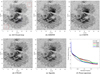 |
Fig. 3 One source image in the first testing set and its corresponding image restored by all methods. Panel a is an AO closed-loop image; panels b–d are the corresponding images restored by EDDNN, CSSTN, and CTSAN; panel e is the corresponding Speckle image (1792 × 1792 pixels). Panel f is the corresponding power spectrum curves of panels a to e. The patches enclosed by color rectangles are detailedly shown in Fig. 4. |
Average PSNR (dB) of the five restored testing sets by EDDNN, CSSTN, and CTSAN.
Lowest, highest, and average granulation contrast and relative improvement on the first testing set.
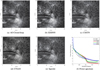 |
Fig. 5 One source image in the second testing set and its corresponding restored images by all methods. Panel a is an AO closed-loop image; panels b to d are the corresponding images restored by EDDNN, CSSTN, and CTSAN; panel e is the corresponding Speckle image (512 × 512 pixels); and panel f is the corresponding power spectrum curves of (a)–(e). |
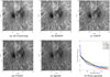 |
Fig. 6 One source image in the third testing set and its corresponding restored images by all methods. Panel a is an AO closed-loop image; panels b–d are the corresponding images restored by EDDNN, CSSTN, and CTSAN; panel e is the corresponding Speckle image (512 × 512 pixels); and panel f is the corresponding power spectrum curves of (a)–(e). |
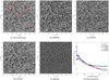 |
Fig. 7 One source image in the fourth testing set and its corresponding restored images by all methods. Panel a is an AO closed-loop image; panels b–d are the corresponding images restored by EDDNN, CSSTN, and CTSAN; panel e is the corresponding Speckle image (1976 × 1976 pixels). Panel f is the corresponding power spectrum curves of panels a–e. The patches enclosed by color rectangles are detailedly shown in Fig. 8. |
Lowest, highest, and average contrast and relative improvement of granulation region on the fourth testing set.
Lowest, highest, and average contrast and relative improvement of granulation subregion on the fifth testing set.
4.2 Ablation study
To better understand and verify each module’s effectiveness in CSTAN, including cascaded two-stage architecture, PWC-Net, TSP, TSA, and HEM, we perform further analysis by a series of ablation studies in Table 8. We first train these ablation models on the first TiO training dataset with 200 epochs. The evaluation results on the first TiO testing set are reflected on both PSNRSingle and SSIMsįngle of Table 8. The average PSNR value among the whole first testing 1000 images of CTSAN (the last line of Table 8) are 0.83 dB, 0.43 dB, 0.32 dB, and 0.05 dB higher than ablation models without cascaded two-stage architecture (second line of Table 8), without TSP (fourth line of Table 8), without TSA (fifth line of Table 8), without HEM (sixth line of Table 8), respectively. The effectiveness of PWC-Net is verified by comparing the third and fourth rows in Table 8, which shows the average PSNR among the whole first testing set of a model with PWC-Net is 0.13 dB higher than the ablation model without PWC-Net module. The SSIMsįngle results also reflect a similar trend to PSNRsįngle, highlighting these modules’ effectiveness in improving network performance.
We also show the ablation model’s results trained on the dual-band training dataset, which has a similar trend to single-band evaluation results in verifying each module’s effectiveness, as the PSNRdual and SSIMdual results shown in Table 8. The dual-band model’s PSNR iteration curves of the PWC-Net and TSP ablation module and CTSAN on the validation set are shown in Fig. 11, which verifies their effectiveness from another perspective. It can be seen that the PSNR iteration curve of the ablation model without PWC-Net has a large variance and fluctuation, while the model with PWC-Net tends to be more stable and smooth, as shown in Figs. 11a,b. It is also evident that the PSNR iteration curve of the model with TSP converges at a higher PSNR value on the validation set than the ablation model without TSP, as shown in Figs. 11b,c.
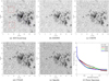 |
Fig. 9 One source image in the fifth testing set and its corresponding restored images by all methods. Panel a is an AO closed-loop image; panels b–d are the corresponding images restored by EDDNN, CSSTN, and CTSAN; panel e is the corresponding Speckle image (1408 × 1408 pixels); and panel f is the corresponding power spectrum curves of (a)–(e). The patches enclosed by color rectangles are detailedly shown in Fig. 10. |
5 Discussion and conclusion
This research proposed a cascaded temporal and spatial network named CTSAN for real solar AO closed-loop image postprocessing. Four modules inside CTSAN, including PWC-Net, TSA, TSP, and HEM, were included for inter-frame explicit alignment, feature fusion, sharp feature extraction, and hard sample mining. We compared the performance of CTSAN with EDDNN and CSSTN in our five real AO testing sets both subjectively and objectively. The results show CTSAN has better precision and generalization abilities and is more robust in restoring the short-exposure AO frames with the lowest granulation subregion contrast. Finally, ablation studies were evaluated on our first testing set to verify the modules’ effectiveness preliminarily.
CTSAN and the other two supervised networks were evaluated on five real testing sets using PSNR, power spectrum, granulation contrast, and relative improvement as quantitative metrics. From the power spectrum curve, CTSAN’s curve is closer to Speckle’s curve than EDDNN and CSSTN, especially in the mid-to high-frequency range, indicating CTSAN restored results have the closest appearance with Speckle in edges, boundaries, and texture details. The qualitative testing results validate CTSAN has better feasibility and effectiveness for improving solar AO closed-loop image quality and restoring details. In particular, our network has a better performance than CSSTN and EDDNN on the lowest granulation contrast frames in three TiO testing sets shown in Tables 6 and 7, indicating that our cascaded network may be able to maintain stable performance in astronomical observation conditions not seen in training. We also employed the trained CTSAN model to directly restore the image patches with 256 × 256 pixels of the first testing set. The qualitative and quantitative evaluation results are similar to Fig. 4d, indicating our method is robust in spatially variant and spatially invariant situations.
When restoring multi-frame solar AO sequences, taking advantage of information transferring from adjacent frames and previous stages is essential. The cascaded architecture has a different information-transferring method than EDDNN and CSSTN. CTSAN only depends on the input of the current five consecutive frames, as shown in Fig. 1c, and does not rely on previous restored images. This implementation prevents previous side effects on current and later image reconstruction. Conversely, CSSTN uses the previously restored image to reach the purpose of information transferring. We found that the results of CSSTN have a smaller difference in appearance compared to CTSAN on the normal source AO image, but have a noticeably greater difference to CTSAN on the lowest granulation contrast images, as shown in Fig. 9c. These phenomena indicate that the stability of CTSAN is better than CSSTN. As a simple and real-time network with an encoder-decoder architecture, EDDNN employs seven frames of the burst to restore one solar AO image. However, its performance needs further improvement than CSSTN and CTSAN in all five real testing sets. It indicates that more than a single encoder-decoder architecture is needed for an end-to-end restoring network.
CTSAN has more obvious superior performance than EDDNN and CSSTN in restoring granulation among all typical sun areas. PWC-Net may contribute to correcting well in low-order biases, leading to better results in the granulation area. Generally speaking, the AO system can better restore the middle region of a FoV (Kong et al. 2017; Scharwaechter et al. 2019). Therefore, granulation regions are farther from the center and contain more lower-order biases in our three 705 nm photosphere testing sets. These better results than CSSTN also indicate that our explicit alignment is better than implicit alignment in CSSTN. We validate the effectiveness of PWC-Net in inter-frame alignment by ablation experiments, as shown in Table 8 and Fig. 11. Our inter-frame alignment in PWC-Net uses pixel-level explicit alignment, which is a more precise alignment (Sun et al. 2018; Gu et al. 2019). In the future, we would consider finding other registration methods that may yield better aligned features in geometric variation regions, such as deformable alignment (Chan et al. 2021).
However, our proposed network still has some limitations. One practical limitation of our CTSAN is that we spend more time on both training and inference. Although our CTSAN has fewer memory allocation requirements than CSSTN in inferencing TiO high-resolution images, our CTSAN spends about 10 s restoring a 1792 × 1792 pixel image with a single RTX3090 in our server. Some efforts are still needed to apply this method in real-time astronomical observation. Employing knowledge distillation to get a compact model with less inference time and model parameters is a possible and practical solution (Suin et al. 2021; Wang & Yoon 2021). Applied scientists can also train with the newest Pytorch 2.0 + version, which has a far higher training speed than the version we used, Pytorch 1.13.0, or can choose a parallel multi-GPU training strategy to accelerate training. Moreover, model performance may be further improved by designing cascaded three or more stage networks while keeping the number of trainable parameters constant.
In addition to the common data enhancement methods for small training samples used in this article, one of the classical methods in astronomical image restoration is using synthetic data to expand training sets, thus preventing overfitting in small training samples (Löfdahl & Hillberg 2022). We also find that the 705 nm training set contributes to preventing overfit-ting when training the 656 nm restoration model with a small 656 nm training set. Other restrictions of our algorithm applied in restoring solar AO image post-processing are the limited inter-pretability. Other sophisticated and more interpretable processes, such as self-attention and diffusion probabilistic models, may be worth exploring further (Deng et al. 2021; Song et al. 2022). Meanwhile, compared with non-deep learning methods of restoring solar AO images (Wang et al. 2022), a systematic theory of deep learning is urgently needed to support its wide application in actual astronomy imaging and observation scenario requiring high reliability and interpretability.
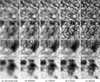 |
Fig. 10 Four subregion images corresponding to the rectangular patches in Fig. 9a (256 × 256 pixels). |
Ablation studies using single-band and dual-band trained models to restore the whole first testing set to verify the effectiveness of cascaded two-stage manner, PWC-net, TSP, TSA, and HEM module of our proposed network.
 |
Fig. 11 Dual-band PSNR iteration curve of the PWC-Net and TSP ablation model evaluated on the validation set. |
Acknowledgements
This work is partly supported by the National Natural Science Foundation of China (NSFC) numbers 11727805, 11703029, and 11733005 and the Municipal Government of Quzhou, 2022D025.
References
- Armstrong, J. A., & Fletcher, L. 2021, MNRAS, 501, 2647 [NASA ADS] [CrossRef] [Google Scholar]
- Asensio Ramos, A., & Olspert, N. 2021, A&A, 646, A100 [NASA ADS] [CrossRef] [EDP Sciences] [Google Scholar]
- Asensio Ramos, A., de la Cruz Rodríguez, J., & Yabar, A. P. 2018, A&A, 620, A73 [NASA ADS] [CrossRef] [EDP Sciences] [Google Scholar]
- Bao, H., Rao, C., Tian, Y., et al. 2018, Opto-Electronic Eng., 45, 170730 [Google Scholar]
- Baranec, C., Riddle, R., Law, N. M., et al. 2014, ApJ, 790, L8 [NASA ADS] [CrossRef] [Google Scholar]
- Baso, C. D., de la Cruz Rodriguez, J., & Danilovic, S. 2019, A&A, 629, A99 [NASA ADS] [CrossRef] [EDP Sciences] [Google Scholar]
- Blanc, A., Fusco, T., Hartung, M., Mugnier, L., & Rousset, G. 2003, A&A, 399, 373 [NASA ADS] [CrossRef] [EDP Sciences] [Google Scholar]
- Butler, D. J., Wulff, J., Stanley, G. B., & Black, M. J. 2012, in European Conference on Computer Vision (Berlin: Springer), 611 [Google Scholar]
- Carbillet, M., Ferrari, A., Aime, C., Campbell, H., & Greenaway, A. 2006, Eur. Astron. Soc. Pub. Ser., 22, 165 [Google Scholar]
- Chan, K. C., Wang, X., Yu, K., Dong, C., & Loy, C. C. 2021, in Proceedings of the AAAI conference on artificial intelligence, 35, 2, 973 [CrossRef] [Google Scholar]
- Cho, S., Wang, J., & Lee, S. 2012, ACM Trans. Graphics, 31, 1 [CrossRef] [Google Scholar]
- Codona, J. L., & Kenworthy, M. 2013, ApJ, 767, 100 [NASA ADS] [CrossRef] [Google Scholar]
- Deng, J., Song, W., Liu, D., et al. 2021, ApJ, 923, 76 [CrossRef] [Google Scholar]
- Ehret, T., Davy, A., Morel, J.-M., Facciolo, G., & Arias, P. 2019, in Proceedings of the IEEE/CVF Conference on Computer Vision and Pattern Recognition, 11369 [Google Scholar]
- Fei, X., Zhao, J., Zhao, H., Yun, D., & Zhang, Y. 2017, Biomedical Opt. Express, 8, 5675 [CrossRef] [Google Scholar]
- Fortun, D., Bouthemy, P., & Kervrann, C. 2015, Computer Vision and Image Understanding, 134, 1 [CrossRef] [Google Scholar]
- Gu, D., Wen, Z., Cui, W., et al. 2019, in International Conference on Multimedia and Expo, IEEE, 1768 [Google Scholar]
- Guo, Y., Zhong, L., Min, L., et al. 2022, Opto-Electronic Adv., 5, 200082 [CrossRef] [Google Scholar]
- Haffert, S. Y., Males, J. R., Close, L. M., et al. 2022, SPIE, 12185, 1071 [Google Scholar]
- He, D., Song, Y., Jin, D., et al. 2021, in Proceedings of the twenty-ninth international conference on international joint conferences on artificial intelligence, 3515 [Google Scholar]
- He, K., Chen, X., Xie, S., et al. 2022, in Proceedings of the IEEE/CVF Conference on Computer Vision and Pattern Recognition, 16000 [Google Scholar]
- Hinnen, K., Verhaegen, M., & Doelman, N. 2008, IEEE Transac. Control Syst. Technol., 16, 381 [Google Scholar]
- Hore, A., & Ziou, D. 2010, in 20th international conference on pattern recognition, IEEE, 2366 [Google Scholar]
- Hyun Kim, T., & Mu Lee, K. 2015, in Proceedings of the IEEE Conference on Computer Vision and Pattern Recognition, 5426 [Google Scholar]
- Jia, P., Huang, Y., Cai, B., & Cai, D. 2019, ApJ, 881, L30 [NASA ADS] [CrossRef] [Google Scholar]
- Jiang, W. 2018, Opto-Electronic Eng., 45, 170489 [Google Scholar]
- Jiang, H., Zhou, Y., Lin, Y., et al. 2022, Med. Image Anal., 84, 102691 [Google Scholar]
- Kaufman, A., & Fattal, R. 2020, in Proceedings of the IEEE/CVF conference on computer vision and pattern recognition, 5811 [Google Scholar]
- Keller, C., & Von Der Luehe, O. 1992, A&A, 261, 321 [Google Scholar]
- Kong, L., Zhang, L., Zhu, L., et al. 2016, Chinese Opt. Lett., 14, 100102 [CrossRef] [Google Scholar]
- Kong, L., Zhu, L., Zhang, L., Bao, H., & Rao, C. 2017, IEEE Photon. J., 9, 1 [Google Scholar]
- Lai, H.-Y., Tsai, Y.-H., & Chiu, W.-C. 2019, in Proceedings of the IEEE/CVF Conference on Computer Vision and Pattern Recognition, 1890 [Google Scholar]
- Liang, J., Williams, D. R., & Miller, D. T. 1997, JOSA A, 14, 2884 [CrossRef] [PubMed] [Google Scholar]
- Lim, B., Son, S., Kim, H., Nah, S., & Mu Lee, K. 2017, in Proceedings of the IEEE conference on computer vision and pattern recognition workshops, 136 [Google Scholar]
- Löfdahl, M. G., & Hillberg, T. 2022, A&A, 668, A129 [NASA ADS] [CrossRef] [EDP Sciences] [Google Scholar]
- Lukin, V., Antoshkin, L., Bolbasova, L., et al. 2020, Atmos. Oceanic Opt., 33, 85 [CrossRef] [Google Scholar]
- Maurer, D., & Bruhn, A. 2018, British Mach. Vision Conf., 2018, 86 [Google Scholar]
- Meister, S., Hur, J., & Roth, S. 2018, in Proceedings of the Thirty-Second AAAI Conference on Artificial Intelligence, 7251 [Google Scholar]
- Menze, M., & Geiger, A. 2015, in Proceedings of the IEEE conference on computer vision and pattern recognition, 3061 [Google Scholar]
- Otte, M., & Nagel, H.-H. 1994, in European conference on computer vision, Springer, 49 [Google Scholar]
- Pan, J., Bai, H., & Tang, J. 2020, in Proceedings of the IEEE/CVF Conference on Computer Vision and Pattern Recognition, 3043 [Google Scholar]
- Rao, C., & Jiang, W. 2002, SPIE, 4926, 20 [NASA ADS] [Google Scholar]
- Rao, C., Jiang, W., Fang, C., et al. 2003, Chinese J. Astron. Astrophys., 3, 576 [CrossRef] [Google Scholar]
- Rao, C., Zhu, L., Rao, X., et al. 2015, Chinese Opt. Lett., 13, 120101 [NASA ADS] [CrossRef] [Google Scholar]
- Rao, C., Zhu, L., Rao, X., et al. 2016a, ApJ, 833, 210 [NASA ADS] [CrossRef] [Google Scholar]
- Rao, C., Zhu, L., Rao, X., et al. 2016b, Res. Astron. Astrophys., 16, 003 [CrossRef] [Google Scholar]
- Rao, C., Lei, Z., Lanqiang, Z., et al. 2018, Opto-Electronic Eng., 45, 170733 [Google Scholar]
- Rao, C., Gu, N., Rao, X., et al. 2020, Sci. China Phys. Mech. Astron., 63, 109631 [CrossRef] [Google Scholar]
- Ratnasingam, S. 2019, in Proceedings of the IEEE/CVF International Conference on Computer Vision Workshops [Google Scholar]
- Restaino, S. R. 1992, Appl. Opt., 31, 7442 [NASA ADS] [CrossRef] [Google Scholar]
- Rimmele, T. R., & Marino, J. 2011, Liv. Rev. Sol. Phys., 8, 1 [NASA ADS] [Google Scholar]
- Rousset, G., Fontanella, J., Kern, P., Gigan, P., & Rigaut, F. 1990, A&A, 230, L29 [Google Scholar]
- Salter, P. S., & Booth, M. J. 2019, Light Sci. Applications, 8, 1 [NASA ADS] [CrossRef] [Google Scholar]
- Scharwaechter, J., Andersen, M., Sivo, G., & Blakeslee, J. 2019, AO4ELT6 Proc [Google Scholar]
- Song, W., Ma, W., Ma, Y., Zhao, X., & Lin, G. 2022, ApJS, 263, 25 [NASA ADS] [CrossRef] [Google Scholar]
- Stachnik, R., Nisenson, P., Ehn, D., Hudgin, R., & Schirf, V. 1977, Nature, 266, 149 [NASA ADS] [CrossRef] [Google Scholar]
- Suin, M., Purohit, K., & Rajagopalan, A. N. 2021, IEEE J. Selected Topics in Signal Process., 15, 162 [NASA ADS] [CrossRef] [Google Scholar]
- Sun, D., Yang, X., Liu, M.-Y., & Kautz, J. 2018, in Proceedings of the IEEE conference on computer vision and pattern recognition, 8934 [Google Scholar]
- Tao, X., Gao, H., Shen, X., Wang, J., & Jia, J. 2018, in Proceedings of the IEEE Conference on Computer Vision and Pattern Recognition, 8174 [Google Scholar]
- Tian, Y., Rao, C., & Wei, K. 2008, SPIE, 7015, 655 [Google Scholar]
- Tian, C., Fei, L., Zheng, W., et al. 2020, Neural Netw., 131, 251 [Google Scholar]
- van Noort, M., Rouppe van der Voort, L., & Löfdahl, M. 2006, ASP Conf. Ser., 354, 55 [NASA ADS] [Google Scholar]
- Vaswani, A., Shazeer, N., Parmar, N., et al. 2017, in Advances in neural information processing systems, 5998 [Google Scholar]
- Voulodimos, A., Doulamis, N., Doulamis, A., & Protopapadakis, E. 2018, Comput. Intell. Neurosci., 2018, 1 [Google Scholar]
- Wang, L., & Yoon, K.-J. 2021, IEEE Transactions on Pattern Analysis and Machine Intelligence 44, 6, 3048 [Google Scholar]
- Wang, X., Yu, K., Dong, C., & Loy, C. C. 2018, in Proceedings of the IEEE conference on computer vision and pattern recognition, 606 [Google Scholar]
- Wang, X., Chan, K. C., Yu, K., Dong, C., & Change Loy, C. 2019, in Proceedings of the IEEE/CVF Conference on Computer Vision and Pattern Recognition Workshops, 0 [Google Scholar]
- Wang, S., Chen, Q., He, C., et al. 2021, A&A, 652, A50 [NASA ADS] [CrossRef] [EDP Sciences] [Google Scholar]
- Wang, S., Rong, H., He, C., Zhong, L., & Rao, C. 2022, ASP Conf. Ser., 134, 064502 [Google Scholar]
- Wang, S., He, C., Rong, H., et al. 2023, Opto-Electronic Eng., 50, 220207 [Google Scholar]
- Wedemeyer-Böhm, S., & van der Voort, L. R. 2009, A&A, 503, 225 [NASA ADS] [CrossRef] [EDP Sciences] [Google Scholar]
- Welsh, B. M., & Roggemann, M. C. 1995, Appl. Opt., 34, 2111 [NASA ADS] [CrossRef] [Google Scholar]
- Weyrauch, T., Vorontsov, M. A., Gowens, J., & Bifano, T. G. 2002, SPIE, 4489, 177 [NASA ADS] [Google Scholar]
- Xiang, X., Wei, H., & Pan, J. 2020, IEEE Transac. Image Process., 29, 8976 [CrossRef] [Google Scholar]
- Xu, R., Li, X., Zhou, B., & Loy, C. C. 2019, in Proceedings of the IEEE/CVF Conference on Computer Vision and Pattern Recognition, 3723 [Google Scholar]
- Ye, S., He, Q., & Wang, X. 2021, in 2021, Radar Conference, IEEE, 1 [Google Scholar]
- Zamir, S. W., Arora, A., Khan, S., et al. 2021, in Proceedings of the IEEE/CVF Conference on Computer Vision and Pattern Recognition, 14821 [Google Scholar]
- Zhang, Y., Ye, T., Xi, H., Juhas, M., & Li, J. 2021, Front. Microbiol., 12, 739684 [CrossRef] [Google Scholar]
- Zhang, K., Ren, W., Luo, W., et al. 2022, Int. J. Comput. Vision, 1 [Google Scholar]
- Zhong, L., Tian, Y., & Rao, C. 2014, Opt. Exp., 22, 29249 [CrossRef] [Google Scholar]
- Zhong, L., Zhang, L., Shi, Z., et al. 2020, A&A, 637, A99 [NASA ADS] [CrossRef] [EDP Sciences] [Google Scholar]
- Zou, X., Yang, L., Liu, D., & Lee, Y. J. 2021, in Proceedings of the IEEE/CVF Conference on Computer Vision and Pattern Recognition, 16448 [Google Scholar]
All Tables
Architecture of spatial attention part in TSA Module with upsampling implemented by bilinear interpolation.
Lowest, highest, and average granulation contrast and relative improvement on the first testing set.
Lowest, highest, and average contrast and relative improvement of granulation region on the fourth testing set.
Lowest, highest, and average contrast and relative improvement of granulation subregion on the fifth testing set.
Ablation studies using single-band and dual-band trained models to restore the whole first testing set to verify the effectiveness of cascaded two-stage manner, PWC-net, TSP, TSA, and HEM module of our proposed network.
All Figures
|
Fig. 1 Overview of proposed CTSAN architecture. Panel a shows the network detail of the TSAN unit. Panel b is the input and output of a single TSAN unit. Panel c shows the forward propagation process of CTSAN. The same trained TSAN parameter is used four times to construct the cascaded two-stage architecture. |
| In the text | |
|
Fig. 2 Architecture of TSA module for feature fusion. The output feature of temporal attention is modulated by the fusion convolution block before feeding into the spatial attention module. |
| In the text | |
|
Fig. 3 One source image in the first testing set and its corresponding image restored by all methods. Panel a is an AO closed-loop image; panels b–d are the corresponding images restored by EDDNN, CSSTN, and CTSAN; panel e is the corresponding Speckle image (1792 × 1792 pixels). Panel f is the corresponding power spectrum curves of panels a to e. The patches enclosed by color rectangles are detailedly shown in Fig. 4. |
| In the text | |
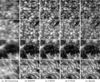 |
Fig. 4 Four subregion images corresponding to the patches in Fig. 3a (256 × 256 pixels). |
| In the text | |
|
Fig. 5 One source image in the second testing set and its corresponding restored images by all methods. Panel a is an AO closed-loop image; panels b to d are the corresponding images restored by EDDNN, CSSTN, and CTSAN; panel e is the corresponding Speckle image (512 × 512 pixels); and panel f is the corresponding power spectrum curves of (a)–(e). |
| In the text | |
|
Fig. 6 One source image in the third testing set and its corresponding restored images by all methods. Panel a is an AO closed-loop image; panels b–d are the corresponding images restored by EDDNN, CSSTN, and CTSAN; panel e is the corresponding Speckle image (512 × 512 pixels); and panel f is the corresponding power spectrum curves of (a)–(e). |
| In the text | |
|
Fig. 7 One source image in the fourth testing set and its corresponding restored images by all methods. Panel a is an AO closed-loop image; panels b–d are the corresponding images restored by EDDNN, CSSTN, and CTSAN; panel e is the corresponding Speckle image (1976 × 1976 pixels). Panel f is the corresponding power spectrum curves of panels a–e. The patches enclosed by color rectangles are detailedly shown in Fig. 8. |
| In the text | |
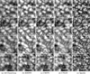 |
Fig. 8 Four subregion images corresponding to the rectangular patches in Fig. 7a (256 × 256 pixels). |
| In the text | |
|
Fig. 9 One source image in the fifth testing set and its corresponding restored images by all methods. Panel a is an AO closed-loop image; panels b–d are the corresponding images restored by EDDNN, CSSTN, and CTSAN; panel e is the corresponding Speckle image (1408 × 1408 pixels); and panel f is the corresponding power spectrum curves of (a)–(e). The patches enclosed by color rectangles are detailedly shown in Fig. 10. |
| In the text | |
|
Fig. 10 Four subregion images corresponding to the rectangular patches in Fig. 9a (256 × 256 pixels). |
| In the text | |
|
Fig. 11 Dual-band PSNR iteration curve of the PWC-Net and TSP ablation model evaluated on the validation set. |
| In the text | |
Current usage metrics show cumulative count of Article Views (full-text article views including HTML views, PDF and ePub downloads, according to the available data) and Abstracts Views on Vision4Press platform.
Data correspond to usage on the plateform after 2015. The current usage metrics is available 48-96 hours after online publication and is updated daily on week days.
Initial download of the metrics may take a while.