| Issue |
A&A
Volume 652, August 2021
|
|
|---|---|---|
| Article Number | A129 | |
| Number of page(s) | 10 | |
| Section | Galactic structure, stellar clusters and populations | |
| DOI | https://doi.org/10.1051/0004-6361/202140347 | |
| Published online | 23 August 2021 | |
An intriguing globular cluster in the Galactic bulge from the VVV survey⋆
1
Departamento de Ciencias Físicas, Facultad de Ciencias Exactas, Universidad Andres Bello, Fernández Concha 700, Las Condes, Santiago, Chile
e-mail: This email address is being protected from spambots. You need JavaScript enabled to view it.
2
Vatican Observatory, Vatican City State 00120, Italy
3
Observatorio Astronómico, Universidad Nacional de Córdoba, Laprida 854, 5000 Córdoba, Argentina
4
Consejo Nacional de Investigaciones Científicas y Técnicas (CONICET), Godoy Cruz 2290, Ciudad Autónoma de Buenos Aires, Argentina
5
Colégio Militar de Porto Alegre, Ministério da Defesa, Av. José Bonifácio 363, Porto Alegre, 90040-130 RS, Brazil
6
Centro de Astronomía (CITEVA), Universidad de Antofagasta, Av. Angamos 601, Antofagasta, Chile
7
Millennium Institute of Astrophysics, Nuncio Monseñor Sotero Sanz 100, Of. 104, Providencia, Santiago, Chile
8
Instituto de Alta Investigación, Sede Iquique, Universidad de Tarapacá, Av. Luis Emilio Recabarren 2477, Iquique, Chile
9
Departamento de Física, Universidade Federal de Santa Catarina, Trindade, 88040-900 Florianópolis, SC, Brazil
Received:
14
January
2021
Accepted:
23
June
2021
Abstract
Context. Globular clusters (GCs) are the oldest objects known in the Milky Way, so each discovery of a new GC is astrophysically important. In the inner Galactic bulge regions these objects are difficult to find due to extreme crowding and extinction. However, recent near-IR surveys have discovered a number of new bulge GC candidates that need to be further investigated.
Aims. Our main objective is to use public data from the Gaia mission, the VISTA Variables in the Via Lactea (VVV) survey, the Two Micron All Sky Survey, and the Wide-field Infrared Survey Explorer to measure the physical parameters of Minni 48, a new candidate globular star cluster located in the inner bulge of the Milky Way at l = 359.35 deg, b = 2.79 deg. The specific goals are to measure its main astrophysical parameters, such as size, proper motions, metallicity, reddening and extinction, distance, total luminosity, and age.
Methods. Even though there is a bright foreground star contaminating the field, this cluster appears quite bright in near- and mid-IR images. The size of Minni 48 is derived from the cluster radial density profile, while its reddening and extinction are estimated from optical and near-IR reddening maps. We obtain statistically decontaminated optical and near-IR colour-magnitude diagrams (CMDs) for this cluster. Mean cluster proper motions are measured from Gaia data. The heliocentric cluster distance is determined from both the red clump (RC) and the red giant branch (RGB) tip magnitudes in the near-IR CMD, while the cluster metallicity is estimated from the RGB slope and the fit to theoretical stellar isochrones.
Results. The size of this GC is found to be r = 6′±1′, and the reddening and extinction values are E(J − Ks) = 0.60 ± 0.05 mag, AG = 3.23 ± 0.10 mag, and AKs = 0.45 ± 0.05 mag. The resulting mean cluster proper motions are μα = −3.5 ± 0.5 mas yr−1 and μδ = −6.0 ± 0.5 mas yr−1. We also study the RR Lyrae stars recognized in the field, and we argue that they are not members of this GC. The magnitude of the RC in the near-IR CMD yields an accurate distance modulus estimate of (m − M)0 = 14.61 mag, equivalent to a distance D = 8.4 ± 1.0 kpc. Such a distance is consistent with the optical distance estimate, (m − M)0 = 14.67 mag, D = 8.6 ± 1.0 kpc, as well as with the distance estimated using the tip of the RGB, (m − M)0 = 14.45 mag, D = 7.8 ± 1.0 kpc. We also derive a cluster metallicity of [Fe/H] = − 0.20 ± 0.30 dex. Adopting these values of metallicity and distance, a good fit to the PARSEC stellar isochrones is obtained in all CMDs using Age = 10 ± 2 Gyr. The total absolute magnitude of this GC is estimated to be MKs = −9.04 ± 0.66 mag.
Conclusions. Based on its position, kinematics, metallicity, and age, we conclude that Minni 48 is a genuine GC, similar to other well-known metal-rich bulge GCs. It is located at a projected galactocentric angular distance of 2.9 deg, equivalent to 0.4 kpc, situating this cluster as one of the closest GCs to the Galactic centre currently known.
Key words: stars: variables: RR Lyrae / Galaxy: bulge / globular clusters: general
Based on observations taken within the ESO VISTA public survey VVV, Programme ID 198.B-2004.
© ESO 2021
1. Introduction
The inner Galactic bulge globular clusters (GCs) are particularly difficult to find and to characterize at optical wavelengths due to heavy interstellar extinction and severe stellar crowding. Recent near-IR surveys – the Two Micron All Sky Survey (2MASS; Skrutskie et al. 2006) and the VISTA Variables in the Via Lactea (VVV) survey (Minniti et al. 2010) – and mid-IR surveys – the Spitzer Galactic Legacy Infrared Mid-Plane Survey Extraordinaire (GLIMPSE; Benjamin et al. 2003) and the Wide-field Infrared Survey Explorer (WISE; Wright et al. 2010) – have meant a real revolution for the study of GCs in the Milky Way (MW) bulge.
On one hand, the deep near- and mid-IR images led to the discovery of dozens of new GC candidates in the bulge that had hitherto remained hidden due to the high crowding and severe differential reddening in the inner regions of the Galaxy. For example, Camargo et al. (2015, 2016) developed a star cluster survey using WISE images, which allowed for the discovery of eight new bulge GCs (Camargo 2018; Camargo & Minniti 2019).
On the other hand, the near- and mid-IR photometry and the multi-epoch observations of variable stars have permitted the accurate measurement of the physical parameters (sizes, reddenings, distances, ages, luminosities, etc.) for several of the known GCs that have been studied so far (e.g., Longmore et al. 2011; Minniti et al. 2011, 2017a,b; Moni-Bidin et al. 2011; Ortolani et al. 2012; Alonso-García et al. 2015; Borissova et al. 2014; Piatti 2018; Ryu & Lee 2018; Palma et al. 2019). These studies have contributed to a deeper understanding of the formation and evolution of the MW GC system.
At the distance of the bulge, the GLIMPSE and WISE mid-IR surveys are sensitive to the clusters’ bright red giants (RGs). The 2MASS catalogue allows the cluster upper red giant branch (RGB), used to measure the RGB tip and the RGB slope, to be defined. The VVV photometry samples deeper into the RGB, making it possible to measure the horizontal branch (HB) shape and the red clump (RC) magnitude. These near- and mid-IR surveys, in combination with the optical photometry and proper motions (PMs) from the Gaia mission (Gaia Collaboration 2018a), can be used to measure the cluster physical parameters, including position, PMs, size, metallicity, luminosity, reddening, and extinction, as well as age using isochrones fitted to the observed cluster sequence.
In this paper we concentrate on a fairly rare object, the candidate GC Minni 48. Using the VVV survey, this candidate GC was discovered as a concentration of RR Lyrae and RGs, suggesting a metal-poor GC (Minniti et al. 2018). However, a later examination of the mid-IR GLIMPSE and WISE images showed a cluster that appears quite bright at these wavelengths, suggesting a metal-rich GC. Interestingly, the Gaia Early Data Release 3 (EDR3) colour-magnitude diagram (CMD) shows that the upper giant branch in the cluster region is well split into a bluer and a redder RGB, as shown in Fig. 1 (the Gaia DR2 CMD shows a similar upper RGB split).
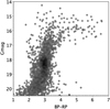 |
Fig. 1. Gaia EDR3 optical CMD (G vs. BP–RP) for a r < 3′ region centred in the GC. This CMD shows that the upper RGB in this area is clearly split into a bluer and a redder component. |
This cluster is located along the Galactic minor axis (l = −0.65 deg) at a low latitude (b = +2.79 deg). This is one of the closest clusters to the Galactic centre, with a projected galactocentric angular distance of r = 2.9 deg. A major complication for its study is the high field stellar density wherein it is projected, which is even higher than that of Baade’s window at b = −4 deg, a window of low extinction also located along the minor axis but on the other side of the Galactic plane, where the classical GCs NGC 6522 and NGC 6528 are found.
Another obstacle for the study of this object is the presence of a very bright foreground stellar source (IRAS 17302-2800, also known as 2MASS 17331634-2800145), projected near its centre. With magnitudes Ks = 3.33 and G = 10.57 and colour indexes (J − Ks) = 1.81 and (BP − RP) = 5.60, this star is badly saturated in optical and IR images, affecting the photometry of the surrounding region. In fact, we argue that Minni 48 is an ordinary GC that had previously been missed due precisely to the presence of this bright source. On the other hand, it should be noted that even in the presence of a bright foreground star, it is possible to recover the underlying cluster, as shown for example by the discovery of one of the first Gaia clusters (Koposov et al. 2017).
2. The optical and IR datasets
Given that the stellar density is so high in the cluster region, we must make sure of the measured location of the RGB and RC, which determine important cluster parameters such as reddening, distance and metallicity. For this reason, we use all available optical and near-IR data. Fortunately, we are able to come to a consistent solution across all wavelengths.
The examination of the GC appearance in the sky reveals a clear excess of stars with respect to the background. This excess is more conspicuous at the RGB tip in the 2MASS CMDs and at the RC regions of the VVV and Dark Energy Camera Plane Survey (DECaPS) CMDs, although at the shorter wavelengths it is more difficult to appreciate because it is eclipsed by the bright star (Fig. 2). Such excess is prominent when we restrict the comparison to stars kinematically selected using Gaia EDR3 PMs. A brief description of the available datasets along with the relevant references is presented below.
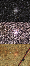 |
Fig. 2. Zoomed-in views of a 9′×7′ region centred on Minni 48 obtained with VVV (top panel), 2MASS (middle panel), and DECaPS (bottom panel) This figure is oriented along equatorial coordinates, with east to the left and north to the top (see also Fig. 3). The white arrows point to the RR Lyrae stars and the yellow arrow to the Type 2 Cepheid. The saturated star near the centre is the bright source IRAS 17302-2800, with Ks = 3.33 and (J − Ks) = 1.81 mag. |
2.1. 2MASS photometry for bright stars
The 2MASS is an all sky survey in the JHKs near-IR bands (Skrutskie et al. 2006; Cutri et al. 2003). We retrieved the 2MASS data from the VizieR Online Data Catalogue. Since the brightest stars in Minni 48 (Ks < 11 mag) appear to be saturated in the VVV near-IR images (Saito et al. 2012), we use 2MASS data in order to build the complete CMD. The first selection applied here culls stars with large photometric errors: σJ > 0.3 mag, and σKs > 0.3 mag. The 2MASS photometry is also linearly related to the VVV photometry (for a detailed description see Mauro et al. 2013; Soto et al. 2013 and González-Fernández et al. 2018).
2.2. Deep VVV survey observations
The VVV survey and its extension, the VVVX survey, are large ESO public near-IR surveys of the southern MW plane (Minniti et al. 2010, 2018). Data reduction was carried out at the Cambridge Astronomical Survey Unit (CASU; Irwin et al. 2004; Lewis et al. 2010). The point spread function (PSF) photometry was extracted using the pipeline described in Alonso-García et al. (2018). The resulting catalogues are in the VISTA photometric system, which is different but related to the 2MASS photometric system (Mauro et al. 2013; Soto et al. 2013; González-Fernández et al. 2018).
Minni 48 is located in the VVV tile b361, a very reddened and crowded bulge field. No photometric or colour cuts were applied to its VVV PSF photometry. As in our analysis the catalogues from 2MASS and VVV were treated independently, we kept the VVV catalogue for Minni 48 in its original VISTA photometric system. We also note that the present VVV calibration should be trusted to ΔJKs < 0.05 mag because some field zero-point variations have been reported in the VVV photometry (Hajdu et al. 2020), although in the present case such a difference could also be partly due to the influence of the bright foreground source IRAS 17302-2800, which affects the background in the VVV images.
2.3. GLIMPSE and WISE mid-IR photometry
The GLIMPSE is a survey of the Galactic plane in four mid-IR bands centred at 3.6, 4.5, 5.8 and 8.0 microns (Benjamin et al. 2003; Churchwell et al. 2009). The WISE is an all-sky survey (Wright et al. 2010) that uses four mid-IR bands, W1, W2, W3, and W4, centred at 3.3, 4.7, 12, and 24 microns, respectively, with lower spatial resolution (6″ − 10″). Visual inspection of the WISE images (Fig. 3) reveals that Minni 48 is prominent and bright in the mid-IR, exhibiting a compact core of bright stars. This is confirmed also by the GLIMPSE image data that has a higher resolution (1″ − 2″).
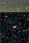 |
Fig. 3. Near and mid-IR views of the new GC. Top: wide field JHKs mosaic covering the VVV tiles b359 to b361, showing the positions of Minni 48 compared with those of the two well-known GCs: HP 1 and Terzan 2. This field, covering approximately 1.5° ×4°, is oriented along Galactic coordinates, with longitudes increasing to the left and latitudes to the top. Bottom: zoomed-in view of a 20′×20′ region centred on Minni 48 obtained with WISE in the mid-IR (3.6–8 microns). There is a clear concentration of bright IR stars in the cluster core. The white box shows the location of the zoomed-in images portrayed in Fig. 2. |
We retrieved from the VizieR Online Data Catalogue the WISE data for the four mid-IR bands W1, W2, W3, and W4. Figure 4 shows the spatial distribution of WISE sources in Galactic coordinates and the corresponding WISE mid-IR CMD. This WISE CMD exhibits the presence of very red stars, generally indicative of evolved metal-rich stars. We find that there is a clear concentration of many RGs in the cluster core (within 3′ of the cluster centre). There are ten very red stars with W1 − W2 > 0.1 mag in a 10′ field centred on the cluster, with five out of these red stars being within 3′ of the centre. The brightest star with W1 = 2.1 mag is the foreground source IRAS 17302-2800.
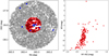 |
Fig. 4. Map of WISE sources (left panel) and a WISE mid-IR CMD (right panel). There is a clear concentration of many RGs in the cluster core. The brightest IR stars are indicated with blue circles. The brightest star, with W1 = 2.1, W1 − W2 = 0 mag, is the foreground source IRAS 17302-2800, which is located close to the cluster centre. For comparison, the region where the Gaia-EDR3 CMD of Fig. 1 is made (r < 3′) is the inner red region shown in this map. |
2.4. Gaia optical photometry and proper motions
We used Gaia DR2 data (Gaia Collaboration 2018a) and EDR3 data (Gaia Collaboration 2021) retrieved from the VizieR Online Data Catalogue. The first selection excludes all nearby foreground stars with plx > 0.5 mas (i.e. D < 3 kpc; Gaia Collaboration 2018b; Bailer-Jones et al. 2018). No photometric colour or magnitude cuts were applied to the Gaia data.
2.5. DECaPS optical photometry
The DECaPS is an optical survey of the Southern Galactic plane and bulge fields with −5 < b < 5 deg (Schlafly et al. 2017). We use the DECaPS fluxes in griYz converted to magnitudes, retrieved from their web page (Schlafly et al. 2017). This optical PSF photometry is complementary, because it provides different colours, and it is deeper than the Gaia photometry in this field (rlim ∼ 24 mag vs. Glim ∼ 21 mag, respectively).
3. Globular cluster physical parameters
There are some major problems for the study of this GC candidate. First and foremost, there is the issue of high field stellar density. This is a common problem for the study of GCs in the bulge, but it is enhanced in the inner Galactic field studied here. For example, using the deep VVV photometry, we count that there are 66% more RC giants per square degree in this field than at Baade’s window, where the well-known metal-rich GCs NGC 6522 and NGC 6528 are located. This high field contamination (both foreground and background) affects the measurement of the cluster size and total luminosity and is reflected in the large errors that we estimate for these two parameters.
Other serious problems are the high differential reddening and extinction. The shape of the extinction law is known to vary in the inner bulge (e.g., Majaess et al. 2016; Nataf et al. 2016; Alonso-García et al. 2017). This makes it difficult to determine the GC distance and increases the systematic errors. However, different methods (RC in the optical and near-IR and the RGB tip) can be used in this study to check consistency. The uncertainty in the extinction also affects age determination using isochrones, thus yielding large errors. Fortunately, the availability of multi-wavelength photometry allows us to reach a consistent solution, as discussed below.
3.1. Colour-magnitude diagrams
As mentioned before, the very high field contamination (foreground and background) in the cluster field is a serious problem for the determination of the cluster parameters. Giving the variety of datasets for this cluster (VVV, 2MASS, Gaia, DECaPS), we deemed appropriate to make two independent decontamination experiments. The cluster parameters can then be better determined using the decontaminated CMDs.
Thus, aiming to uncover the intrinsic CMD morphology of Minni 48 from the bulge field stars, we apply a field-star decontamination procedure. The algorithm divides the CMDs of the cluster region and of a comparison field into a 3D grid (a magnitude and two colours) measuring the density of stars with compatible magnitude and colours in the correspondent cells. Then, the algorithm removes the expected number of field stars from each cell of the cluster CMD (Bonatto & Bica 2007; Bica et al. 2008; Camargo et al. 2009, 2016). In this work we apply a version of the algorithm to the Gaia photometry. Additionally, we used a similar procedure developed by Palma et al. (2016). These decontamination procedures differ in the comparison field selection, the first used a ring of large area centred in the cluster coordinates while the second used equal area background fields with similar reddening ∼10′ away from the cluster for this purpose.
Figure 5 shows the Gaia EDR3 optical CMDs (G vs. BP − RP) for the GC region (left panel), a background region covering a similar area on the sky as the cluster region (middle panel), and the statistically decontaminated CMD (right panel), following the procedures of Camargo et al. (2009) and Palma et al. (2016). It is expected that the observed CMD of a GC embedded in the bulge dense field that remained hidden until recently shows some similarity to the near-field CMD. Sometimes it is hard to clearly perceive the differences between these CMDs by eye, but the decontamination algorithm works on a statistical basis and is able to uncover the cluster intrinsic CMD by comparing colours and magnitudes of the two stellar contents.
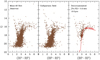 |
Fig. 5. Gaia EDR3 optical CMDs (G vs. BP-RP) for the GC region (left panel), a background region (middle panel), and the statistically decontaminated region following Camargo et al. (2009; right panel). The last CMD clearly shows that only the RGB (more metal rich) survives the decontamination procedure. The Gaia decontaminated CMD is fitted by a PARSEC isochrone with age 10 Gyr and metallicity [Fe/H] = − 0.2 dex. |
The decontaminated CMD on the right panel of Fig. 5 shows that only the RGB (which is more metal rich) survives the decontamination procedure. The bright portion of this optical CMD is easily decontaminated because there is a clear overdensity of luminous cluster stars. The faintest portion, however, is much more difficult to decontaminate because the bright star opaques the fainter ones, and as a result, there is not a clear overdensity with respect to the background. In addition, the accuracy of the photometry may be affected by limitations on the data processing and variations in the local background, in the sense that the Gaia BP and RP fluxes may include contributions of the nearby bright sources. The highest impact occurs for crowded environments, such as the inner regions of GCs and the Galactic bulge. The faint sources are most strongly affected, especially those near bright stars (Arenou et al. 2018; Evans et al. 2018). On the other hand, Gaia obviously still provides a substantial gain in relation to previous large sky surveys.
Figure 6 shows the 2MASS near-IR CMDs (Ks vs. J − Ks) for the GC region (left panel), a background region having a similar area on the sky as the GC region (middle panel), and the statistically decontaminated CMD following Bica et al. (2008) and Camargo et al. (2009; right panel). The decontaminated CMD on the right panel clearly illustrates the metal-rich RGB and the RGB tip located at Ks = 7.75 ± 0.10 mag.
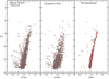 |
Fig. 6. 2MASS near-IR CMDs (Ks vs. J − Ks) for the GC region (left panel), a background region (middle panel), and the statistically decontaminated region following Camargo et al. (2009; right panel). The last CMD clearly shows a tight metal-rich RGB and the RGB tip at Ks = 7.75 ± 0.10 mag. The red line shows a PARSEC isochrone of age 10 Gyr and metallicity [Fe/H] = − 0.2 dex. |
Figure 7 presents the deep VVV near-IR CMDs (Ks vs. J − Ks) for the GC region (left panel), a background region covering a similar area on the sky as the cluster region (middle panel), and the statistically decontaminated CMD following the steps described in detail by Palma et al. (2016; right panel). The decontaminated CMD in the right panel clearly shows the RC of this GC at Ks = 13.45 mag. This feature is important because RC stars are well-known distance indicators (e.g., Girardi 2016) and will be used here to determine the GC distance, adopting KsRC = −1.606 ± 0.009 mag and GRC = 0.383 ± 0.009 mag (Ruiz-Dern et al. 2018).
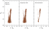 |
Fig. 7. Deep VVV near-IR CMDs (Ks vs. J − Ks) for the GC region (left panel), a background region (middle panel), and the statistically decontaminated region following Palma et al. (2019; right panel). The last CMD clearly shows the GC RC at Ks = 13.45 mag. |
All these CMDs (Figs. 5–7) show that the decontaminated sequence for the cluster is much tighter than that of the background. These datasets have been treated independently, and they all confirm the presence of a real star cluster.
In order to complement the Gaia optical CMDs, Fig. 8 shows the optical CMDs for the GC region from the DECaPS survey (Schlafly et al. 2017). These CMDs are zoomed in the RGB region. They all clearly show the GC RC at r = 18.65 and i = 17.50 mag. We can also appreciate the RGB bump in these diagrams.
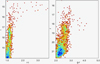 |
Fig. 8. Optical CMDs within 3′ of the GC centre using the DECaPS survey (Schlafly et al. 2017). These diagrams clearly show the GC RC at r = 18.65 and i = 17.50 mag. |
We note that in the presence of differential reddening, if the statistical decontamination procedure leaves abundant field contamination, the mean reddening and metallicity values may be biased. There is another independent way to decontaminate the cluster CMD, and that is using the exquisite astrometry provided by the Gaia mission. In order to do this, we first select all stars within 3′ of the cluster centre with parallaxes smaller than 0.5 mas. This selection eliminates nearby stars belonging to the Galactic disk. After identifying the PM peak due to the GC members in the PM diagram (Fig. 9), we select GC members within 2 mas yr−1, centred on these PMs. The mean cluster PMs measured from Gaia EDR3 are μα = −3.5 ± 0.5 mas yr−1, μδ = −6.0 ± 0.5 mas yr−1. These PM-selected members were then matched with the VVV near-IR photometry and the resulting CMDs are shown in Fig. 10. These CMDs are similar to those obtained using the statistical background decontamination procedure (Figs. 5–7). They almost reach the main sequence turn-off of the cluster, clearly showing a tight RGB and a prominent RC. Figure 11 shows the luminosity functions in the G and Ks-bands, where the RC is clearly seen. This PM decontamination procedure was performed first with Gaia DR2 data and repeated again using Gaia EDR3 data, thus yielding consistent results.
 |
Fig. 9. Gaia-EDR3 vector PM diagrams for the whole 20′ field (left panel) compared with a 5′ field centred on the cluster (right panel) and with an equal area field located 10′ south of the cluster (middle panel). |
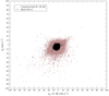 |
Fig. 10. Optical and near-IR CMDs for the GC region after the PM decontamination using Gaia EDR3 data. |
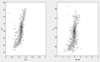 |
Fig. 11. Optical and near-IR CMD luminosity functions (in blue and red, respectively) for the GC region after the PM decontamination using Gaia EDR3 data. |
Figure 12 shows the Gaia EDR3 PM distribution for the Minni 48 central region and for a ring in the comparison field. Minni 48 presents a PM distribution consistent with that of a typical GC located in the Galactic bulge (Camargo 2018; Camargo & Minniti 2019). Figure 12 shows a more compact PM distribution for stars within the cluster area with respect to those in the comparison field, suggesting a cohesive structure. As most bulge GCs, Minni 48 follows the local bulge stellar content (Geisler et al. 2021; Minniti et al. 2021a,b)
 |
Fig. 12. Gaia-EDR3 PM distribution. The black circles are the stars in the central region of Minni 48 (errors < 0.3 mas yr−1), while the brown circles represent stars located in a ring in the surrounding field. |
3.2. Measurement of cluster reddening and absorption
It is not straightforward to find all the parameters that fit simultaneously all CMDs after the CMD decontamination is made. This difficulty is caused in part by the uncertainties in the cluster reddening and extinction. These parameters are estimated from existing optical and near-IR reddening maps. The most recent reddening and extinction measurements for the cluster field are in reasonable agreement. The VVV extinction maps (Gonzalez et al. 2011; Surot et al. 2020) yield a colour-excess E(J − Ks) = 0.75 mag for this field. The associated near-IR extinctions are AK = 0.52 and 0.40 mag for the Cardelli et al. (1989) and Nishiyama et al. (2009) extinction laws, respectively. On the other hand, the maps of Schlafly & Finkbeiner (2011) give a reddening E(J − Ks) = 0.61 mag and an extinction AK = 0.45 mag. We finally adopt the values E(J − Ks) = 0.61 ± 0.03 mag and AK = 0.45 ± 0.05 from Schlafly & Finkbeiner (2011), intermediate between the two determinations of Gonzalez et al. (2011) for this field.
As a caveat, interstellar reddening is patchy and the choice of a mean reddening is justified if there are no significant reddening variations. However, this field does not seem particularly complicated in this regard, because the 2D maps of Surot et al. (2020) show that there are no strong indications of severe differential reddening (Δ(J − Ks) < 0.10 mag), and also because the 3D maps of Chen et al. (2013) show that most of the clouds that cause the reddening along this line of sight appear to be located in the foreground.
An external control on the adopted cluster reddening value is made using the RR Lyrae stars in the field that have a mean colour index ⟨J − Ks⟩RRL = 0.8 mag, yielding E(J − Ks) = 0.65 mag, which is fully consistent with the value adopted here from the published extinction maps. The corresponding extinction AKs = 0.45 ± 0.05 mag is equivalent to AG = 0.79 × AV = 3.23 ± 0.10 mag in the Gaia passbands.
3.3. Distance determination
With the reddening and extinction values at hand, we used the position of the RC in the optical and near-IR CMDs to measure the cluster distance. To do this, we adopted the intrinsic RC magnitude KsRC = −1.606 ± 0.009 mag and GRC = 0.383 ± 0.009 mag from Ruiz-Dern et al. (2018). The observed optical and near-IR luminosity functions are shown in Fig. 10. We used the RC position in the near-IR that is less sensitive to reddening variations, after proper decontamination using both the CMD and the Gaia PMs. The mean RC magnitudes for both decontaminated samples show good agreement, so we adopted KsRC = 13.45 ± 0.10 mag.
Using the RC measured from the optical CMD of the Gaia EDR3 data, the mean RC magnitude is G = 18.40 ± 0.10 mag. Schlafly & Finkbeiner (2011) give an optical extinction of AV = 4.08 mag. The extinction adopted here is AG = 0.79 * Av = 3.23 mag, yielding a de-reddened RC optical magnitude of G0 = 15.17. Therefore, the resulting cluster distance modulus from the optical photometry is m − M = 14.67 ± 0.15 mag, equivalent to a distance D = 8.6 ± 1.0 kpc, which is in excellent agreement with that measured using the VVV near-IR photometry m − M = 13.45 + 1.61 − 0.45 = 14.61 ± 0.15 mag.
The brightest cluster giants have Ks = 7.70 ± 0.2 mag and (J − Ks) = 2.0 ± 0.1 mag, which we take as the magnitude and colour of the RGB tip. Adopting the calibration of Serenelli et al. (2017) for near-IR passbands, the resulting distance modulus is m − M = 14.45 ± 0.2 mag, equivalent to D = 7.8 kpc.
This value is somewhat shorter than the distance measured from the RC stars in the optical and near-IR CMDs, but it is still consistent with it. Because the RGB tip distance is based on a small number of stars, we adopt for Minni 48 the distance derived from the position of the RC in the near-IR CMD.
3.4. Metallicity and age determination
Once the cluster reddening and distance are measured, a good fit to the PARSEC isochrones (Cassisi & Salaris 1997; Bressan et al. 2012) can be secured, without much free space to vary the age and metallicity parameters. The cluster metallicity can also be measured using the slope of the RGB in the near-IR CMD (e.g., Valenti et al. 2007; Cohen et al. 2017). We measure a RGB slope of SJK = −0.11 ± 0.05 from the 2MASS decontaminated cluster CMD (Fig. 7). This slope is similar to that of the well-studied metal-rich bulge GCs NGC 6553 and NGC 6528. Indeed, adopting the calibration of Cohen et al. (2017), a metallicity [Fe/H] = − 0.2 ± 0.3 dex is derived, similar to those of the mentioned two bulge GCs. The final metallicity [Fe/H] = − 0.2 ± 0.3 dex for Minni 48 was confirmed through the fitting of PARSEC stellar isochrones.
The age of Minni 48 is trickier to measure, as the Gaia photometry is not deep enough to reach the main-sequence turn-off (MSTO). The DECaPS photometry would be deep enough, but it is contaminated by the bright field stars. The near-IR photometry is also not deep enough to reach the cluster MSTO. However, a good fit to all the CMDs (Figs. 5–7) is obtained using the PARSEC isochrones with [Fe/H] = − 0.2 dex and an age of 10 ± 2 Gyr. This error is determined by changing the isochrones at a fixed metallicity until they do not fit the cluster sequence in all CMDs. We note that even though Minni 48 is a bulge GC according to its position, metallicity and kinematics, its age appears to be somewhat younger than the ages of typical metal-rich GCs, which are 12−13 Gyr old (e.g., Dotter et al. 2010). Also, we note that even though the bulge field stars are dominated by an old population, it also appears to exhibit a wide range of ages (e.g., Haywood et al. 2016; Bensby et al. 2017; Bernard et al. 2018). Obviously, our age measurement for this GC needs to be confirmed with deeper PSF photometry reaching well beyond the MSTO.
3.5. Radius estimate
Even though there is a bright foreground star contaminating the cluster field, Minni 48 cluster looks to be quite bright in the near- and mid-IR images. Figure 13 shows the radial density profile constructed by performing star counts within 15′ of the GC centre. Such a profile was estimated using the centroid of the bright mid-IR stars. The innermost bins have been ignored as they are clearly incomplete, in part, due to the presence of the bright saturated star IRAS 17302-2800 (clearly seen in Figs. 2 and 3).
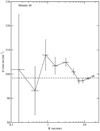 |
Fig. 13. Stellar surface density as a function of distance from the cluster centre. We note that the star counts in the innermost bins are affected by the bright saturated star. The dotted horizontal line indicates the adopted value for the background. We measure a cluster radius r = 6′±1′. |
Given that the quality of the Gaia photometry may be substantially degraded in the crowded inner regions of GCs, especially those located in the Galactic bulge, a significant fraction of stars in the inner region Minni 48 present missing values of BP and/or RP bands. This also leads the radial density profile to dive below the stellar background level in its inner bin. This effect is absent in the cluster outskirts, as shown in Fig. 13 and previously predicted by Riello et al. (2018). We argue that, except for the cluster core, the radial density profile is consistent with that of a GC, including the cluster radius of 6 ± 1′ suggested by Fig. 13.
The angular size of this GC is estimated to be r ∼ 6′±1′, equivalent to r ∼ 14 ± 2 pc at the distance of the bulge, a size that is comparable to those of other typical GCs. We note that this size should be taken as a rough estimate, given the difficulties in obtaining the surface density profile.
3.6. Measurement of total luminosity
The total absolute magnitude (luminosity) of Minni 48 is estimated to be MKs = −9.04 ± 0.66 mag, adopting a distance of D = 8.4 kpc. This value was measured by co-adding all bright cluster stars in the decontaminated near-IR CMD within 5′ of the GC centre. This is equivalent to MV = −6.5 ± 0.8 mag, assuming a typical GC colour of (V − Ks) ≈ 2.5 ± 0.5 mag. However, we stress that this estimated value is a lower limit, because of the contamination from the bright saturated star that does not allow us to count the central GC members. Finally, we would also like to highlight the difficulties in the size determination if the bright star causes a shift in the determination of the centroid of the stellar density.
As a consistency check on the luminosity, this cluster appears to be quite bright in the GLIMPSE and WISE images. In particular, the WISE image of Minni 48 (Fig. 3) resembles those of the known metal-rich bulge GCs, appearing somewhat brighter than NGC 6528 (D = 7.9 kpc, MV = −6.57 mag), and also slightly fainter than NGC 6553 (D = 6.8 kpc, MV = −7.77 mag).
At first sight it may seem surprising that a moderately cluster like this was missed before. However, there are two other examples of similar GCs recently discovered at very low latitudes under similar circumstances: FSR 1758 (Cantat-Gaudin et al. 2018; Barbá et al. 2019), and VVV-CL160 (Borissova et al. 2014; Minniti et al. 2021a). The first one is a much larger and brighter GC (Mi < −8.6 mag, r > 15′) that has been recently characterized using similar Gaia, VVV and DECaPS data (Barbá et al. 2019), and confirmed spectroscopically (Villanova 2019). The second example is a GC that has MK = −7.6, equivalent to MV = −5.1, and it is nearby (D = 4.2 kpc) and extended (Rt = 52′), but it is invisible in the optical images, while being barely visible in the near-IR images. This GC was clearly seen thanks only to the Gaia EDR3 and VVV PMs that allowed us to discriminate the field population (Minniti et al. 2021a).
3.7. Radial velocities
There are no radial velocities (RVs) available for obvious stellar sources associated with this GC. Unfortunately, most of its member stars are fainter than the limit of Gaia spectroscopy, which is G ≈ 15 mag. Ground-based follow-up spectroscopic observations are certainly needed. Future surveys such as 4MOST (Chiappini et al. 2019; Bensby et al. 2019) would be able to easily reach the GC member giants, thus providing accurate RVs. The final GC parameters adopted here are summarized in Table 1.
Summary of the derived physical parameters for Minni 48.
4. The RR Lyrae puzzle
Minniti et al. (2018) singled out this cluster as a metal-poor GC candidate because of an apparent (∼2σ) excess of RR Lyrae stars in this field. Table A.1 lists all RR Lyrae within 8′ of the GC, compiled from the OGLE (Soszyński et al. 2014), VVV (Majaess et al. 2018) and Gaia (Clementini et al. 2019) catalogues. The top panel of Fig. 2 shows the location of RR Lyrae in the zoomed 9′×7′ JHKs image centred on Minni 48. The white arrows point to the RR Lyrae stars in the field and the yellow arrow to a Type 2 Cepheid (WVir type; Soszyński et al. 2017).
Navarro et al. (2021) recently compiled all the bulge RR Lyrae variable stars from different surveys in order to study their spatial distribution. Figure 14 shows the distribution of distance moduli for all bulge RR Lyrae stars (grey histogram), compared with the RR Lyrae located within 3′ and 5′ of the cluster centre (purple and green histograms, respectively). These distance moduli were computed following the procedure described by Minniti et al. (2017b) and Palma et al. (2019). The black arrow indicates the adopted GC distance modulus m − M = 14.61 mag, for reference. As expected, the distance distribution for all RR Lyrae is centred at a distance modulus of 14.5 mag, being very broad (grey histogram) due to the depth of the bulge along the line of sight. The distances for the RR Lyrae stars in the GC field are consistent with that of Minni 48, although their Gaia EDR3 PMs are more scattered than those of the GC members as shown in Fig. 14. That can be due, however, to the low luminosity of these objects. We also note, as a consistency argument, that adopting a much closer distance to these objects would lead to a very high reddening that would be inconsistent with the existing reddening maps.
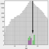 |
Fig. 14. Distribution of distance moduli for all bulge RR Lyrae stars from the OGLE, VVV, and Gaia catalogues (grey histogram), compared with the RR Lyrae stars located within 3′ and 5′ of the cluster centre (purple and green histograms, respectively). The black arrow indicates the adopted GC distance modulus for reference. |
On the basis of our confirmation of Minni 48 as a metal-rich bulge cluster (based on the statistical decontamination of the optical and near-IR CMDs), these RR Lyrae stars are probably mere field objects and not cluster members, since RR Lyrae stars in metal-rich GCs are very rare. The RR Lyrae appear to have a more extended distribution than that of the reddest giants that are clearly more clustered (Fig. 9), and their PMs are also do not appear to be very clustered (Fig. 15). However, follow-up observations (especially measurements of RVs) of these objects are needed in order to confirm or discard cluster membership. We tentatively conclude that these RR Lyrae are field objects because the GC is metal-rich, their PM distribution is not very concentrated, and they exhibit a wide distance distribution. However, we cannot definitely discard the presence of two stellar populations, nor that a couple of RR Lyrae may still be associated with the cluster.
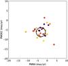 |
Fig. 15. Vector PM diagram for all bulge RR Lyrae stars from the OGLE, VVV, and Gaia catalogues located within 10′ of the cluster centre. The scale is the same as in Fig. 9, and the RR Lyrae are colour-coded with distance from the GC centre, with the darkest objects being closer to the centre and the lighter ones being farther away. The black circle is centred on the mean GC PM for comparison. |
Minni 48 is certainly a very puzzling GC because in the optical Gaia CMD of this region there are two well-separated RGBs (Fig. 1). On one hand, the conspicuous RC and the redder GB seen in the near-IR data, added to the presence of very bright red stars in the WISE data, support a very metal-rich component. On the other hand, the presence of RR Lyrae stars and the bluer GB suggest also the existence of a metal-poor population component.
The findings, however puzzling, are very interesting as the cluster region appears to contain a double population: a metal-rich old component with [Fe/H] = − 0.2 dex, and a metal-poor old component with [Fe/H] ∼ − 1.3 dex. If these results are confirmed spectroscopically not to be simply the effect of field stars contamination and the RR Lyrae stars are metal-poor cluster members, we may be either in the presence of the remaining nucleus of an accreted dwarf galaxy that originally had a composite population, or the final product of a merger between a metal-poor and a metal-rich cluster. In both regards, this is a very interesting object to be followed-up spectroscopically.
We also note that there is a planetary nebula/symbiotic star candidate (PN Th 3-30; Mikolajewska et al. 1997), located about 6′ away from the cluster centre. This is also worth noticing because planetary nebulae that are GC members are certainly very rare (Jacoby et al. 1997; Minniti et al. 2019). Nevertheless, the association of this planetary nebula with Minni 48 in this crowded field also needs to be confirmed spectroscopically.
5. Summary and conclusions
We analysed optical and near-IR photometry of the candidate GC Minni 48, which was recently discovered using the VVV survey. The cluster field contains a bright foreground star, so multi-colour photometric data were needed in order to confirm its real GC nature, as well as to determine its physical parameters.
We measured the cluster’s fundamental parameters, including reddening, extinction, distance, metallicity, age, radius, and luminosity. Our main results for Minni 48 are listed in Table 1. These parameters are consistent with a luminous metal-rich GC, located at a projected angular distance of about 0.4 kpc from the Galactic centre. We emphasize that the Minni 48 analysis was conducted by using multiple photometry and a set of filters and decontamination procedures and that the GC evolutionary sequences survived in all procedures. A field fluctuation is unlikely to survive such a set of well-established tools. Therefore, Minni 48 joins the MW GC system as another genuine GC in the inner bulge.
Unfortunately, as a bulge GC, Minni 48 accumulates a set of Gaia data limitations, such as bright stars in the projected neighbourhood and crowding effects within the GC core and the Galactic bulge, which significantly reduce the known gain provided by Gaia in star cluster analysis. Thus, deeper photometry is required to uncover the cluster core, but out of the core a prominent cluster can be seen. We also measure a cluster radius of 6 ± 1′, which is consistent with the typical sizes of Galactic GCs.
This is a very interesting bulge GC to follow up on with more detailed observations. Despite the statistically decontaminated CMDs yielding only a metal-rich population, we cannot ignore the detection of a significant metal-poor stellar component in this field. In particular, we also point out the presence of RR Lyrae variable stars in the field that need to be followed up on spectroscopically in order to confirm or discard their cluster membership.
Acknowledgments
We gratefully acknowledge data from the ESO Public Survey program ID 179.B-2002 and 198.B-2004 taken with the VISTA telescope, and products from the Cambridge Astronomical Survey Unit (CASU). This publication makes use of data products from the WISE satellite, which is a joint project of the University of California, Los Angeles, and the Jet Propulsion Laboratory/California Institute of Technology, funded by the National Aeronautics and Space Administration. This research has made use of NASA’s Astrophysics Data System Bibliographic Services and the SIMBAD database operated at CDS, Strasbourg, France, and the Two Micron All Sky Survey (2MASS), and the Gaia-DR2 and EDR3. D. M. is supported by the BASAL Center for Astrophysics and Associated Technologies (CATA) AF B-170002, and by FONDECYT Regular grant No. 1170121. J. A.-G. acknowledges support from Fondecyt Regular 1201490 and from ANID – Millennium Science Initiative Program – ICN12_009 awarded to the Millennium Institute of Astrophysics MAS. R.K.S. acknowledges support from CNPq/Brazil through project 305902/2019-9. T. P. and J. J. C. acknowledge support from the Argentinian institutions CONICET and SECYT (Universidad Nacional de Córdoba).
References
- Alonso-García, J., Dekany, I., Catelan, M., et al. 2015, AJ, 149, 99 [NASA ADS] [CrossRef] [Google Scholar]
- Alonso-García, J., Minniti, D., Catelan, M., et al. 2017, ApJ, 849, L13 [Google Scholar]
- Alonso-García, J., Saito, R. K., Hempel, M., et al. 2018, A&A, 619, A4 [NASA ADS] [CrossRef] [EDP Sciences] [Google Scholar]
- Arenou, F., Luri, X., Babusiaux, C., et al. 2018, A&A, 616, A17 [NASA ADS] [CrossRef] [EDP Sciences] [Google Scholar]
- Bailer-Jones, C. A. L., Rybizki, J., Fouesneau, M., Mantelet, G., & Andrae, R. 2018, AJ, 156, 58 [NASA ADS] [CrossRef] [Google Scholar]
- Barbá, R., Minniti, D., Geisler, D., et al. 2019, ApJ, 870, L24 [NASA ADS] [CrossRef] [Google Scholar]
- Benjamin, R. A., Churchwell, E., Babler, B. L., et al. 2003, PASP, 115, 953 [NASA ADS] [CrossRef] [Google Scholar]
- Bensby, T., Feltzing, S., Gould, A., et al. 2017, A&A, 605, A89 [NASA ADS] [CrossRef] [EDP Sciences] [Google Scholar]
- Bensby, T., Bergemann, M., Rybizki, J., et al. 2019, ESO Messenger, 175, 35 [NASA ADS] [Google Scholar]
- Bernard, E., Schultheis, M., Di Matteo, P., et al. 2018, MNRAS, 477, 3507 [NASA ADS] [CrossRef] [Google Scholar]
- Bica, E., Bonatto, C., & Camargo, D. 2008, MNRAS, 385, 349 [NASA ADS] [CrossRef] [Google Scholar]
- Bonatto, C., & Bica, E. 2007, MNRAS, 477, 1301 [NASA ADS] [CrossRef] [Google Scholar]
- Borissova, J., Chené, A.-N., Ramírez Alegría, S., et al. 2014, A&A, 569, 24 [Google Scholar]
- Bressan, A., Marigo, P., Girardi, L., et al. 2012, MNRAS, 427, 127 [NASA ADS] [CrossRef] [Google Scholar]
- Camargo, D. 2018, ApJ, 860, L27 [Google Scholar]
- Camargo, D., & Minniti, D. 2019, MNRAS, 484, 90 [Google Scholar]
- Camargo, D., Bonatto, C., & Bica, E. 2009, A&A, 508, 211 [NASA ADS] [CrossRef] [EDP Sciences] [Google Scholar]
- Camargo, D., Bica, E., & Bonatto, C. 2015, New Astron., 34, 84 [NASA ADS] [CrossRef] [Google Scholar]
- Camargo, D., Bica, E., & Bonatto, C. 2016, MNRAS, 455, 3126 [Google Scholar]
- Cantat-Gaudin, T., Jordi, C., Vallenari, A., et al. 2018, A&A, 618, A93 [NASA ADS] [CrossRef] [EDP Sciences] [Google Scholar]
- Cardelli, J. A., Clayton, G. C., & Mathis, J. S. 1989, ApJ, 345, 245 [NASA ADS] [CrossRef] [Google Scholar]
- Cassisi, S., & Salaris, M. 1997, MNRAS, 285, 593 [NASA ADS] [Google Scholar]
- Chen, B. Q., Schultheis, M., Jiang, B. W., et al. 2013, A&A, 550, A42 [NASA ADS] [CrossRef] [EDP Sciences] [Google Scholar]
- Chiappini, C., Minchev, I., Starkenburg, E., et al. 2019, ESO Messenger, 175, 30 [NASA ADS] [Google Scholar]
- Churchwell, E., Babler, B. L., Meade, M. R., et al. 2009, PASP, 121, 213 [NASA ADS] [CrossRef] [Google Scholar]
- Clementini, G., Ripepi, V., Molinaro, R., et al. 2019, A&A, 622, A60 [NASA ADS] [CrossRef] [EDP Sciences] [Google Scholar]
- Cohen, R. E., Moni Bidin, C., Mauro, F., et al. 2017, MNRAS, 464, 1874 [Google Scholar]
- Cutri, R. M., Skrutskie, M. F., van Dyk, S., et al. 2003, VizieR Online Data Catalogue: II/246 [Google Scholar]
- Dotter, A., Sarajedini, A., Anderson, J., et al. 2010, ApJ, 708, 698 [NASA ADS] [CrossRef] [Google Scholar]
- Evans, D. W., Riello, M., De Angeli, F., et al. 2018, A&A, 616, A4 [NASA ADS] [CrossRef] [EDP Sciences] [Google Scholar]
- Gaia Collaboration (Brown, A. G. A., et al.) 2018a, A&A, 616, A1 [NASA ADS] [CrossRef] [EDP Sciences] [Google Scholar]
- Gaia Collaboration (Mignard, F., et al.) 2018b, A&A, 616, A14 [NASA ADS] [CrossRef] [EDP Sciences] [Google Scholar]
- Gaia Collaboration (Brown, A. G. A., et al.) 2021, A&A, 649, A1 [NASA ADS] [CrossRef] [EDP Sciences] [Google Scholar]
- Geisler, D., Villanova, S., O’Connell, J. E., et al. 2021, A&A, in press, https://doi.org/10.1051/0004-6361/202140436 [Google Scholar]
- Girardi, L. 2016, ARA&A, 54, 95 [NASA ADS] [CrossRef] [EDP Sciences] [Google Scholar]
- Gonzalez, O. A., Rejkuba, M., Minniti, D., et al. 2011, A&A, 534, L14 [NASA ADS] [CrossRef] [EDP Sciences] [Google Scholar]
- González-Fernández, C., Hodgkin, S. T., Irwin, M. J., et al. 2018, MNRAS, 474, 5459 [Google Scholar]
- Hajdu, G., Dekany, I., Catelan, M., & Grebel, E. K. 2020, Exp. A., 49, 217 [NASA ADS] [Google Scholar]
- Haywood, M., Di Matteo, P., Snaith, O., & Calamida, A. 2016, A&A, 593, A82 [NASA ADS] [CrossRef] [EDP Sciences] [Google Scholar]
- Irwin, M. J., Lewis, J., Hodgkin, S., et al. 2004, Proc. SPIE, 5493, 411 [NASA ADS] [CrossRef] [Google Scholar]
- Jacoby, G. H., Morse, J. A., Fullton, L. K., Kwitter, K. B., & Henry, R. B. C. 1997, AJ, 114, 2611 [NASA ADS] [CrossRef] [Google Scholar]
- Koposov, S. E., Belokurov, E., & Torrealba, G. 2017, MNRAS, 470, 2702 [NASA ADS] [CrossRef] [Google Scholar]
- Lewis, J. R., Irwin, M., & Bunclark, P. 2010, Astronomical Data Analysis Software and Systems XIX, 434, 91 [NASA ADS] [Google Scholar]
- Longmore, A. J., Kurtev, R., Lucas, P. W., et al. 2011, MNRAS, 416, L465 [NASA ADS] [Google Scholar]
- Majaess, D., Dekany, I., Hajdu, G., et al. 2016, Ap&SS, 363, 127 [Google Scholar]
- Majaess, D., Turner, D., Dekany, I., et al. 2018, A&A, 593, 124 [Google Scholar]
- Mauro, F., Moni Bidin, C., Chene, A.-N., et al. 2013, RMxAA, 49, 189 [NASA ADS] [Google Scholar]
- Mikolajewska, J., Acker, A., & Stenholm, B. 1997, A&A, 327, 191 [NASA ADS] [Google Scholar]
- Minniti, D., Lucas, P. W., Emerson, J. P., et al. 2010, New Astron., 15, 433 [Google Scholar]
- Minniti, D., Hempel, M., Toledo, I., et al. 2011, A&A, 527, A81 [NASA ADS] [CrossRef] [EDP Sciences] [Google Scholar]
- Minniti, D., Geisler, D., Alonso-García, J., et al. 2017a, ApJ, 849, L24 [NASA ADS] [CrossRef] [Google Scholar]
- Minniti, D., Palma, T., Dekany, I., et al. 2017b, ApJ, 838, L14 [NASA ADS] [CrossRef] [Google Scholar]
- Minniti, D., Alonso-García, J., & Pullen, J. B. 2018, RNAAS, 1, 54 [NASA ADS] [Google Scholar]
- Minniti, D., Dias, B., Gómez, M., Palma, T., & Pullen, J. B. 2019, ApJ, 884, L15 [CrossRef] [Google Scholar]
- Minniti, D., Fernandez-Trincado, J., Gomez, M., et al. 2021a, A&A, 650, L11 [NASA ADS] [CrossRef] [EDP Sciences] [Google Scholar]
- Minniti, D., Fernández-Trincado, J. G., Smith, L. C., et al. 2021b, A&A, 648, A86 [NASA ADS] [CrossRef] [EDP Sciences] [Google Scholar]
- Moni-Bidin, C., Mauro, F., Geisler, D., et al. 2011, A&A, 535, A33 [NASA ADS] [CrossRef] [EDP Sciences] [Google Scholar]
- Nataf, D. M., Gonzalez, O. A., Casagrande, L., et al. 2016, MNRAS, 456, 2692 [NASA ADS] [CrossRef] [Google Scholar]
- Navarro, G., Minniti, D., Capuzzo-Dolcetta, R., et al. 2021, A&A, 646, A45 [EDP Sciences] [Google Scholar]
- Nishiyama, S., Tamura, M., Hatano, H., et al. 2009, ApJ, 696, 1407 [NASA ADS] [CrossRef] [Google Scholar]
- Ortolani, S., Bonatto, C., Bica, E., Barbuy, B., & Saito, R. K. 2012, AJ, 144, 147 [CrossRef] [Google Scholar]
- Palma, T., Minniti, D., Dekany, I., et al. 2016, New Astron., 49, 50 [CrossRef] [Google Scholar]
- Palma, T., Minniti, D., Alonso-García, J., et al. 2019, MNRAS, 487, 3140 [Google Scholar]
- Piatti, A. E. 2018, MNRAS, 477, 2164 [Google Scholar]
- Riello, M., De Angeli, F., Evans, D. W., et al. 2018, A&A, 616, A3 [NASA ADS] [CrossRef] [EDP Sciences] [Google Scholar]
- Ruiz-Dern, L., Babusiaux, C., Arenou, F., Turon, C., & Lallement, R. 2018, A&A, 609, A116 [NASA ADS] [CrossRef] [EDP Sciences] [Google Scholar]
- Ryu, J., & Lee, M. G. 2018, ApJ, 863, 38 [NASA ADS] [CrossRef] [Google Scholar]
- Saito, R. K., Hempel, M., Minniti, D., et al. 2012, A&A, 537, A107 [NASA ADS] [CrossRef] [EDP Sciences] [Google Scholar]
- Schlafly, E. F., & Finkbeiner, D. P. 2011, ApJ, 737, 103 [NASA ADS] [CrossRef] [Google Scholar]
- Schlafly, E. F., Green, G. M., Lang, D., et al. 2017, ApJS, 234, 39 [Google Scholar]
- Serenelli, A., Weiss, A., Cassisi, S., Salaris, M., & Pietrinferni, A. 2017, A&A, 606, A33 [NASA ADS] [CrossRef] [EDP Sciences] [Google Scholar]
- Skrutskie, M. F., Cutri, R. M., Stiening, R., et al. 2006, AJ, 131, 1163 [NASA ADS] [CrossRef] [Google Scholar]
- Soszyński, I., Udalski, A., Szymanski, M. K., et al. 2014, Acta Astron., 64, 177 [Google Scholar]
- Soszyński, I., Udalski, A., Szymanski, M. K., et al. 2017, Acta Astron., 67, 297 [Google Scholar]
- Soto, M., Barbá, R., Gunthardt, G., et al. 2013, A&A, 552, A101 [NASA ADS] [CrossRef] [EDP Sciences] [Google Scholar]
- Surot, F., Valenti, E., Gonzalez, O. A., et al. 2020, A&A, 644, A140 [CrossRef] [EDP Sciences] [Google Scholar]
- Valenti, E., Ferraro, F. R., & Origlia, L. 2007, AJ, 133, 1287 [NASA ADS] [CrossRef] [Google Scholar]
- Villanova, S., Monaco, L., Geisler, D., et al. 2019, ApJ, 882, 174V [Google Scholar]
- Wright, E. L., Eisenhardt, P. R. M., & Mainzer, A. K. 2010, AJ, 140, 1868 [NASA ADS] [CrossRef] [Google Scholar]
Appendix A: Additional table
Table A.1 below lists the data for all the known RR Lyrae variable stars in the cluster field (within 8′). We give the IDs, periods in days, distances from the cluster centre in arcminutes, positions in equatorial coordinates (J2000), optical and near-IR magnitudes from OGLE and VVV, respectively, and RR Lyrae types.
Photometry of the RR Lyrae variables in the cluster field (within 8′).
All Tables
All Figures
|
Fig. 1. Gaia EDR3 optical CMD (G vs. BP–RP) for a r < 3′ region centred in the GC. This CMD shows that the upper RGB in this area is clearly split into a bluer and a redder component. |
| In the text | |
|
Fig. 2. Zoomed-in views of a 9′×7′ region centred on Minni 48 obtained with VVV (top panel), 2MASS (middle panel), and DECaPS (bottom panel) This figure is oriented along equatorial coordinates, with east to the left and north to the top (see also Fig. 3). The white arrows point to the RR Lyrae stars and the yellow arrow to the Type 2 Cepheid. The saturated star near the centre is the bright source IRAS 17302-2800, with Ks = 3.33 and (J − Ks) = 1.81 mag. |
| In the text | |
|
Fig. 3. Near and mid-IR views of the new GC. Top: wide field JHKs mosaic covering the VVV tiles b359 to b361, showing the positions of Minni 48 compared with those of the two well-known GCs: HP 1 and Terzan 2. This field, covering approximately 1.5° ×4°, is oriented along Galactic coordinates, with longitudes increasing to the left and latitudes to the top. Bottom: zoomed-in view of a 20′×20′ region centred on Minni 48 obtained with WISE in the mid-IR (3.6–8 microns). There is a clear concentration of bright IR stars in the cluster core. The white box shows the location of the zoomed-in images portrayed in Fig. 2. |
| In the text | |
|
Fig. 4. Map of WISE sources (left panel) and a WISE mid-IR CMD (right panel). There is a clear concentration of many RGs in the cluster core. The brightest IR stars are indicated with blue circles. The brightest star, with W1 = 2.1, W1 − W2 = 0 mag, is the foreground source IRAS 17302-2800, which is located close to the cluster centre. For comparison, the region where the Gaia-EDR3 CMD of Fig. 1 is made (r < 3′) is the inner red region shown in this map. |
| In the text | |
|
Fig. 5. Gaia EDR3 optical CMDs (G vs. BP-RP) for the GC region (left panel), a background region (middle panel), and the statistically decontaminated region following Camargo et al. (2009; right panel). The last CMD clearly shows that only the RGB (more metal rich) survives the decontamination procedure. The Gaia decontaminated CMD is fitted by a PARSEC isochrone with age 10 Gyr and metallicity [Fe/H] = − 0.2 dex. |
| In the text | |
|
Fig. 6. 2MASS near-IR CMDs (Ks vs. J − Ks) for the GC region (left panel), a background region (middle panel), and the statistically decontaminated region following Camargo et al. (2009; right panel). The last CMD clearly shows a tight metal-rich RGB and the RGB tip at Ks = 7.75 ± 0.10 mag. The red line shows a PARSEC isochrone of age 10 Gyr and metallicity [Fe/H] = − 0.2 dex. |
| In the text | |
|
Fig. 7. Deep VVV near-IR CMDs (Ks vs. J − Ks) for the GC region (left panel), a background region (middle panel), and the statistically decontaminated region following Palma et al. (2019; right panel). The last CMD clearly shows the GC RC at Ks = 13.45 mag. |
| In the text | |
|
Fig. 8. Optical CMDs within 3′ of the GC centre using the DECaPS survey (Schlafly et al. 2017). These diagrams clearly show the GC RC at r = 18.65 and i = 17.50 mag. |
| In the text | |
|
Fig. 9. Gaia-EDR3 vector PM diagrams for the whole 20′ field (left panel) compared with a 5′ field centred on the cluster (right panel) and with an equal area field located 10′ south of the cluster (middle panel). |
| In the text | |
|
Fig. 10. Optical and near-IR CMDs for the GC region after the PM decontamination using Gaia EDR3 data. |
| In the text | |
|
Fig. 11. Optical and near-IR CMD luminosity functions (in blue and red, respectively) for the GC region after the PM decontamination using Gaia EDR3 data. |
| In the text | |
|
Fig. 12. Gaia-EDR3 PM distribution. The black circles are the stars in the central region of Minni 48 (errors < 0.3 mas yr−1), while the brown circles represent stars located in a ring in the surrounding field. |
| In the text | |
|
Fig. 13. Stellar surface density as a function of distance from the cluster centre. We note that the star counts in the innermost bins are affected by the bright saturated star. The dotted horizontal line indicates the adopted value for the background. We measure a cluster radius r = 6′±1′. |
| In the text | |
|
Fig. 14. Distribution of distance moduli for all bulge RR Lyrae stars from the OGLE, VVV, and Gaia catalogues (grey histogram), compared with the RR Lyrae stars located within 3′ and 5′ of the cluster centre (purple and green histograms, respectively). The black arrow indicates the adopted GC distance modulus for reference. |
| In the text | |
|
Fig. 15. Vector PM diagram for all bulge RR Lyrae stars from the OGLE, VVV, and Gaia catalogues located within 10′ of the cluster centre. The scale is the same as in Fig. 9, and the RR Lyrae are colour-coded with distance from the GC centre, with the darkest objects being closer to the centre and the lighter ones being farther away. The black circle is centred on the mean GC PM for comparison. |
| In the text | |
Current usage metrics show cumulative count of Article Views (full-text article views including HTML views, PDF and ePub downloads, according to the available data) and Abstracts Views on Vision4Press platform.
Data correspond to usage on the plateform after 2015. The current usage metrics is available 48-96 hours after online publication and is updated daily on week days.
Initial download of the metrics may take a while.