| Issue |
A&A
Volume 652, August 2021
|
|
|---|---|---|
| Article Number | A134 | |
| Number of page(s) | 11 | |
| Section | Extragalactic astronomy | |
| DOI | https://doi.org/10.1051/0004-6361/202039859 | |
| Published online | 24 August 2021 | |
Merging timescale for the supermassive black hole binary in interacting galaxy NGC 6240
1
Main Astronomical Observatory, National Academy of Sciences of Ukraine, 27 Akademika Zabolotnoho St., 03143 Kyiv, Ukraine
e-mail: sobolenko@mao.kiev.ua
2
National Astronomical Observatories and Key Laboratory of Computational Astrophysics, Chinese Academy of Sciences, 20A Datun Rd., Chaoyang District, 100101 Beijing, PR China
3
Astronomisches Rechen-Institut, Zentrum für Astronomie, University of Heidelberg, Mönchhofstrasse 12-14, 69120 Heidelberg, Germany
4
Kavli Institute for Astronomy and Astrophysics, Peking University, Yiheyuan Lu 5, Haidian Qu, 100871 Beijing, PR China
Received:
5
November
2020
Accepted:
10
May
2021
Context. One of the mechanisms leading to the creation of a supermassive black hole (SMBH) is the so-called hierarchical merging scenario. Central SMBHs at the final phase of interacting and coalescing host-galaxies are observed as SMBH binary (SMBHB) candidates at different separations from hundreds of parsecs to megaparsecs.
Aims. Today one of the strongest SMBHB candidates is the ultraluminous infrared galaxy NGC 6240 which was spatially and spectroscopically resolved in X-rays by Chandra. Dynamical calculation of central SMBHBs merging in a dense stellar environment allows us to retrace their evolution from kiloparsec to megaparsec scales. The main goal of our dynamical modeling was to reach the final, gravitational wave emission regime for the model BHs.
Methods. We present direct N-body simulations with up to one million particles and relativistic post-Newtonian corrections for the SMBH particles up to 3.5 post-Newtonian terms.
Results. Generally speaking, the set of initial physical conditions can strongly affect our merging time estimations. However, within a certain range of our parameters, we do not find any strong correlation between merging time and BH-to-BH mass or BH-to-bulge mass ratios. Varying the numerical parameters (like particle number – N) does not significantly change the merging time limits. From our 20 models, we find an upper limit on the merging time for central SMBHBs of less than ∼55 Myr. This precise number is only valid for our combination of initial mass ratios.
Conclusions. Further detailed research of rare dual and multiple BHs in dense stellar environments (based on observational data) could clarify the dynamical co-evolution of central BHs and their host-galaxies.
Key words: black hole physics / gravitational waves / galaxies: kinematics and dynamics / galaxies: nuclei / galaxies: individual: NGC 6240 / methods: numerical
© ESO 2021
1. Introduction
The majority of classical bulges and elliptical galaxies harbor central supermassive black holes (SMBHs) and even a portion (< 20%) of dwarf galaxies probably contain them (Kormendy & Ho 2013; Mezcua 2017). The SMBH with a mass of M = 4.28 × 10⁶ M⊙ (Gillessen et al. 2017) at the center of the Milky Way is powerful evidence of this. Theoretically, SMBHs can grow to observable masses (106–1010 M⊙) in different ways. One of the possible mechanisms for SMBH formation is through a hierarchical merging of host galaxies according to the standard ΛCDM cosmology (White & Rees 1978). Co-evolution of SMBHs and galaxies takes place via strong correlations between the SMBH mass and the parameters of galaxy bulges (velocity dispersion, bulge luminosity/mass, etc.; Kormendy & Ho 2013) or via the strong correlation between SMBH mass and global star formation properties in the host galaxies (Chen et al. 2020). Competing route of the SMBHs formation is production in starburst clusters formed at the onset of the formation of their hosting galaxy (Kroupa et al. 2020).
From observations, we expect to find SMBHs at different merging stages with a detection of strong gravitational wave (GW) emission at the last phase of coalescence. Observations at nanohertz frequencies (∼1–100 nHz) accessible to pulsar timing arrays (PTAs; Sesana et al. 2008; Burke-Spolaor et al. 2019) predict the detection of non-oscillatory components of GW signals for SMBH binary (SMBHB) coalescence at the high end of the mass distribution in the next 5–10 yrs (Taylor et al. 2019). Gravitational waves from super-massive (< 107 M⊙) and intermediate mass BHs could be directly detected by the Laser Interferometer Space Antenna (LISA) space mission (Amaro Seoane 2013) before 2030.
Dynamical evolution of SMBHBs in dense stellar environments (gas-free, so-called dry merging) consists of three main parts (Begelman et al. 1980). In the first stage, the central BHs are surrounded by stars approaching via efficient dynamical friction. Assuming the galaxy center density distribution as a singular isothermal sphere, the central BHs each with masses m• are sinking toward the center of the stellar distribution, containing N stars, with the density  at the timescale:
![$$ \begin{aligned} \tau _{\rm df} \sim 2\times 10^{8}{\frac{1}{\mathrm{ln}(N)}}~\Bigl (\frac{10^{6}\; M_{\odot }}{m_{\bullet }}\Bigr ) \Bigl (\frac{r_{c}}{100 \;\mathrm {pc}}\Bigr )^{2} \Bigl (\frac{\sigma }{100 \;\mathrm {km}\,\mathrm {s}^{-1}}\Bigr ) \; [\mathrm {yr}], \end{aligned} $$](/articles/aa/full_html/2021/08/aa39859-20/aa39859-20-eq2.gif)
where rc is a core radius, σ is a velocity dispersion, and G is the gravitational constant (Yu 2002). Black holes at this stage are effectively losing energy and form a bound pair with a semimajor axis ab which is almost equal to their influence radius.
SMBHs continue to in-spiral toward each other due to decreasing dynamical friction. By definition, the influence radius is the radius that contains as much as twice the mass of the central SMBHB M• = m•1 + m•2, where the primary BH mass m•1 is bigger than the secondary BH mass m•2. Furthermore, three-body interactions (scattering) with passing stars become dominant and the second phase starts when the binary semimajor axis reaches a value of ah ≡ Gμ/4σ2, where μ = m•1m•2/(m•1 + m•2) is a reduced mass (Quinlan 1996; Yu 2002). A binary with a semimajor axis a is effectively hardening over a timescale of:
![$$ \begin{aligned} \tau _{\rm hard} \sim 70\ \Bigl (\frac{\sigma }{100\; \mathrm {km} \;\mathrm {s}^{-1}}\Bigr )\Bigl (\frac{10^{4}\; M_{\odot } \;\mathrm{pc}^{-3}}{\rho }\Bigr ) \Bigl (\frac{10^{-3} \; \mathrm{pc}}{a}\Bigr ) \; [\mathrm {Myr}]. \end{aligned} $$](/articles/aa/full_html/2021/08/aa39859-20/aa39859-20-eq3.gif)
In the final stage, the GW radiation can effectively carry the binary kinetic energy and angular momentum away. Assuming the simple post-Newtonian (PN) formalism, and using only the 2.5 PN corrections, the GW merging timescale for the binary with eccentricity e can be described as:
![$$ \begin{aligned} \tau _{\rm gw} = \frac{5}{64} \frac{c^{5}a^{4}}{G^{3}\mu M_{\bullet }^{2}}\frac{(1-e^{2})^{7/2}}{1+73e^{2}/24+37e^{4}/96}\;[\mathrm {s}] , \end{aligned} $$](/articles/aa/full_html/2021/08/aa39859-20/aa39859-20-eq4.gif)
where c is the speed of light and M• is the total mass of the BHs (Peters & Mathews 1963; Peters 1964a,b). In this final merging stage, the binary lifetime rapidly decreases and the orbits begin to circularize. During this final merging stage a “recoil” can take place with a speed of up to 5000 km s−1 (Peres 1962; Bekenstein 1973; Lousto & Healy 2019).
The scenario and timescales described above simply show the principal evolutionary path. The timescale for transition from one phase to another remains uncertain. As an example, in the case of an extreme mass ratio m•2/m•1 ≪ 1, the GW radiation can start to dominate in dissipation before the strong hardening phase begins (Yu 2002). Also, the well-known “final parsec problem” can even stall the SMBHB orbital evolution and significantly increase the coalescence time to more than a Hubble time (Milosavljević & Merritt 2001; Milosavljević et al. 2003). In a gas-free ideal stellar spherical system, a depletion of the loss-cone is quite possible, when there are not enough stars for the energy and angular momentum to be dissipated. However, numerical simulations applying a triaxial geometry based on the observed merging remnants with a sufficient rate of non-axisymmetry have shown that hardening of the BHs does not stall (Berczik et al. 2006; Gualandris et al. 2017).
The presence of gas (gas-rich, so-called wet merging) influences the timescales of the different merging phases and can offer a further solution for the final parsec problem. Mayer et al. (2007) first showed the evolution of BHs in gas-rich mergers from tens of kiloparsecs (kpc) to several megaparsecs (mpc) on timescales of around 5 Gyr. A variety of studies have shown the complex and different roles of gas in minor (mass ratio ≤10) and major mergers (mass ratio > 10): gas can both accelerate the shrinking of the binary orbit and delay its evolution. In major mergers, BHs are pairing and binary is hardening due to the effects of the post-merger gas disk (Escala et al. 2005; Cuadra et al. 2009; Souza Lima et al. 2020) and interaction of gas clumps with the binary (Goicovic et al. 2017, 2018). The role of gas in minor mergers strongly depends on initial geometry and gas content (Callegari et al. 2009, 2011). For heavy SMBHBs (with BH mass ratios of ∼1 and masses of more than 107 M⊙) gas disks affect the merging processes at a significantly lower rate (Cuadra et al. 2009; Lodato et al. 2009). One simulation (Khan et al. 2016) showed ab-initio SMBHB evolution starting from a cosmological simulation to GW emission.
As mentioned above, we should observe SMBH coalescence at different merging stages: such as double active galactic nuclei (AGNs, at separations from tens of kpc to kpc scale), SMBHBs (at separations from pc to subpc scale), and recoiling BHs. The interacting galaxy NGC 6240 was the first directly detected (X-ray spectroscopy and image confirmation) and spatially resolved double-AGN candidate (Komossa et al. 2003). Some strong double-AGN candidates were serendipitously discovered (those with separations ΔR < 1 kpc are the most suitable for N-body simulations): 4C+37.11 (Maness et al. 2004; Rodriguez et al. 2006), SDSS J115822+323102 (Müller-Sánchez et al. 2015), NGC3393 (Fabbiano et al. 2011), IC4553 (Paggi et al. 2017), Mrk 273 (Vivian et al. 2013), and SDSS J132323-015941 (Woo et al. 2014). A systematic search gave samples of double-AGN candidates at optical (McGurk et al. 2011, 2015; Fu et al. 2012; Ellison et al. 2017), X-ray (usually previously selected from another band Green et al. 2011; Gross et al. 2019), infrared (Satyapal et al. 2017; Pfeifle et al. 2019) and radio (Burke-Spolaor 2011) bands, each of which requires a more detailed multi-wavelength investigation. Observing the spatial offset of SMBHs from their host galaxy stellar center or the broad emission-line velocity offset from the systematic velocity provided a dozen candidate recoiling SMBHs. The first such candidate was the luminous quasar SDSS J0927+2943 with an offset of ∼ 2650 km s−1 (Komossa et al. 2008). In our paper, for simplification, we use the term SMBHB regardless of the component separation.
The paper is structured in the following way. We describe the physical parameters of the galaxy NGC 6240 and central BHs that we use for N-body simulations in Sect. 2. How we construct the physical and numerical N-body models is detailed in Sect. 3. Our code is presented in Sect. 4. The motion of BHs as relativistic particles and their hardening is represented using post-Newtonian formalism in Sect. 5. We describe the evolution of merging BHs in Sect. 6 and summarize our results in Sect. 7.
2. NGC 6240 physical characteristics
As mentioned above, the first spatially resolved SMBHB is a system in the interacting galaxy NGC 6240 (z = 0.0243 Solomon et al. 1997) which was optically classified as a low-ionization nuclear emission-line region (LINER; Véron-Cetty & Véron 2006). Chandra observations confirmed the presence of two luminous hard X-ray emission sources at the south (S) and north (N) cores with a strong neutral Fe Kα line at each (Komossa et al. 2003) associated to BHs. Using the adaptive optics at the Keck II telescope (Max et al. 2007; Medling et al. 2011), a separation was found between the components of ∼1.5″ which corresponds to previous radio (Beswick et al. 2001; Gallimore & Beswick 2004) and X-ray observations (Komossa et al. 2003). Assuming a Hubble constant of H0 = 68 km s−1 Mpc−1 (Planck Collaboration XVI 2014) at the distance of NGC 6240 1″ corresponds to 500 pc, this scale respectively converts 1″.5 to 750 pc between the cores. Kollatschny et al. (2020) reported a third minor component S2 which was placed at 0.42″ (210 pc) from S1 (previous S) nuclei. Below, we use ‘S’ (S1+S2) to designate the south nucleus if we talk about the binary system, or ‘S1/S2’ when discussing the triple system.
Earlier CO(2-1) observations indicated a maximum gas concentration between the two nuclei. This was associated with the existence of a central thin disk (Tacconi et al. 1999). The latest ALMA observations confirm the presence of a nuclear molecular gas bulk of ∼9 × 10⁹ M⊙ within the ∼1″ (500 pc) between the two nuclei (Treister et al. 2020). The lesser part of the gas concentrated within the influence sphere of the BH at the N and S nuclei, ∼7.4 × 10⁸ M⊙ and ∼3.3 × 10⁹ M⊙ respectively. A velocity dispersion analysis links the presence of gas to an ongoing merging process rather than disk availability (Treister et al. 2020).
Based on X-ray luminosity (Engel et al. 2010), the combined BH (N+S) mass is 4 × 10⁸ M⊙. Certain assumptions of this method led to an uncertainty of at least a factor of a few. The central part of the S nucleus inside the sphere of influence of the BH was resolved using adaptive optics (Medling et al. 2011). Stellar dynamics gave limits for the S BH mass from 8.7 ± 0.3 × 10⁸ M⊙ to 2.0 ± 0.2 × 10⁹ M⊙. Finally, based on the M• − σ relation, Kollatschny et al. (2020) found masses for the N and S BHs, respectively: M•N = 3.6 ± 0.8 × 10⁸ M⊙, M•S1 = 7.1 ± 0.8 × 10⁸ M⊙, M•S2 = 9.0 ± 0.7 × 10⁷ M⊙. Mass definition discrepancies are attributed to the system being in an active merging state.
The observable NGC 6240 geometry and star formation history are shaped by the first encounter and final coalescence of the parent galaxies (Engel et al. 2010; Kollatschny et al. 2020). According to the Jeans model, after gas fraction subtractions, stellar masses inside a radius of 250 pc around the N BH and inside a radius of 320 pc around the S BH are 2.1 × 10⁹ M⊙ and 1.1 × 10¹⁰ M⊙ respectively. Total progenitor bulge masses from the M• − Mbulge relation are 8.7 × 10¹⁰ M⊙ and 1.2 × 10¹¹ M⊙ for the N and S nuclei (Engel et al. 2010).
3. Initial model parameters
For our N-body simulations we need to convert the physical units into N-body units, the so-called Hénon units (Hénon 1971). Based on observations mentioned above we put two BHs at a separation of 1 kpc into two bulges with a total stellar mass of 1.3 × 10¹¹ M⊙ taken from the upper limit from Engel et al. (2010). We chose the specify parameters as our units of mass and distance:


We obtained rescaled units of velocity and time in the following way:
In new N-body units, the light velocity is expressed through physical light velocity cphys as:
![$$ \begin{aligned} c=c_{\rm phys}\Big (\frac{GM}{\Delta R}\Big )^{-1/2}=400 \; [\mathrm {NB}]. \end{aligned} $$](/articles/aa/full_html/2021/08/aa39859-20/aa39859-20-eq9.gif)
Our N-body models consist of two bulges with embedded central BHs (Fig. 1). To create the set of physical models we varied mass ratios between BHs and between the BHs and their corresponding bulge. The ratio between the total BH mass and total bulge mass was chosen as Q = m•/M* = 0.01 (model A and C on Table 1) and 0.02 (model B and D on Table 1). The mass ratio between the BHs and their corresponding bulges is increased in comparison to the predicted value (Kormendy & Ho 2013 and reference therein) due to active coalescence of the galaxy. Interacting galaxy NGC 6240 most likely represents a major merger (Medling et al. 2011) and in this case we set mass ratios between the BHs of q = m•2/m•1 = 0.5 (model A and B on Table 1) and q = 0.25 (model C and D on Table 1). The mass of the primary (heavier) BH was obtained in the range 8.7−20.8 × 10⁸ M⊙ and that of the secondary (lighter) BH in the range 2.6−8.7 × 10⁸ M⊙. Primary and secondary BHs, which represent S and N nuclei, are considered special relativistic particles and are located in the bulge centres at a separation ΔR on the XY plane with initial velocities V1, 2. The initial orbital eccentricity of the two bulges in the simple point mass approximation was chosen as 0.5. Black holes at this separation are not bound to each other.
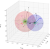 |
Fig. 1. Sketch of principal system components and initial parameters. S and N BHs are represented by large red and blue dashed dots respectively and placed at an initial separation of ΔR. Black holes have initial velocities V1 and V2, for S and N nuclei respectively. Bulges around nuclei have sizes r1 and r2 (each size is equal to 5 Plummer radii of the corresponding bulge), and consist of high-mass particles and low-mass particles, and are represented by purple and green dots respectively. |
Basic N-body models.
The density distribution for each bulge is described as a Plummer sphere (Plummer 1911):
where M*1, 2 is the total stellar mass and R1, 2 is the Plummer radius (Fig. 2). The same central density in each galaxy is provided by scaling the mass, size, and number of particles consistently with BH mass ratio. The fixed Plummer radius for the primary bulge R1 = 200 pc gave us the Plummer radius for the secondary bulge, namely R2 = 160 pc for models A and B, and R2 = 126 pc for models C and D. After the generation of the particle distribution, we simply add the two central SMBHs to the system. Due to the very short dynamical merging scale (a few Myr) of the two bulges, the initial distribution of the particles is quickly mixed up. Separation between the centres of the bulges is 1 kpc according to the observable BH separation.
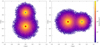 |
Fig. 2. Initial density distributions at projection planes XY and YZ for physical model A. Red and blue dots are S and N BHs respectively. |
To mimic the presence of the molecular gas cloudy and clumpy mass structure in the bulges we introduce a multi-mass prescription to our bulge particle system. Namely, ‘high-mass’ particles (HMPs), which represent perturbers and are associated with giant molecular clouds and/or stellar clusters, and ‘low-mass’ particles (LMPs), which represent field particles and are associated with individual stars. The main set of runs was done using the total number of particles, namely 5 × 10⁵ (except for model B1; see details below), where the number fraction of HMPs is 10% (except for model B4; see details below). At each bulge, the total HMP mass we set equal to the total LMP mass. For the main set of runs (except models B4 and B1; see details below) we use a HMP mass of ∼1.3 × 10⁶ M⊙ and a LMP mass of ∼1.4 × 10⁵ M⊙.
Additionally, to minimize the effect of the initial numerical parameters, we constructed numerical models based on physical model B (Table 1). We use a larger number of particles N = 106 for model B1 (with a HMP mass of ∼6.5 × 10⁵ M⊙ and an LMP mass of ∼7 × 10⁴ M⊙), new randomization for initial particle coordinates and velocities for model B2, a different starting point for PN terms turning on for model B3 (see Sect. 5), and we replace HMP with LMP for model B4 with an LMP mass of ∼2.6 × 10⁵ M⊙.
4. N-body code
For our simulations, we used the publicity available φ-GPU1 code with the blocked hierarchical individual time-step scheme and a 4th, 6th and 8th order Hermite integration schemes of the equation of motions for all particles (Berczik et al. 2011).
In our code we use the generalized “Aarseth” (Makino & Aarseth 1992) type criteria already proposed in the paper Nitadori & Makino (2008):
where
Here, p is the order of the integrator (in this paper p = 4) and a(k) is the kth derivative of acceleration. We moved the accuracy parameter ηp (in this paper η4 = 0.1) out of the fractional power, so that the time step is directly proportional to ηp. The numerator is the same as that for the Aarseth criterion for the fourth-order scheme, and for the denominators we used the terms of the highest orders available. The fractional power is chosen to give the correct dimension of time.
Generally, in a block time-step scheme the individual time steps Δti are replaced by block time-steps Δti, b = (1/2)n, where n satisfies:
In order to minimize computation time, the gravitational forces affecting the particle are divided into two types according to the Ahmad-Cohen scheme. Regular forces acting from neighbour particles and irregular forces acting from more distinct particles, which have different time-steps. This allows us the possibility to calculate irregular forces less often than regular forces.
In the case of close encounters, we should carefully integrate the orbit, and therefore the acceleration of the i particle caused by the j particle with mass mj placed on separation rij in the form:
where ε is the individual softening parameter for each type of particle and α is the reducing factor. In the case of BH, HMP, and LMP, the softening parameters are εBH = 0, εHMP = 10−4, and εLMP = 10−5, respectively. When BHs interact with passing stars, we reduce the softening parameter using the coefficient α = 10−4 for more accurate calculation of acting forces. In other words, for this type of interaction we have effective softening at a level of 7.1 × 10⁻⁷ or 7.1 × 10⁻⁸ respectively for the HMPs and the LMPs, respectively. The individual softening in the code and also the use of the reducing factor for softening allow us to more accurately take into account the dynamical evolution of the BHs even up to the PN merging phase. Our approach is quite similar to the other authors recent N-body PN implementations (see Rantala et al. 2018, 2019; Mannerkoski et al. 2019).
The N-body simulations were run on five clusters: golowood at Kyiv (Ukraine), laohu at Beijing (China), kepler at Heidelberg (Germany), pizdaint at Zurich (Switzerland), and juwels at Jülich (Germany).
5. Post-Newtonian black holes and hardening
As mentioned above, BHs are embedded as special massive relativistic particles located at the centres of bulges. The equation of motion was written via accelerations expressed through positions and velocities in PN formalism. PN theory is an approximate version of general relativity, and therefore in PN terms up to 3.5 PN, the equation of motion can be written schematically in the form

where aPN is the classical Newtonian acceleration. Corrections a1PN, 2PN, 3PN are conservative, i.e., they conserve an appropriate PN form of total energy, while a2.5PN, 3.5PN describe energy losses due to emission of GWs. Acceleration in the center-of-mass frame is
![$$ \begin{aligned} a = \frac{d\mathbf V }{dt}= - \frac{GM}{\Delta R^{2}} [(1+A)\mathbf n +B\mathbf V ], \end{aligned} $$](/articles/aa/full_html/2021/08/aa39859-20/aa39859-20-eq17.gif)
where n is the normalized position vector and V is relative velocity (Blanchet 2006). Coefficients A and B (see Eqs. (182), (183), (185), (186) at Blanchet 2006 and references therein) are the complex functions of masses, velocities, and separations.
Hard binary evolution can be split into two distant regimes: classical and relativistic. Driven by the stellar-dynamical effects, hardening in the classical regime is constant during the long period:
At the next phase, GW emission starts to dominate dissipation force, and hardening drastically decreases. After relativistic and classical hardenings become equal, in the case of only 2.5 PN corrections, average eccentricity and semimajor axis evolution is described as (Peters & Mathews 1963; Peters 1964a,b):
One can obtain the binary hardening during the relativistic regime caused by GW emission (Khan et al. 2012) as
6. Results and discussion
Evolution of SMBHBs happens over three main timescales: the period of time before gravitational binding, the hardening time frame, and the time interval where strong GWs are emitted. The first two phases are described by the classical Newtonian dynamics. During the second phase we have an almost constant N-body hardening rate snb on short timescale. The last time interval is a relativistic mode with combined classical and relativistic hardening rates stot = snb + sgw, where the latter term is dominating. For this reason we take the following strategy for modelling.
As mentioned before, our SMBHB model at an initial separation of 1 kpc is not a bound system. Firstly, we found the binding time of our model binary system in a pure N-body runs and fitted the inverse semimajor axis 1/a with the linear function. The slope of this linear function is our constant N-body hardening. Secondly, we obtained the theoretical relativistic hardening directly from (20). Finally, we compare these hardenings and choose the starting points to turn on the PN terms using two criteria, sgw = 0.3%snb and sgw = 3%snb. In total for models A, B, C, D, B1, and B2 we have one N-body run without PN terms (6 runs total) and two PN runs for each of the Newtonian runs with different starting points tbeg for PN terms (12 runs total) (Table 2). Relativistic sub-runs contain a number that represents the time when we turn on our PN terms. For models B3 and B4 we turn on PN terms directly from tbeg = 0.0. In total, we show 20 individual runs.
Characteristic times for physical and numerical models
Physical and numerical models in the pure N-body regime (Fig. 3) show quick BHs binding from the beginning of the simulations at time t < 10 Myr (Table 2) with a latest binding time tb for model C. Binaries start to be hard at the time th < 12 Myr, with model C taking the longest time because it also has the longest binding time. This time estimation has an error of ±0.66 Myr because of the time interval between the snapshots of the runs. Shrinking of the orbits in the classical regime happens because of the interaction with surrounding stars. The semi-major axis is constantly decreasing as a linear function from gravitational binding almost up to the merging time. The number of particles that interact with the binary drops over time, which is referred to as loss-cone depletion, and the hardening becoming more flat. For our simulations, the PN relativistic terms start to work before this happens. Therefore, in our case, the hardening never stalls. In all of our different physical models, as the primary BH mass increases, we see that the model inverse semimajor axis does not depend on the binary orbital parameters.
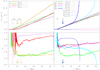 |
Fig. 3. From top to bottom: evolution of inverse semimajor axis and eccentricity in the pure N-body regime for physical models A, B, C, and D (left) and numerical models B1-4 (right) based on physical model B. It is worth noting that for numerical models B3 and B4 we turned on PN terms from the start of simulations. For numerical models, residuals between model B and models B1-4 are shown as colored dashed lines. Colored arrows mark the time when each system becomes bound tb (pale color) and then hard th (intense color). Colors were chosen according to the main color scheme for each model. |
The different numerical models agree well in terms of hardening rate, which shows that hardening rate is independent from the number of particles (in agreement with Berczik et al. 2006; Berentzen et al. 2009), the initial randomization (in agreement with Kompaniiets et al., in prep.), and the starting point of PN terms. For physical models C and D, the eccentricity of binding pairs (0.6–0.9) is higher than for models A and B (0.3–0.4), but this is because the stochastic nature of this process (Wang et al. 2014; Quinlan 1996), as the eccentricity is more or a less random in our N-body simulations. For numerical models with nonphysical differences we see eccentricity at a level of 0.6–0.8. Eccentricity slowly grows with time for both physical and numerical models (Preto et al. 2011).
Evolution with PN terms turned on leads to binaries merging due to GW emission (Fig. A.1, Fig. A.2). We assume that the merging itself happens when the separation between the components is less than 4 Schwarzschild radii, which is equal to 5.2 Mpc for the models with Q = 0.01 and 10.4 Mpc for the models with Q = 0.02. Model D, where the secondary BH has the greatest mass, has the shortest run, and model C, where the primary BH has the lowest mass, has the longest run. The inverse semimajor axis shows a steady increase in the classical regime and a rapid increase at the time when the GW emission is dominant in dissipative force (Fig. A.1, Fig. A.2 left panels). The merging time for physical models ranges from 22 Myr to 53 Myr (Table 2, also see Sobolenko et al. 2016). Eccentricity shows the same merging behavior in classical and relativistic regimes (Fig. A.1, Fig. A.2 right panels): after the binary is formed, the eccentricity is almost constant in a classical regime and approaches zero (circular orbit) in the relativistic regime. Interestingly, in model D, where merging is fastest, the primary BH has the highest mass, and an eccentricity of around 0.9.
Compared to physical model B, model B1, with a different number of particles, and B2, with a different initial randomization of particle positions and velocities, do not show significant differences (also see Kompaniiets et al., in prep.). The choice of starting point tbeg does not affect merging time notably, even for model B3 with PN terms turned on from the beginning. For models B1 and B2, the eccentricity is at a level of 0.6; for model B3 the eccentricity is slightly less, at the level of 0.5–0.6; and for model B4 the eccentricity is higher, at the level of 0.8. The binary of Model B4, with only LMP, merges even more quickly, in ∼30 Myr. The total differences in merging time for all of our numerical models is less then 10% (Table 2). The obtained merging time is greater than that found by Kompaniiets et al. (in prep.); this is due to different initial physical parameters, such as total bulge mass and separation.
For each run, the merging time for both physical and numerical models is not significantly affected by changes in the starting points of the PN terms tbeg. On the other hand, our technique of using two series (with 0.3% and 3% GW hardening compared to the N-body dynamical hardening) for hardening leads to significant computational time savings (Table 3).
Physical computational time at clusters.
To check the effect of choosing the proper starting point we compared modelling and theoretical hardenings for the relativistic regime (Fig. A.3). The relativistic hardening for physical runs of major merging A and B (with mean eccentricity at level of 0.3) shows an earlier decrease than the simple theoretical value. The differences between theoretical and model merging times for model A is 25 Myr and for model B is around 20 Myr. For physical models C and D (with mean eccentricity is > 0.8), the relativistic hardening of the model is of the same order as the theoretical value. For numerical models (with mean eccentricity > 0.5), the difference between the theoretical model values is lower and the best match is observed in models B3 and B4, where we turn on PN terms from the beginning. Numerical models B, B2, and B3 have the same physical parameters, that is, mass of BHs and similar N-body hardening, but they differ in terms of binary eccentricity. According to our restricted number of models, we do not find a dependence of eccentricity on the parameters of our systems, nevertheless it can substantially affect to merging time (Sobolenko et al. 2017). As expected from previous results, the binary can form in a system with any initial eccentricity, and a trend was found from a set of models whereby more circular binaries are formed as cusps become steeper (Khan et al. 2018). Also, Nasim et al. (2020) demonstrated that eccentricity scattering decreases with an increasing number of particles.
7. Conclusions
We present direct N-body modeling with PN corrections up to 3.5 PN for a central SMBHB in the interacting galaxy NGC 6240. Creating a model set with varying physical and numerical parameters allowed us to limit the major merging times for the central binary. In the range of our parameters, we do not find any significant correlation between merging time and BH-to-BH mass or BH-to-bulge mass ratio. We understand that, generally speaking, the set of initial physical conditions can strongly affect of our merging time estimations. Furthermore, mass segregation can strongly affect merging time (see Gualandris & Merritt 2012; Khan et al. 2018), but to discuss this issue in the context of our models with mixed mass prescriptions, further detailed research is needed. Varying numerical parameters (randomization, number of particles, PN starting point) does not strongly affect the merging time for BHs in our models. The estimated time for merging in the galaxy NGC 6240 with the different physical parameters is less than ∼55 Myr. However, this precise value is only valid for our specific combination of initial mass ratios. In the cases presented here, we used a limited range of mass ratios for NGC 6240. Our numerical technique for turning on the relativistic PN forces somewhat after the beginning of the run lead to significant computational time savings. Further detailed research into rare binary and multiple BHs in dense stellar environments (based on observational data) could clarify the dynamical co-evolution of central BHs and their host-galaxies.
Acknowledgments
We acknowledge useful comments and suggestions by our anonymous referee. We were partly supported by the Volkswagen Foundation under the Trilateral Partnerships grant No. 97778. We acknowledge partial support by the Strategic Priority Research Program (Pilot B) Multi-wavelength gravitational wave universe of the Chinese Academy of Sciences (No. XDB23040100). RS acknowledges PKING (PKU-KIAA Innovation NSFC Group, gravitational astrophysics part, NSFC grant 11721303). The work of PB and MS was supported under the special program of the NRF of Ukraine “Leading and Young Scientists Research Support” – “Astrophysical Relativistic Galactic Objects (ARGO): life cycle of active nucleus”, No. 2020.02/0346. MS acknowledges support by the National Academy of Sciences of Ukraine under the Research Laboratory Grant for young scientists No. 0120U100148 and Fellowship of the National Academy of Science of Ukraine for young scientists 2020-2022. PB acknowledges support by the Chinese Academy of Sciences (CAS) through the Silk Road Project at NAOC, the President’s International Fellowship (PIFI) for Visiting Scientists program of CAS and the National Science Foundation of China (NSFC) under grant No. 11673032. The research of PB was also partially funded by the Science Committee of the Ministry of Education and Science of the Republic of Kazakhstan (Grant No. AP08856149). The authors gratefully acknowledge the Gauss Centre for Supercomputing (GSC) e.V. (www.gauss-centre.eu) for funding this project by providing computing time through the John von Neumann Institute for Computing (NIC) on the GCS Supercomputers JURECA and JUWELS at Jülich Supercomputing Centre (JSC).
References
- Begelman, M. C., Blandford, R. D., & Rees, M. J. 1980, Nature, 287, 307 [Google Scholar]
- Bekenstein, J. D. 1973, ApJ, 183, 657 [NASA ADS] [CrossRef] [Google Scholar]
- Berczik, P., Merritt, D., Spurzem, R., & Bischof, H.-P. 2006, ApJ, 642, L21 [NASA ADS] [CrossRef] [Google Scholar]
- Berczik, P., Nitadori, K., Zhong, S., et al. 2011, International conference on High Performance Computing, 8 [Google Scholar]
- Berentzen, I., Preto, M., Berczik, P., Merritt, D., & Spurzem, R. 2009, ApJ, 695, 455 [NASA ADS] [CrossRef] [Google Scholar]
- Beswick, R. J., Pedlar, A., Mundell, C. G., & Gallimore, J. F. 2001, MNRAS, 325, 151 [NASA ADS] [CrossRef] [Google Scholar]
- Blanchet, L. 2006, Liv. Rev. Relativ., 9, 4 [NASA ADS] [CrossRef] [Google Scholar]
- Burke-Spolaor, S. 2011, MNRAS, 410, 2113 [Google Scholar]
- Burke-Spolaor, S., Taylor, S. R., Charisi, M., et al. 2019, A&ARv, 27, 5 [Google Scholar]
- Callegari, S., Mayer, L., Kazantzidis, S., et al. 2009, ApJ, 696, L89 [NASA ADS] [CrossRef] [Google Scholar]
- Callegari, S., Kazantzidis, S., Mayer, L., et al. 2011, ApJ, 729, 85 [NASA ADS] [CrossRef] [Google Scholar]
- Chen, Z., Faber, S. M., Koo, D. C., et al. 2020, ApJ, 897, 102 [Google Scholar]
- Cuadra, J., Armitage, P. J., Alexander, R. D., & Begelman, M. C. 2009, MNRAS, 393, 1423 [Google Scholar]
- eLISA Consortium, (Amaro Seoane, P. et al.) 2013, ArXiv e-prints [arXiv: 1305.5720] [Google Scholar]
- Ellison, S. L., Secrest, N. J., Mendel, J. T., Satyapal, S., & Simard, L. 2017, MNRAS, 470, L49 [NASA ADS] [CrossRef] [Google Scholar]
- Engel, H., Davies, R. I., Genzel, R., et al. 2010, A&A, 524, A56 [NASA ADS] [CrossRef] [EDP Sciences] [Google Scholar]
- Escala, A., Larson, R. B., Coppi, P. S., & Mardones, D. 2005, ApJ, 630, 152 [NASA ADS] [CrossRef] [Google Scholar]
- Fabbiano, G., Wang, J., Elvis, M., & Risaliti, G. 2011, Nature, 477, 431 [NASA ADS] [CrossRef] [Google Scholar]
- Fu, H., Yan, L., Myers, A. D., et al. 2012, ApJ, 745, 67 [Google Scholar]
- Gallimore, J. F., & Beswick, R. 2004, AJ, 127, 239 [NASA ADS] [CrossRef] [Google Scholar]
- Gillessen, S., Plewa, P. M., Eisenhauer, F., et al. 2017, ApJ, 837, 30 [Google Scholar]
- Goicovic, F. G., Sesana, A., Cuadra, J., & Stasyszyn, F. 2017, MNRAS, 472, 514 [Google Scholar]
- Goicovic, F. G., Maureira-Fredes, C., Sesana, A., Amaro-Seoane, P., & Cuadra, J. 2018, MNRAS, 479, 3438 [Google Scholar]
- Green, P. J., Myers, A. D., Barkhouse, W. A., et al. 2011, ApJ, 743, 81 [NASA ADS] [CrossRef] [Google Scholar]
- Gross, A. C., Fu, H., Myers, A. D., Wrobel, J. M., & Djorgovski, S. G. 2019, ApJ, 883, 50 [NASA ADS] [CrossRef] [Google Scholar]
- Gualandris, A., & Merritt, D. 2012, ApJ, 744, 74 [NASA ADS] [CrossRef] [Google Scholar]
- Gualandris, A., Read, J. I., Dehnen, W., & Bortolas, E. 2017, MNRAS, 464, 2301 [Google Scholar]
- Hénon, M. H. 1971, Ap&SS, 14, 151 [NASA ADS] [CrossRef] [Google Scholar]
- Khan, F. M., Preto, M., Berczik, P., et al. 2012, ApJ, 749, 147 [NASA ADS] [CrossRef] [Google Scholar]
- Khan, F. M., Fiacconi, D., Mayer, L., Berczik, P., & Just, A. 2016, ApJ, 828, 73 [NASA ADS] [CrossRef] [Google Scholar]
- Khan, F. M., Berczik, P., & Just, A. 2018, A&A, 615, A71 [EDP Sciences] [Google Scholar]
- Kollatschny, W., Weilbacher, P. M., Ochmann, M. W., et al. 2020, A&A, 633, A79 [EDP Sciences] [Google Scholar]
- Komossa, S., Burwitz, V., Hasinger, G., et al. 2003, ApJ, 582, L15 [NASA ADS] [CrossRef] [Google Scholar]
- Komossa, S., Zhou, H., & Lu, H. 2008, ApJ, 678, L81 [NASA ADS] [CrossRef] [Google Scholar]
- Kormendy, J., & Ho, L. C. 2013, ARA&A, 51, 511 [Google Scholar]
- Kroupa, P., Subr, L., Jerabkova, T., & Wang, L. 2020, MNRAS, 498, 5652 [Google Scholar]
- Lodato, G., Nayakshin, S., King, A. R., & Pringle, J. E. 2009, MNRAS, 398, 1392 [NASA ADS] [CrossRef] [Google Scholar]
- Lousto, C. O., & Healy, J. 2019, Phys. Rev. D, 100 [CrossRef] [Google Scholar]
- Makino, J., & Aarseth, S. J. 1992, PASJ, 44, 141 [NASA ADS] [Google Scholar]
- Maness, H. L., Taylor, G. B., Zavala, R. T., Peck, A. B., & Pollack, L. K. 2004, ApJ, 602, 123 [NASA ADS] [CrossRef] [Google Scholar]
- Mannerkoski, M., Johansson, P. H., Pihajoki, P., Rantala, A., & Naab, T. 2019, ApJ, 887, 35 [Google Scholar]
- Max, C. E., Canalizo, G., & de Vries, W. H. 2007, Science, 316, 1877 [NASA ADS] [CrossRef] [PubMed] [Google Scholar]
- Mayer, L., Kazantzidis, S., Madau, P., et al. 2007, Science, 316, 1874 [NASA ADS] [CrossRef] [PubMed] [Google Scholar]
- McGurk, R. C., Max, C. E., Rosario, D. J., et al. 2011, ApJ, 738, L2 [NASA ADS] [CrossRef] [Google Scholar]
- McGurk, R. C., Max, C. E., Medling, A. M., Shields, G. A., & Comerford, J. M. 2015, ApJ, 811, 14 [Google Scholar]
- Medling, A. M., Ammons, S. M., Max, C. E., et al. 2011, ApJ, 743, 32 [NASA ADS] [CrossRef] [Google Scholar]
- Mezcua, M. 2017, Int. J. Mod. Phys. D, 26, 1730021 [Google Scholar]
- Milosavljević, M., & Merritt, D. 2001, ApJ, 563, 34 [NASA ADS] [CrossRef] [Google Scholar]
- Milosavljević, M., & Merritt, D. 2003, in The Astrophysics of Gravitational Wave Sources, ed. J. M. Centrella, AIP Conf. Ser., 686, 201 [NASA ADS] [CrossRef] [Google Scholar]
- Müller-Sánchez, F., Comerford, J. M., Nevin, R., et al. 2015, ApJ, 813, 103 [Google Scholar]
- Nasim, I., Gualandris, A., Read, J., et al. 2020, MNRAS, 497, 739 [Google Scholar]
- Nitadori, K., & Makino, J. 2008, New Astron., 13, 498 [NASA ADS] [CrossRef] [Google Scholar]
- Paggi, A., Fabbiano, G., Risaliti, G., et al. 2017, ApJ, 841, 44 [CrossRef] [Google Scholar]
- Peres, A. 1962, Phys. Rev., 128, 2471 [CrossRef] [MathSciNet] [Google Scholar]
- Peters, P. C. 1964a, PhD thesis, California Institute of Technology, USA [Google Scholar]
- Peters, P. C. 1964b, Phys. Rev., 136, 1224 [Google Scholar]
- Peters, P. C., & Mathews, J. 1963, Phys. Rev., 131, 435 [NASA ADS] [CrossRef] [Google Scholar]
- Pfeifle, R. W., Satyapal, S., Manzano-King, C., et al. 2019, ApJ, 883, 167 [Google Scholar]
- Planck Collaboration XVI. 2014, A&A, 571, A16 [NASA ADS] [CrossRef] [EDP Sciences] [Google Scholar]
- Plummer, H. C. 1911, MNRAS, 71, 460 [CrossRef] [Google Scholar]
- Preto, M., Berentzen, I., Berczik, P., & Spurzem, R. 2011, ApJ, 732, L26 [NASA ADS] [CrossRef] [Google Scholar]
- Quinlan, G. D. 1996, New Astron., 1, 35 [NASA ADS] [CrossRef] [Google Scholar]
- Rantala, A., Johansson, P. H., Naab, T., Thomas, J., & Frigo, M. 2018, ApJ, 864, 113 [NASA ADS] [CrossRef] [Google Scholar]
- Rantala, A., Johansson, P. H., Naab, T., Thomas, J., & Frigo, M. 2019, ApJ, 872, L17 [NASA ADS] [CrossRef] [Google Scholar]
- Rodriguez, C., Taylor, G. B., Zavala, R. T., et al. 2006, ApJ, 646, 49 [Google Scholar]
- Satyapal, S., Secrest, N. J., Ricci, C., et al. 2017, ApJ, 848, 126 [Google Scholar]
- Sesana, A., Vecchio, A., & Colacino, C. N. 2008, MNRAS, 390, 192 [NASA ADS] [CrossRef] [Google Scholar]
- Sobolenko, M., Berczik, P., & Spurzem, R. 2016, in Star Clusters andBlack Holes in Galaxies across Cosmic Time, eds. Y. Meiron, S. Li, F. K. Liu, & R. Spurzem, 312, 105 [NASA ADS] [Google Scholar]
- Sobolenko, M., Berczik, P., Spurzem, R., & Kupi, G. 2017, Kinematics Phys. Celestial Bodies, 33, 21 [NASA ADS] [Google Scholar]
- Solomon, P. M., Downes, D., Radford, S. J. E., & Barrett, J. W. 1997, ApJ, 478, 144 [Google Scholar]
- Souza Lima, R., Mayer, L., Capelo, P. R., Bortolas, E., & Quinn, T. R. 2020, ApJ, 899, 126 [Google Scholar]
- Tacconi, L. J., Genzel, R., Tecza, M., et al. 1999, ApJ, 524, 732 [NASA ADS] [CrossRef] [Google Scholar]
- Taylor, S., Burke-Spolaor, S., Baker, P. T., et al. 2019, BAAS, 51, 336 [NASA ADS] [Google Scholar]
- Treister, E., Messias, H., Privon, G. C., et al. 2020, ApJ, 890, 149 [NASA ADS] [CrossRef] [Google Scholar]
- Véron-Cetty, M. P., & Véron, P. 2006, A&A, 455, 773 [NASA ADS] [CrossRef] [EDP Sciences] [Google Scholar]
- Vivian, U., Medling, A., Sanders, D., et al. 2013, ApJ, 775, 115 [NASA ADS] [CrossRef] [Google Scholar]
- Wang, L., Berczik, P., Spurzem, R., & Kouwenhoven, M. B. N. 2014, ApJ, 780, 164 [Google Scholar]
- White, S. D. M., & Rees, M. J. 1978, MNRAS, 183, 341 [NASA ADS] [CrossRef] [Google Scholar]
- Woo, J.-H., Cho, H., Husemann, B., et al. 2014, MNRAS, 437, 32 [NASA ADS] [CrossRef] [Google Scholar]
- Yu, Q. 2002, MNRAS, 331, 935 [Google Scholar]
Appendix A: Additional figures
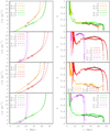 |
Fig. A.1. Inverse semimajor axis (left) and eccentricity (right) evolution for physical models A, B, C, and D composed of N-body and PN runs. The starting point for turning on PN terms from Table 2 is shown with circles. The evolution for the pure N-body regime is cut at the time when the latter PN runs start. |
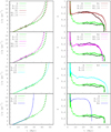 |
Fig. A.2. Inverse semimajor axis (left) and eccentricity (right) evolution for numerical models B1-4 composed of N-body and PN runs. The starting point for turning on the PN terms from Table 2 is shown with circles. The evolution for the pure N-body regime is cut at the time when the latter PN runs start. |
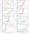 |
Fig. A.3. Hardening comparison for physical models A, B, C, and D (left) and numerical models B1-4 (right) from N-body simulations and theoretical relativistic hardening from (20). |
All Tables
All Figures
|
Fig. 1. Sketch of principal system components and initial parameters. S and N BHs are represented by large red and blue dashed dots respectively and placed at an initial separation of ΔR. Black holes have initial velocities V1 and V2, for S and N nuclei respectively. Bulges around nuclei have sizes r1 and r2 (each size is equal to 5 Plummer radii of the corresponding bulge), and consist of high-mass particles and low-mass particles, and are represented by purple and green dots respectively. |
| In the text | |
|
Fig. 2. Initial density distributions at projection planes XY and YZ for physical model A. Red and blue dots are S and N BHs respectively. |
| In the text | |
|
Fig. 3. From top to bottom: evolution of inverse semimajor axis and eccentricity in the pure N-body regime for physical models A, B, C, and D (left) and numerical models B1-4 (right) based on physical model B. It is worth noting that for numerical models B3 and B4 we turned on PN terms from the start of simulations. For numerical models, residuals between model B and models B1-4 are shown as colored dashed lines. Colored arrows mark the time when each system becomes bound tb (pale color) and then hard th (intense color). Colors were chosen according to the main color scheme for each model. |
| In the text | |
|
Fig. A.1. Inverse semimajor axis (left) and eccentricity (right) evolution for physical models A, B, C, and D composed of N-body and PN runs. The starting point for turning on PN terms from Table 2 is shown with circles. The evolution for the pure N-body regime is cut at the time when the latter PN runs start. |
| In the text | |
|
Fig. A.2. Inverse semimajor axis (left) and eccentricity (right) evolution for numerical models B1-4 composed of N-body and PN runs. The starting point for turning on the PN terms from Table 2 is shown with circles. The evolution for the pure N-body regime is cut at the time when the latter PN runs start. |
| In the text | |
|
Fig. A.3. Hardening comparison for physical models A, B, C, and D (left) and numerical models B1-4 (right) from N-body simulations and theoretical relativistic hardening from (20). |
| In the text | |
Current usage metrics show cumulative count of Article Views (full-text article views including HTML views, PDF and ePub downloads, according to the available data) and Abstracts Views on Vision4Press platform.
Data correspond to usage on the plateform after 2015. The current usage metrics is available 48-96 hours after online publication and is updated daily on week days.
Initial download of the metrics may take a while.