| Issue |
A&A
Volume 651, July 2021
|
|
|---|---|---|
| Article Number | L15 | |
| Number of page(s) | 7 | |
| Section | Letters to the Editor | |
| DOI | https://doi.org/10.1051/0004-6361/202141574 | |
| Published online | 29 July 2021 | |
Letter to the Editor
A tight angular-momentum plane for disc galaxies⋆
1
Kapteyn Astronomical Institute, University of Groningen, Landleven 12, 9747 AD Groningen, The Netherlands
e-mail: This email address is being protected from spambots. You need JavaScript enabled to view it.
2
ASTRON, Netherlands Institute for Radio Astronomy, Oude Hoogeveensedijk 4, 7991 PD Dwingeloo, The Netherlands
3
Observatoire Astronomique de Strasbourg, Université de Strasbourg, 11 rue de l’Université, 67000 Strasbourg, France
4
Space Telescope Science Institute, 3700 San Martin Drive, Baltimore, MD 21218, USA
Received:
16
June
2021
Accepted:
5
July
2021
Abstract
The relations between the specific angular momenta (j) and masses (M) of galaxies are often used as a benchmark in analytic models and hydrodynamical simulations as they are considered to be amongst the most fundamental scaling relations. Using accurate measurements of the stellar (j*), gas (jgas), and baryonic (jbar) specific angular momenta for a large sample of disc galaxies, we report the discovery of tight correlations between j, M, and the cold gas fraction of the interstellar medium (fgas). At fixed fgas, galaxies follow parallel power laws in 2D (j, M) spaces, with gas-rich galaxies having a larger j* and jbar (but a lower jgas) than gas-poor ones. The slopes of the relations have a value around 0.7. These new relations are amongst the tightest known scaling laws for galaxies. In particular, the baryonic relation (jbar − Mbar − fgas), arguably the most fundamental of the three, is followed not only by typical discs but also by galaxies with extreme properties, such as size and gas content, and by galaxies previously claimed to be outliers of the standard 2D j − M relations. The stellar relation (j* − M* − fgas) may be connected to the known j* − M*-bulge fraction relation; however, we argue that the jbar − Mbar − fgas relation can originate from the radial variation in the star formation efficiency in galaxies, although it is not explained by current disc instability models.
Key words: galaxies: kinematics and dynamics / galaxies: spiral / galaxies: dwarf / galaxies: formation / galaxies: evolution / galaxies: fundamental parameters
The associated data catalogue is only available at the CDS via anonymous ftp to cdsarc.u-strasbg.fr (130.79.128.5) or via http://cdsarc.u-strasbg.fr/viz-bin/cat/J/A+A/651/L15
© ESO 2021
1. Introduction
Despite the remarkable diversity of galaxy properties observed in the present-day Universe, a number of physical parameters of galaxies appear to correlate with one another and form tight scaling laws. Such relations are of paramount importance in our quest to understand galaxy formation and evolution (e.g., Tully & Fisher 1977; Fall 1983; Burstein et al. 1997; McGaugh et al. 2000; Marconi & Hunt 2003; Cappellari et al. 2013; Wang et al. 2016).
Since early models of galaxy formation were proposed, it has become clear that mass and angular momentum are two fundamental parameters controlling the evolution of galaxies (e.g., Fall & Efstathiou 1980; Dalcanton et al. 1997; Mo et al. 1998). From an observational point of view, starting from the work by Fall (1983), different authors have characterised the scaling relation between stellar mass (M*) and stellar specific angular momentum (j* = J*/M*, where J* is the angular momentum) as the j* − M* or Fall relation (e.g., Romanowsky & Fall 2012; Obreschkow & Glazebrook 2014; Posti et al. 2018a). This j* − M* law has been widely used in recent years to constrain and test both (semi-)analytic models and hydrodynamical simulations (e.g., Genel et al. 2015; Pedrosa & Tissera 2015; Obreja et al. 2016; Lagos et al. 2017; Tremmel et al. 2017; El-Badry et al. 2018; Stevens et al. 2018; Zoldan et al. 2018; Irodotou et al. 2019).
Mancera Piña et al. (2021, hereafter MP21), derived accurate measurements of the stellar (j*), (cold neutral) gas (jgas), and baryonic (jbar) specific angular momentum for a large sample of irregular spiral and dwarf galaxies (see also e.g., Obreschkow & Glazebrook 2014; Kurapati et al. 2018). They determined the j − M relations for the three components and fitted them with unbroken power laws. They also noticed that the residuals from the best fitting relations correlate with the gas fraction (fgas = Mgas/Mbar, with Mgas and Mbar the gas and baryonic masses, respectively). These trends, also seen in a few semi-analytic models (e.g., Stevens et al. 2018; Zoldan et al. 2018), may indicate that the gas content plays an important role in the j − M relations. In this Letter we build upon that result and report the discovery of new and very tight correlations between mass, specific angular momentum, and gas fraction. We show that disc galaxies across ∼4 orders of magnitude in mass lie in very tight planes in the (j, M, fgas) spaces.
2. Definition of j and galaxy sample
The stellar and gas specific angular momenta of a galaxy are defined as
 (1)
(1)
with R being the galactocentric cylindrical radius, Σi the stellar or gas face-on surface density, and Vi the stellar or gas rotation velocity. Then, j* and jgas can be combined to obtain
 (2)
(2)
For fgas = Mgas/Mbar, we assumed Mbar = M* + Mgas, with Mgas = 1.33MHI, where MHI is the mass of neutral atomic hydrogen and the factor 1.33 accounts for the presence of helium. While we neglected any contribution from molecular gas, in Appendix A we show that its inclusion does not change the results found in this Letter1.
MP21 compiled a high-quality sample of 157 nearby galaxies, predominantly discs. All the galaxies have near-IR photometry and extended HI rotation curves, allowing their stellar discs and rotation velocities to be traced robustly. The sample includes dwarf and massive galaxies, spanning the mass range 7 ≲ log(M*/M⊙) ≲ 11.5, 6 ≲ log(Mgas/M⊙) ≲ 10.5, 8 ≲ log(Mbar/M⊙) ≲ 11.5, and with 0.01 < fgas < 0.97 and a typical relative uncertainty, δfgas/fgas ≈ 0.2 dex (median δfgas ≈ 0.05). While not complete, the sample is representative of the population of regularly rotating nearby discs, like other large samples commonly used in the literature (e.g., Lelli et al. 2016; Ponomareva et al. 2016). Using the near-IR photometry and HI rotation curves, MP21 built cumulative radial profiles for j* (applying a correction to convert Vgas into V*), jgas, and jbar. By selecting only galaxies with radially convergent measurements of angular momentum, they built a sample of 130, 87, and 106 galaxies with accurate j*, jgas, and jbar, respectively. For more details we refer the reader to MP21, and in our associated data catalogues we provide the values of j, M, fgas, distance, and Hubble type for the galaxy sample. These tables are available at the CDS.
MP21 fitted the j − M relations with power laws of the form
![Mathematical equation: $$ \begin{aligned} \log \left(\dfrac{j_i}{\mathrm{kpc\ km\ s}^{-1}} \right) = m_i[\log (M_{i}/M_\odot )-10] + n_i\ , \end{aligned} $$](/articles/aa/full_html/2021/07/aa41574-21/aa41574-21-eq3.gif) (3)
(3)
with the subscript i representing the stellar, gaseous, or baryonic component. The best fitting power laws have slopes mi of about 0.5, 1.0, and 0.6 for stars, gas, and baryons, respectively, and an intrinsic scatter of 0.15 dex.
3. The j − M − fgas planes
3.1. Best fitting planes
MP21 (see their Fig. 7) also found systematic trends with fgas in the residuals of the three j − M laws. To see if introducing a dependence of the j − M laws on fgas can explain these trends, we fitted the (j, M, fgas) data with planes. We fitted the data points with the model
 (4)
(4)
Therefore, we assumed that, in contrast to Eq. (3), ji also depends on fgas2. We performed the fit using the R package HYPER-FIT (Robotham & Obreschkow 2015), including a term for the intrinsic scatter σ⊥. We assumed log-normal uncertainties in j, M, and fgas, and, using a Monte Carlo sampling method, we took into account the fact that uncertainties in the distance, inclination, and mass-to-light ratio of a given galaxy drive correlated uncertainties (also provided in our electronic tables) between log(M), log(j), and log(fgas). We stress that taking these correlations into account is important: Neglecting them can artificially lower the intrinsic scatter of the planes by a factor of two to three.
The best fitting coefficients are reported in Table 1. The orthogonal intrinsic scatter of our best fitting planes is significantly smaller than for the 2D relations. The log-marginal likelihood is also higher (i.e., better) for the 3D planes: by 27, 40, and 43 units for stars, gas, and baryons, respectively. We conclude that the inclusion of fgas into the j − M laws is statistically meaningful.
Coefficients of the best fitting j − M − fgas planes.
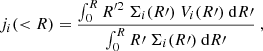
In Fig. 1 we compare the observed distribution of galaxies with our three best fitting planes; the figure shows the 3D j − M − fgas planes projected into the 2D (j, M) spaces. Galaxies are colour-coded according to their fgas, and we overlay our lines of constant fgas derived from our best fitting planes. The fits provide a very good description of the data, in line with the low intrinsic scatter we find for all the planes. By construction, the three j − M − fgas planes are characterised by their M slopes (α*, αgas, and αbar) and fgas slopes (β*, βgas, and βbar). Projected into the (j, M) spaces, the fgas slopes act as a normalisation for j. At fixed M* (Mbar), gas-rich galaxies have a higher j* (jbar) than gas-poor ones, while gas-poor galaxies show a higher jgas. For stars and baryons, the 3D relations become steeper (α* = 0.67 ± 0.03, αbar = 0.73 ± 0.03) than the 2D ones from MP21 (m* = 0.53 ± 0.02, mbar = 0.60 ± 0.02) once fgas is taken into account, while the slope of the gas relation becomes shallower (αgas = 0.78 ± 0.03, mgas = 1.02 ± 0.04). Given the different coefficients, the 2D j − M relations (shown in Fig. 1 as green bands) differ from the projection of the 3D planes in the (j, M) spaces, especially at M < 108 M⊙.
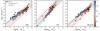 |
Fig. 1. Stellar, gas, and baryonic j − M − fgas planes, projected into the 2D (j, M) spaces. Galaxies are colour-coded according to their fgas and are compared with lines of constant fgas according to Eq. (4) and the best fitting coefficients of Table 1. From red to blue, the lines are at fgas = 0.01, 0.05, 0.2, 0.4, 0.6, 0.8, 1. For comparison, we show in green the best fitting 2D j − M relations from MP21 and their intrinsic scatter. |
A remarkable property of our new scaling laws is their low intrinsic scatter. Given that the baryonic jbar − Mbar − fgas plane incorporates the stellar and cold gas components, we argue that this is likely the most fundamental of the three relations, although its intrinsic scatter is similar to the relation for the gas. Very few other scaling laws are thought to have a comparably low intrinsic scatter, for instance the HI mass-size relation (Wang et al. 2016) or the baryonic Tully-Fisher relation (BTFR; McGaugh et al. 2000; Ponomareva et al. 2017). In fact, our baryonic plane can in principle be used as a distance estimator, with an uncertainty δD/D = (δjbar/jbar)/|2αbar − 1| at fixed Mbar.
3.2. The similarities of the α slopes
The three α slopes of our j − M − fgas planes are relatively close to one another and to the value 2/3 expected for their parent dark matter halos (Fall 1983), which suggests some degree of structural self-similarity between different baryonic components and the dark matter halo. From a mathematical point of view, if we rewrite Eq. (2) in terms of  (with B a function that depends only on fgas) and M* = Mbar(1 − fgas), we obtain
![Mathematical equation: $$ \begin{aligned} j_{\rm bar} = B\ (1-f_{\rm gas})^{\alpha _{*}} \left[\dfrac{j_{\rm gas}}{j_*}f_{\rm gas} + (1-f_{\rm gas}) \right] M_{\rm bar}^{\alpha _{*}}\ . \end{aligned} $$](/articles/aa/full_html/2021/07/aa41574-21/aa41574-21-eq6.gif) (5)
(5)
In a similar way, considering now  (with C a function that depends only on fgas), we find
![Mathematical equation: $$ \begin{aligned} j_{\rm bar} = C\ f_{\rm gas}^{\alpha _{\rm gas}} \left[\dfrac{j_{*}}{j_{\rm gas}}(1-f_{\rm gas}) + f_{\rm gas} \right] M_{\rm bar}^{\alpha _{\rm gas}}\ . \end{aligned} $$](/articles/aa/full_html/2021/07/aa41574-21/aa41574-21-eq8.gif) (6)
(6)
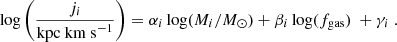
Therefore, at fixed fgas, the slope αbar of the baryonic j − M − fgas plane is expected to be similar to α* and αgas, provided that the ratio jgas/j* is independent of Mbar. As shown in Fig. 2, for our sample, jgas/j*, which is always larger than 1 and mostly within a narrow range (the 16th and 84th percentiles are 1.5 and 3.2, respectively), does not seem to correlate with Mbar, in line with the near-parallelism of the three relations shown in Fig. 1.
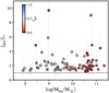 |
Fig. 2. jgas/j* ratio as a function of Mbar. Galaxies are colour-coded by their fgas, and the dashed black line corresponds to jgas/j* = 1. Our galaxies (those with convergent j* and jgas from MP21) cluster at jgas/j* ∼ 2 at all Mbar, albeit with a significant scatter. |
It is worth noticing that the jgas/j* ratio can be related to the relative extent of some characteristic size of the gaseous (Rgas) and stellar (R*) components of galactic discs, given that jgas/j* ≈ RgasVgas/(R*V*) ≈ Rgas/R*. Although this is just an approximation, it can be useful in the physical interpretation of the j − M − fgas relations (e.g., Sect. 4.2.2). In Appendix B we show the expected dependence of jgas/j* on Mbar and fgas derived from our best fitting j* − M* − fgas and jgas − Mgas − fgas planes.
3.3. No outliers of the baryonic j − M − fgas law
In Fig. 3 we plot again our baryonic plane, this time splitting the galaxies into bins of fgas. In each panel we plot lines covering the whole range of fgas within that bin. This allows the tightness of our baryonic relation to be appreciated in more detail.
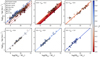 |
Fig. 3. Baryonic jbar − Mbar − fgas plane for our original sample (circles) and a set of extreme galaxies (see text). Top left panel: relation for all the galaxies, while the remaining panels show the galaxies in bins of fgas (given in the top left corner of each panel). First panel, the lines of constant fgas are as in Fig. 1. In the remaining panels, the coloured areas enclose the region delimited by the whole fgas bin. We remark that the coloured lines of our plane are derived by fitting only our data. The rest of the galaxies closely follow our fit. |
We now investigate whether any objects from known galaxy populations could be outliers of our baryonic plane. We do this by comparing our relation – derived using only our sample – with galaxies from the literature that have been argued to be outliers of the 2D j − M relations or that could be outliers given their extreme properties in size, fgas, or rotation velocity.
First, we considered a set of dwarf galaxies from the literature, specifically those from Elson (2017) and Kurapati et al. (2018), that do not overlap with our sample. It was claimed by those authors that some of these galaxies are off the 2D jbar − Mbar relation. We also included the dwarf ‘super thin’ galaxies of Jadhav & Banerjee (2019), which have very high axis ratios and have been suggested to have higher j* than other dwarfs. Next, we looked at the ‘HI extreme galaxies’ (HIXs) of Lutz et al. (2018), which have a particularly high fgas for their M* and are claimed to have higher jbar than average. Moreover, we added a sample of ‘super spiral’ galaxies (di Teodoro et al. 2021), which are very large discs with masses a factor of ten larger than L* galaxies and were also claimed to be outliers of the j* − M* relation (Ogle et al. 2019)3. Finally, we included the ultra-diffuse galaxies (UDGs) AGC 114905 and AGC 242019 (Mancera Piña et al. in prep.; Shi et al. 2021) and the giant low surface brightness galaxies (GLSBs) Malin 1 and NGC 7589 (Lelli et al. 2010). The UDGs are found to be outliers of the BTFR (Mancera Piña et al. 2019, 2020), and both UDGs and GLSBs are extreme galaxies with very extended discs for their M*. With the caveat that some of these galaxies have larger uncertainties than our sample, given the different data quality, we added all these sets of galaxies into the jbar − Mbar − fgas plane in Fig. 3. Remarkably, the location of all of these galaxies, given their fgas, is in very good agreement with the expectation of our scaling relation. We conclude that even extreme galaxies such as HIXs, UDGs, and GLSBs obey the jbar − Mbar − fgas law.
4. Discussion
4.1. Stellar relation: The link with bulge fraction
Previous works (e.g., Fall 1983; Romanowsky & Fall 2012; Cortese et al. 2016; Fall & Romanowsky 2018) found that the relation between j* and M* depends on the bulge-to-total mass fraction, ℬ*. Fall & Romanowsky (2018, hereafter FR18), proposed a model in which discs and spheroids follow relations of the form  but with different normalisation, with spheroids shifting downwards with respect to discs; any given galaxy then has a j* that can be expressed as a linear superposition of a disc and a spheroid (a bulge).
The resemblance of our j* − M* − fgas plane (where at fixed M* a different fgas produces a shift in j*) with the ℬ* relation is clear. Both relations are valid for a variety of morphological types and are preserved along a broad mass span, and with a dependence of j* on M* with a slope of 2/3. The similarities are not unexpected since gas-poor galaxies usually have high ℬ*, though the fgas − ℬ* relation is highly scattered. The above suggests that these two relations may be manifestations of a common physical mechanism. Finally, we note that the scatter is better quantified in the j* − M* − fgas relation with respect to the ℬ* relation given that the uncertainties in ℬ* are difficult to estimate (Salo et al. 2015; FR18).
Interestingly, there is a regime in which the fgas relation makes a different prediction from the ℬ* relation. For galaxies that are almost gas-free and almost bulge-less (we note that galaxies with ℬ* ≲ 0.1−0.2 host pseudo-bulges rather than classical bulges; see Fig. 3 in FR18), the fgas relation expects them to have a lower-than-average j*, while the ℬ* relation predicts a higher-than-average j*. We tested this in Fig. 4 by looking at the four galaxies in our sample with fgas ≤ 0.1 and ℬ* ≤ 0.1 (Salo et al. 2015). We also plot the expected lines given the average ℬ* and fgas for these four galaxies. The points lie close to the fgas relation and deviate from the ℬ* one. However, the evidence is not compelling given the low-number statistics. Finally, it is also important to mention that our galaxy sample is fairly different from that of FR18, with many more gas-dominated discs but a lack of early-type galaxies. These potential differences can be further explored with larger and more complete samples.
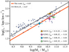 |
Fig. 4. j* − M* relation. Crosses show our galaxies with (fgas, ℬ*) ≤ 0.1. The black and red lines show the expectations from FR18 and this work, respectively. Only a fraction of our range in M* is shown. |
4.2. The origin of the baryonic relation
We then focused our attention on the jbar − Mbar − fgas relation. Its origin is likely related to different galaxy formation processes, such as variations in the angular momentum of the dark matter halos, selective gas accretion within the discs, and different gas accretion histories from the intergalactic medium (Fall 1983; Posti et al. 2018a,b; Stevens et al. 2018; Zoldan et al. 2018). Evolutionary processes such as stellar and active galactic nucleus feedback, mergers, and angular momentum transfer between galaxies and their dark matter halos are arguably also important (Leroy et al. 2008; Dutton & van den Bosch 2012; Romanowsky & Fall 2012; Lagos et al. 2017; Zoldan et al. 2018). Still, while a complex interplay between all these processes is expected, it all results in the tight jbar − Mbar − fgas law we observe. Therefore, it is interesting to check whether or not simple mechanisms are able to capture the dominant processes that give rise to the jbar − Mbar − fgas relation.
4.2.1. Disc instability
We considered two models that have been proposed to explain the jbar − fgas connection as a consequence of gravitational instability. First, Obreschkow et al. (2016) proposed a model that relates fgas with jbar via
 (7)
(7)
with q a stability parameter, σgas the gas velocity dispersion, and G the gravitational constant. Deviations from Eq. (7) may occur depending on the galaxy rotation curve, but they are expected to be small. These results were derived under a number of simplifying assumptions, but less idealised semi-analytic models are found to be in good agreement (Stevens et al. 2018). From Eq. (7), one has log(fgas)∝ 1.12[log(jbar)− log(Mbar)] and jbar ∝ Mbar (this at fixed fgas and assuming a constant σgas). These dependences disagree with our best fitting plane, which has log(fgas)∝2.17log(jbar)−1.59log(Mbar) and  at fixed fgas. Projecting our baryonic plane into the fgas − q diagram shows that galaxies of a given Mbar follow parallel sequences of the form fgas ∝ q1/βbar = q2.22, instead of fgas ∝ q1.124.
Also based on disc instability, Romeo (2020) proposed a set of scaling relations of the form 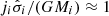 , with i denoting stars or gas and
  a mass-weighted radial average of the velocity dispersion σ. This relation produces the scaling
  (for
(for  , as proposed by Romeo 2020) and jgas ∝ Mgas, very similar to the values found in MP21 for the 2D relations. To incorporate fgas, we rewrote the above expression (using Mi = Mgas = fgasMbar) as
 (8)
(8)
Assuming a constant  , as in Romeo (2020), this relation predicts jgas ∝ Mbar at fixed fgas and jgas ∝ fgas at fixed Mbar. Instead, a corollary of our gas relation is that
  at fixed fgas and that
  at fixed Mbar. Therefore, the relation from Romeo (2020) also seems to depart from our data.
4.2.2. Star formation efficiency
A more general possibility is that the link between jbar, Mbar, and fgas is related to the star formation efficiency in galaxies, as we briefly discuss here. We started by noting that at fixed Mbar the larger the jbar of a galaxy is, the more extended its baryonic distribution will be5. Also, it is well established that gas located in the outskirts of discs forms stars less efficiently than gas closer to the centre (e.g., Leroy et al. 2008). Thus, at fixed Mbar, a galaxy with a large jbar also has a large fgas since a large portion of its mass is located in the less star-forming outer regions. Qualitatively, this is in agreement with the fact that for our entire galaxy sample jgas/j* ≈ Rgas/R* > 1 (see Sect. 3.2). All this suggests that the connection between jbar and fgas may be a reflection of the mechanism responsible for a radially declining star formation efficiency and a radially increasing fgas in galaxy discs (e.g., Leroy et al. 2008; Krumholz et al. 2011; Bacchini et al. 2019), but exploring this idea quantitatively (e.g., by investigating why the jgas/j* ratio is largely independent of Mbar and fgas; see Fig. 2 but also Fig. B.1) is beyond the scope of the present Letter.
5. Conclusions
In this Letter we have used a high-quality sample of disc galaxies to study the relation between their specific angular momenta (j), masses (M), and gas fraction (fgas). The position of our galaxies in the (j, M, fgas) spaces can be described with planes such that galaxies with different fgas follow parallel lines in the projected 2D (j, M) spaces. Remarkably, our planes are preserved along a wide range of mass and morphology with very small (≤0.1 dex) intrinsic scatter, which places the relations amongst the tightest scaling laws for disc galaxies. The jbar − Mbar − fgas plane is arguably the most fundamental, and it is even followed by populations of galaxies with extreme size, mass, and gas content, some of which were previously claimed to be outliers of the 2D j − M relations.
The j* − M* − fgas relation shows analogies with the j* − M* − ℬ* relation (ℬ* being the bulge-to-total mass fraction) previously discussed in the literature. Galaxies with fixed fgas or ℬ* follow parallel relations of the form  . Most galaxies are well described by both the fgas and ℬ* relations, while some discrepancies appear when looking at galaxies with low fgas and low ℬ*.
Finally, we show that models based purely on disc instability do not quantitatively reproduce the observed j − M − fgas relations. We argue that the origin and behaviour of the jbar − Mbar − fgas law is closely related to the spatial distribution of gas and stars within galaxies, as well as to the radial variations in the star formation efficiency.
We stress that our relations offer a unique possibility to quantitatively test a variety of models, including hydrodynamical simulations and semi-analytic models, providing a powerful benchmark for theories on the formation of galactic discs. The slopes and intrinsic scatter of our j − M − fgas planes are important requirements that hydrodynamical simulations and (semi-)analytic models should aim to reproduce.
Our ‘gas’ refers only to the interstellar medium, and there is no attempt to include the largely unconstrained contribution of the gas outside galaxy discs. Although the sum of our gas and stars does not represent the ‘whole’ baryonic budget of a galaxy, we prefer to keep this nomenclature for the sake of consistency with the literature.
Since our planes depend on log(fgas), they become hard to interpret when fgas → 0, preventing us from making extrapolations for galaxies with fgas < 0.01. Using fgas instead of log(fgas) produces less satisfactory fits when compared to the observations, so we prefer log(fgas) despite its limitations when fgas → 0. We also note that, given Eq. (2), the j − M relations cannot all be exactly planes. However, fitting planes in the (j, M, fgas) spaces is a very useful empirical approach.
Since jgas is not available for the super spirals, we assumed jgas = 1.9j*, the median ratio found in the rest of our sample. This has little to no impact given their low gas content (fgas ≈ 0.15).
We note that assuming a non-constant σgas is not enough to alleviate the mentioned discrepancies. To match our relations,  is required; however, it is observed that
  (e.g., Murugeshan et al. 2020).
Second-order effects related to the concentration of the host halo might also be relevant in determining the galaxy sizes (Posti et al. 2020).
Acknowledgments
We would like to thank our referee, Danail Obreschkow, for a very constructive and valuable report, and for his kind assistance regarding the use of HYPER-FIT. We thank Enrico di Teodoro for making available the data on ‘super spiral’ galaxies for us. P.E.M.P., and F.F. are supported by the Netherlands Research School for Astronomy (Nederlandse Onderzoekschool voor Astronomie, NOVA), Project 10.1.5.6. P.E.M.P. benefited from individual comments and discussions with Andrea Afruni and Fernanda Román-Oliveira. L.P. acknowledges support from the Centre National d’Études Spatiales (CNES) and from the European Research Council (ERC) under the European Unions Horizon 2020 research and innovation program (grant agreement No. 834148). G.P. acknowledges support from NOVA, Project 10.1.5.18. E.A.K.A. is supported by the WISE research programme, which is financed by the Netherlands Organization for Scientific Research (NWO). We used SIMBAD and ADS services, as well the Python packages NumPy (Oliphant 2007), Matplotlib (Hunter 2007), and SciPy (Virtanen et al. 2020), for which we are thankful.
References
- Bacchini, C., Fraternali, F., Iorio, G., & Pezzulli, G. 2019, A&A, 622, A64 [NASA ADS] [CrossRef] [EDP Sciences] [Google Scholar]
- Bacchini, C., Fraternali, F., Iorio, G., et al. 2020, A&A, 641, A70 [CrossRef] [EDP Sciences] [Google Scholar]
- Burstein, D., Bender, R., Faber, S., & Nolthenius, R. 1997, AJ, 114, 1365 [NASA ADS] [CrossRef] [Google Scholar]
- Cappellari, M., Scott, N., Alatalo, K., et al. 2013, MNRAS, 432, 1709 [NASA ADS] [CrossRef] [Google Scholar]
- Catinella, B., Saintonge, A., Janowiecki, S., et al. 2018, MNRAS, 476, 875 [NASA ADS] [CrossRef] [Google Scholar]
- Cortese, L., Fogarty, L. M. R., Bekki, K., et al. 2016, MNRAS, 463, 170 [NASA ADS] [CrossRef] [Google Scholar]
- Dalcanton, J. J., Spergel, D. N., & Summers, F. J. 1997, ApJ, 482, 659 [NASA ADS] [CrossRef] [Google Scholar]
- di Teodoro, E. M., Posti, L., & Ogle, P. M. 2021, MNRAS, submitted [Google Scholar]
- Dutton, A. A., & van den Bosch, F. C. 2012, MNRAS, 421, 608 [NASA ADS] [Google Scholar]
- El-Badry, K., Quataert, E., Wetzel, A., et al. 2018, MNRAS, 473, 1930 [NASA ADS] [CrossRef] [Google Scholar]
- Elson, E. C. 2017, MNRAS, 472, 4551 [NASA ADS] [CrossRef] [Google Scholar]
- Fall, S. M. 1983, in Internal Kinematics and Dynamics of Galaxies, ed. E. Athanassoula, IAU Symp., 100, 391 [NASA ADS] [CrossRef] [Google Scholar]
- Fall, S. M., & Efstathiou, G. 1980, MNRAS, 193, 189 [NASA ADS] [CrossRef] [Google Scholar]
- Fall, S. M., & Romanowsky, A. J. 2018, ApJ, 868, 133 [NASA ADS] [CrossRef] [EDP Sciences] [Google Scholar]
- Genel, S., Fall, S. M., Hernquist, L., et al. 2015, ApJ, 804, L40 [NASA ADS] [CrossRef] [Google Scholar]
- Hunter, J. D. 2007, Comput. Sci. Eng., 9, 90 [NASA ADS] [CrossRef] [Google Scholar]
- Irodotou, D., Thomas, P. A., Henriques, B. M., Sargent, M. T., & Hislop, J. M. 2019, MNRAS, 489, 3609 [NASA ADS] [Google Scholar]
- Jadhav, Y. V., & Banerjee, A. 2019, MNRAS, 488, 547 [CrossRef] [Google Scholar]
- Krumholz, M. R., Leroy, A. K., & McKee, C. F. 2011, ApJ, 731, 25 [Google Scholar]
- Kurapati, S., Chengalur, J. N., Pustilnik, S., & Kamphuis, P. 2018, MNRAS, 479, 228 [NASA ADS] [CrossRef] [Google Scholar]
- Lagos, C. d. P., Theuns, T., Stevens, A. R. H., et al. 2017, MNRAS, 464, 3850 [NASA ADS] [CrossRef] [Google Scholar]
- Lelli, F., Fraternali, F., & Sancisi, R. 2010, A&A, 516, A11 [NASA ADS] [CrossRef] [EDP Sciences] [Google Scholar]
- Lelli, F., McGaugh, S. S., & Schombert, J. M. 2016, AJ, 152, 157 [Google Scholar]
- Leroy, A. K., Walter, F., Brinks, E., et al. 2008, AJ, 136, 2782 [Google Scholar]
- Lutz, K. A., Kilborn, V. A., Koribalski, B. S., et al. 2018, MNRAS, 476, 3744 [NASA ADS] [CrossRef] [Google Scholar]
- Mancera Piña, P. E., Fraternali, F., Adams, E. A. K., et al. 2019, ApJ, 883, L33 [CrossRef] [Google Scholar]
- Mancera Piña, P. E., Fraternali, F., Oman, K. A., et al. 2020, MNRAS, 495, 3636 [CrossRef] [Google Scholar]
- Mancera Piña, P. E., Posti, L., Fraternali, F., Adams, E. A. K., & Oosterloo, T. 2021, A&A, 647, A76 [CrossRef] [EDP Sciences] [Google Scholar]
- Marconi, A., & Hunt, L. K. 2003, ApJ, 589, L21 [Google Scholar]
- McGaugh, S. S., Schombert, J. M., Bothun, G. D., & de Blok, W. J. G. 2000, ApJ, 533, L99 [NASA ADS] [CrossRef] [PubMed] [Google Scholar]
- Mo, H. J., Mao, S., & White, S. D. M. 1998, MNRAS, 295, 319 [Google Scholar]
- Murugeshan, C., Kilborn, V., Jarrett, T., et al. 2020, MNRAS, 496, 2516 [NASA ADS] [CrossRef] [Google Scholar]
- Obreja, A., Stinson, G. S., Dutton, A. A., et al. 2016, MNRAS, 459, 467 [NASA ADS] [CrossRef] [Google Scholar]
- Obreschkow, D., & Glazebrook, K. 2014, ApJ, 784, 26 [NASA ADS] [CrossRef] [Google Scholar]
- Obreschkow, D., Glazebrook, K., Kilborn, V., & Lutz, K. 2016, ApJ, 824, L26 [CrossRef] [Google Scholar]
- Ogle, P. M., Jarrett, T., Lanz, L., et al. 2019, ApJ, 884, L11 [Google Scholar]
- Oliphant, T. E. 2007, Comput. Sci. Eng., 9, 10 [Google Scholar]
- Pedrosa, S. E., & Tissera, P. B. 2015, A&A, 584, A43 [NASA ADS] [CrossRef] [EDP Sciences] [Google Scholar]
- Ponomareva, A. A., Verheijen, M. A. W., & Bosma, A. 2016, MNRAS, 463, 4052 [NASA ADS] [CrossRef] [Google Scholar]
- Ponomareva, A. A., Verheijen, M. A. W., Peletier, R. F., & Bosma, A. 2017, MNRAS, 469, 2387 [NASA ADS] [CrossRef] [Google Scholar]
- Posti, L., Fraternali, F., Di Teodoro, E. M., & Pezzulli, G. 2018a, A&A, 612, L6 [NASA ADS] [CrossRef] [EDP Sciences] [Google Scholar]
- Posti, L., Pezzulli, G., Fraternali, F., & Di Teodoro, E. M. 2018b, MNRAS, 475, 232 [NASA ADS] [CrossRef] [Google Scholar]
- Posti, L., Famaey, B., Pezzulli, G., et al. 2020, A&A, 644, A76 [CrossRef] [EDP Sciences] [Google Scholar]
- Robotham, A. S. G., & Obreschkow, D. 2015, PASA, 32, e033 [NASA ADS] [CrossRef] [Google Scholar]
- Romanowsky, A. J., & Fall, S. M. 2012, ApJS, 203, 17 [Google Scholar]
- Romeo, A. B. 2020, MNRAS, 491, 4843 [NASA ADS] [CrossRef] [Google Scholar]
- Salo, H., Laurikainen, E., Laine, J., et al. 2015, ApJS, 219, 4 [NASA ADS] [CrossRef] [Google Scholar]
- Shi, Y., Zhang, Z.-Y., Wang, J., et al. 2021, ApJ, 909, 20 [CrossRef] [Google Scholar]
- Stevens, A. R. H., Lagos, C. d. P., Obreschkow, D., & Sinha, M. 2018, MNRAS, 481, 5543 [CrossRef] [Google Scholar]
- Tremmel, M., Karcher, M., Governato, F., et al. 2017, MNRAS, 470, 1121 [CrossRef] [Google Scholar]
- Tully, R. B., & Fisher, J. R. 1977, A&A, 500, 105 [Google Scholar]
- Virtanen, P., Gommers, R., Oliphant, T. E., et al. 2020, Nat. Methods, 17, 261 [Google Scholar]
- Wang, J., Koribalski, B. S., Serra, P., et al. 2016, MNRAS, 460, 2143 [Google Scholar]
- Zoldan, A., De Lucia, G., Xie, L., Fontanot, F., & Hirschmann, M. 2018, MNRAS, 481, 1376 [NASA ADS] [CrossRef] [Google Scholar]
Appendix A: The role of molecular gas
In this Letter we have assumed Mgas = 1.33MHI and jgas = jHI, neglecting any contribution from molecular (H2) and ionised gas. Here we show that observationally motivated corrections to account for the presence of H2 do not change our results.
To account for MH2 in our estimates of Mgas, we relied on the results from Catinella et al. (2018), who provide measurements of the ratio MH2/MHI as a function of M* for a large sample of nearby galaxies. We fitted a linear relation to their binned measurements (see their Fig. 9 and Table 3), finding
 (A.1)
(A.1)
The scatter is large, and we adopted an uncertainty of 50% in MH2. With this, we redefined Mgas = 1.33(MHI + MH2) and updated Mbar and fgas accordingly. For massive discs, the correction to Mgas is about 0.1 dex, which is smaller than the typical uncertainty in Mgas (∼0.13 dex); the correction is even smaller for the dwarfs. The change in fgas is of the same order, also being negligible at low masses and changing by up to 0.1 dex at the high-mass end; this change is also of the order of the typical uncertainty in fgas. Correspondingly, Mbar remains largely unchanged since the correction is smaller than 0.04 dex at all masses.
Including H2 can also affect jgas, as seen from the equation
 (A.2)
(A.2)
where jHI and jH2 are the specific angular momenta of the atomic and molecular gas components, respectively, and fatm is the atomic-to-total gas ratio, fatm = MHI/(MHI + MH2).
Obreschkow & Glazebrook (2014) provide measurements of jHI, jH2, and jgas for a sample of 16 spiral galaxies. In addition to this, we computed jHI for four galaxies in our sample that have surface densities and CO rotation curves available from Bacchini et al. (2020). The typical ratio between jgas and jHI is 0.85, which translates into a shift of 0.07 dex. Thus, on average, including H2 implies a correction to jHI such that log(jgas) = log(jHI)−0.07. The correction is of the same order as the average uncertainty in jgas, 0.08 dex.
We again fitted the 3D relations taking into account the above corrections to Mgas, fgas, jgas, and Mbar. The new coefficients for stars, gas, and baryons are listed in Table A.1. As expected, they are fully consistent with those reported in Table 1 within the uncertainties. Therefore, we conclude that including H2 does not have a significant effect on the derivation of the j − M − fgas laws, and our results remain unchanged.
Same as Table 1 but taking into account the presence of molecular gas.
Appendix B: The jgas/j* ratio from our best fitting planes
The jgas/j* ratio can be obtained directly from our individual galaxy measurements, as shown in Fig. 2. Nevertheless, jgas/j* can also be obtained by using our best fitting stellar and gas relations. This allows us to extrapolate jgas/j* to values of fgas and Mbar beyond our observations and, in principle, to neglect the observational uncertainties since they are accounted for in our best fitting planes. Using Eq. (4) the ratio becomes
![Mathematical equation: $$ \begin{aligned} \log (j_{\rm gas}/j_*)&= \alpha _{\rm gas}\log (f_{\rm gas} M_{\rm bar}) - \alpha _{*}\log [(1-f_{\rm gas}) M_{\rm bar}] \nonumber \\&\quad + (\beta _{\rm gas}-\beta _{*})\log (f_{\rm gas}) + \gamma _{\rm gas}-\gamma _{*}\ , \end{aligned} $$](/articles/aa/full_html/2021/07/aa41574-21/aa41574-21-eq25.gif) (B.1)
(B.1)
and the corresponding surface according to Table 1 is shown in Fig. B.1. As can be seen, most of our galaxies lie within a region where jgas/j* ∼ 2. It will be interesting to see where other large samples of galaxies would lie in Fig. B.1 and whether they also follow the expected dependence of jgas/j* on Mbar and fgas.
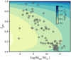 |
Fig. B.1. Relation between Mbar, fgas, and the best fitting jgas/j* ratio according to Eq. (B.1). The background shows increasing levels of jgas/j*, and the grey points show our galaxies with convergent measurements of jgas and j*. |
All Tables
All Figures
|
Fig. 1. Stellar, gas, and baryonic j − M − fgas planes, projected into the 2D (j, M) spaces. Galaxies are colour-coded according to their fgas and are compared with lines of constant fgas according to Eq. (4) and the best fitting coefficients of Table 1. From red to blue, the lines are at fgas = 0.01, 0.05, 0.2, 0.4, 0.6, 0.8, 1. For comparison, we show in green the best fitting 2D j − M relations from MP21 and their intrinsic scatter. |
| In the text | |
|
Fig. 2. jgas/j* ratio as a function of Mbar. Galaxies are colour-coded by their fgas, and the dashed black line corresponds to jgas/j* = 1. Our galaxies (those with convergent j* and jgas from MP21) cluster at jgas/j* ∼ 2 at all Mbar, albeit with a significant scatter. |
| In the text | |
|
Fig. 3. Baryonic jbar − Mbar − fgas plane for our original sample (circles) and a set of extreme galaxies (see text). Top left panel: relation for all the galaxies, while the remaining panels show the galaxies in bins of fgas (given in the top left corner of each panel). First panel, the lines of constant fgas are as in Fig. 1. In the remaining panels, the coloured areas enclose the region delimited by the whole fgas bin. We remark that the coloured lines of our plane are derived by fitting only our data. The rest of the galaxies closely follow our fit. |
| In the text | |
|
Fig. 4. j* − M* relation. Crosses show our galaxies with (fgas, ℬ*) ≤ 0.1. The black and red lines show the expectations from FR18 and this work, respectively. Only a fraction of our range in M* is shown. |
| In the text | |
|
Fig. B.1. Relation between Mbar, fgas, and the best fitting jgas/j* ratio according to Eq. (B.1). The background shows increasing levels of jgas/j*, and the grey points show our galaxies with convergent measurements of jgas and j*. |
| In the text | |
Current usage metrics show cumulative count of Article Views (full-text article views including HTML views, PDF and ePub downloads, according to the available data) and Abstracts Views on Vision4Press platform.
Data correspond to usage on the plateform after 2015. The current usage metrics is available 48-96 hours after online publication and is updated daily on week days.
Initial download of the metrics may take a while.