| Issue |
A&A
Volume 651, July 2021
|
|
|---|---|---|
| Article Number | A28 | |
| Number of page(s) | 6 | |
| Section | Stellar structure and evolution | |
| DOI | https://doi.org/10.1051/0004-6361/202140629 | |
| Published online | 06 July 2021 | |
Empirically revealed properties of Rieger-type cycles of stellar activity
1
Space Research Institute, Austrian Academy of Sciences, Schmiedlstrasse 6, 8042 Graz, Austria
e-mail: This email address is being protected from spambots. You need JavaScript enabled to view it.
2
Institute of Astronomy of the Russian Academy of Sciences, 119017 Moscow, Russia
3
Institute of Laser Physics, SB RAS, Novosibirsk 630090, Russia
Received:
22
February
2021
Accepted:
14
April
2021
Abstract
Context. The Rieger cycles were discovered in the Sun as a specific 154-day periodicity of flare occurrence; they strongly influence terrestrial space weather. This phenomenon is far from being understood. Various proposed mechanisms for this periodicity need further verification in stars with stellar parameters different from those of the Sun.
Aims. In this work, we study the Rieger-type cycle (RTC) periods PRTC of stellar activity surveyed in the photometric data of the Kepler space telescope.
Methods. The processing of 1726 stellar light curves reveals statistics of PRTC values for different main-sequence stars with different effective temperatures Teff and periods of rotation P. This study uses as an index of stellar activity the squared amplitude of the first rotational harmonic A12 of the stellar light curve variability.
Results. The obtained information on PRTC of the considered stars confirms the phenomenological analogy between stellar RTCs and the solar Rieger cycles. Two types of RTCs were found: (1) activity cycles with PRTC independent on the stellar rotation, which are typical for the stars with Teff ≲ 5500 K, and (2) activity cycles with PRTC proportional to the stellar rotation period P, which take place on stars with Teff ≳ 6300 K. These two types of RTCs can be driven by the Kelvin and Rossby waves, respectively. The Rossby wave-driven RTCs show a relation with the location of tachocline at shallow depths in the hot stars. This confirms the theoretical predictions of the connection of the RTC with the tachocline. At the same time, the Kelvin wave-driven RTCs do not show this connection. Apparently, both types of wave drivers of RTCs can coexist, resulting in the joint modulation of the magnetic flux tubes emergence by Kelvin and Rossby waves, and the corresponding behavior of PRTC.
Conclusions. The signatures of two types of wave drivers discovered for RTCs and their different relations with the tachocline call for a revision and further elaboration of the theory of RTCs.
Key words: stars: activity / stars: rotation / stars: statistics / techniques: photometric / surveys / waves
© ESO 2021
1. Introduction
The Rieger cycles were discovered in the Sun as a specific 154-day periodicity of flare occurrence (Rieger et al. 1984). Later on the Rieger-type cycles (RTCs), with periods PRTC from 109 to 276 days, were confirmed in the solar magnetic field and sunspot indexes (e.g., Feng et al. 2017; Gurgenashvili et al. 2016 and references therein). The corresponding periodicity has been also revealed in auroral datasets (Silverman 1990), geomagnetic activity (Singh 2017), the atmospheric electric potential gradient, and the neutron count rate (Silva & Lopes 2017), and even in a nuclear decay rate (Sturrock et al. 2011). Hence, the RTCs are an important factor with a significant environmental impact. They also influence the space weather conditions crucial for space missions.
At the same time, the nature of RTCs is still not understood. Since this phenomenon is more pronounced during the activity maxima (Zaqarashvili et al. 2010), we can suppose that the Rieger-type periodicity relates with modulation of the magnetic dynamo process. Zaqarashvili et al. (2010) consider several potential explanations involving the inertial g- and r-waves (Rossby waves), which are supposed to modulate the magnetic flux emersion. In general, there are many wave modes in the rotating plasma (Lou 2000), especially in the presence of a magnetic field (Zaqarashvili 2018). Various modes of Rossby waves are commonly suggested as a cause of RTCs (e.g., Lou 2000; Gurgenashvili et al. 2016; Zaqarashvili 2018; Raphaldini et al. 2019). At the same time, the validity of the mechanisms proposed in the above-cited papers for the solar RTCs needs further verification as related to the stars with parameters different from those of the Sun.
The dispersion equations (e.g., Lou 2000; Zaqarashvili 2018) of Rossby waves in solar interiors predict the proportionality of short (as compared to the primary long cycle) periods of stellar activity Pcyc to the stellar rotation period P. However, an empiric study of 32 young solar-type stars with the short-period secondary cycles 55 ≤ Pcyc ≤ 1428 days (Distefano et al. 2017) revealed independence of Pcyc on P. This contradiction could be due to an interference of different physical drivers of the short-period stellar activity cycles. Such P-independent cycles like those with Pcyc ∼ 480 days (≈1.3 yr) are observed in the solar spot and magnetic data (Feng et al. 2017), and in the activity of some other stars (Vida et al. 2014; Kitze et al. 2017). For the Sun the ∼480-day activity cycles were attributed with Kelvin magneto-waves (Gachechiladze et al. 2019), which yield no proportionality between Pcyc and P (see Eqs. (15) and (18) in Gachechiladze et al. 2019). Hence, in view of the possibility of different mechanisms for short-period cycles, they deserve special attention, in particular with respect to RTCs on different kinds of stars.
In this paper we present the results of a survey of the short-period secondary cycles of stellar activity based on the approaches elaborated in our previous studies (Arkhypov et al. 2015a,b, 2016, 2018a,b,c). The method is explained in Sect. 2; the obtained results are described in Sect. 3; and we present our conclusions in Sect. 4.
2. Survey of short-period stellar activity
The methodology of our survey has several important differences from analogous studies undertaken previously by other researchers. Traditionally, the long-period primary cycles of stellar activity (Pcyc ≳ 103 days) were considered and investigated because of their maximum spectral power (e.g., Reinhold et al. 2017; Boro Saikia et al. 2018; Olspert et al. 2018; Bondar’ et al. 2020 and references therein). Sometimes the shorter secondary oscillations of activity (Pcyc < 103 days) were also studied, but without differentiation (e.g., Distefano et al. 2017; Reinhold et al. 2017). Among the shorter cycles there are different kinds of periodicity: (a) RTCs (Massi et al. 2005), (b) analogs of the solar spot cycle with Pcyc ≈ 1.3 yr, and (c) short-period magnetic activity oscillations (Jeffers et al. 2018). The traditional spectral analysis, based on the simple Fourier transform, focuses on the most powerful long-period stellar activity cycles. Therefore, to study the usually non-dominating short-period RTCs we used a modified analysis approach that is especially sensitive to this type of periodicity. In addition, we considered in our survey the stars with the most probable presence of RTCs.
2.1. Compilation of dataset
According to the current hypotheses (Zaqarashvili et al. 2010; Zaqarashvili 2018; Gurgenashvili et al. 2016; Raphaldini et al. 2019), the RTCs are related with tachocline at the border between the stellar radiative region and convective zone. The tachocline is a common attribute of the Sun and solar-type stars. Therefore, our survey was addressed to the main-sequence (MS) stars with well-developed convective zones. Sub-giants were considered as well, as they also possess convective zones and radiative regions, whereas the giant stars were excluded because of their pulsations.
As a preliminary set for the analysis, we take the light curves of about two thousand stars without exoplanetary transits from the data archive of the space telescope Kepler. This set was also considered in our previous studies in Arkhypov et al. (2015a,b, 2016, 2018a,b,c). The Kepler mission gives the highest quality stellar photometry data series, which were already analyzed in our pilot study of short-period cycles of stellar activity in Arkhypov et al. (2015b). These objects were selected with the account of the estimated surface gravity log(g[cm s−2]) ≥ 4.0 typical for MS stars. However, the most recent version of the Kepler stellar catalog in the Mikulski Archive for Space Telescopes (MAST)1 reclassifies some of the previously selected stars in our set as sub-giants and even giants. Therefore, we excluded from the previously considered stellar set the objects with low surface gravity log(g[cm s−2]) < 4.2, according to the newest data in MAST. As a result, we deal here with the remaining selected 1726 MS objects. Their distribution in the (log(g),Teff) − plane, an analog of the HR diagram, is shown in Fig. 1.
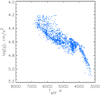 |
Fig. 1. Distribution of the analyzed stellar set in the (log(g),Teff)-plane, i.e., an analog of the HR diagram. The values of the stellar surface gravity log(g) and effective temperature Teff are from the newest version of Kepler Archive DR25 (MAST). |
The stellar rotation periods P, needed for our study, are extracted from the catalog by McQuillan et al. (2014). They were determined using the modulation of Kepler stellar light curves caused by the starspots. To avoid problems that arise from stellar pulsations and insufficient count number per stellar rotation (in case of short periods P < 0.5 days), and from poor rotation statistics (for long periods P > 30 days), we considered only stars with 0.5 ≤ P ≤ 30 days.
2.2. Characterizing short-period activity cycles
To estimate the value of Pcyc we analyzed the rotational modulation of stellar photometry flux F, which reflects the longitudinal distribution of starspots. The stellar light curves from the Kepler mission archive (PDCSAP_FLUX)2 that we used for this purpose were already preprocessed to correct for instrumental and environmental effects. As in our previous studies Arkhypov et al. (2015a,b, 2016, 2018a,b,c), we consider here a normalized amplitude A1 of the first rotational harmonic of the light curve (i.e., the Fourier-harmonic with period P). In Arkhypov et al. (2016), taking the Sun as an example of star, it was shown that the squared amplitude of this value,  , is statistically proportional to the starspot number, and therefore it can be used as a kind of stellar activity index. The activity index
  , in contrast with traditional indexes based on variance of the light curve, is practically insensitive to the photon noise. It also minimally depends on the residual (after flare removal) short-time phenomena, such as short-periodic pulsations and eruptive brightenings. Moreover, the index
  was shown to be more sensitive to the short-period cycles of solar activity than the sunspot number (see, e.g., Fig. 3 in Arkhypov et al. 2016). The technical details of its calculation can be found in Arkhypov et al. (2015a,b, 2018c). Figure 2 shows the time series of index
  , demonstrating the short-period Rieger cycles of activity with a typical duration of 100 to 200 days on the Sun (panel A), as well as their analogs (i.e., RTCs) in some yellow dwarfs in panels B and C. As can be seen in this figure, the RTCs look like stochastically modulated oscillations of the activity.
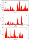 |
Fig. 2. Examples of RTC modulations in time series of activity index |

In Arkhypov et al. (2015b) we elaborated two methods for the estimation of the duration of short-period stellar activity cycles. They were successfully applied to the fast rotating stars, with periods 1 < P < 4 days. However, these methods become less efficient in the case of slow stellar rotation (P ≳ 10 days) because the decreasing statistics of the rotations and the increasing lags of the autocorrelation analysis restrict the method’s applicability. Hence, instead of the previously used methods, for the analysis of activity cycles in the considered stellar sample we applied the standard Fourier transform, which in spite of the above-mentioned limitations was demonstrated in Arkhypov et al. (2015b) to be a possible way to study Pcyc. Figure 3 shows an example of clear oscillations of the activity level in the stars KIC 7671028, KIC 8144578, and KIC 12365719. The occasional gaps in series of activity index  were filled using linear interpolation. After applying the Fourier transform to these data, the resulting power spectra (i.e., the distribution of squared amplitudes of Fourier spectral harmonics over the periods PF) were obtained (Figs. 3B, D, F). As can be seen, all these spectra have the signatures of increasing power in the long-period domain, and also have very pronounced peaks in the range 20 < PF < 200 days. The corresponding periods PF = Ppeak of such spectral peaks with the maximum amplitude for PF < 103 days are considered to be the estimates of the periods of the short cycles of activity of the considered stars, i.e., Pcyc ≡ Ppeak.
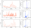 |
Fig. 3. Oscillatory behavior of the activity index |

Figure 4 shows the distribution of the log of the estimates of Ppeak (blue squares) versus the log of the stellar rotation periods P for solar-type stars with 5500 < Teff < 6000 K. We can see that these estimates are clustered in a cloud with the dominating presence of long-periodic activity cycles in the considered stars. At the same time, some of the stars in the analyzed sample demonstrate the domination of short-periodic cycles which form the pronounced lower border of the cluster in the diagram in Fig. 4. The solar RTCs indicated for comparison (orange circle with a range bar) are also located at the lower border, in the region of the shortest periods of the cluster. This gives the reason to consider the RTCs as the shortest component of activity cycles. Hence, we can study the behavior of PRTC versus P, or another parameter (e.g., Teff), by tracing the lower border of the log(Ppeak) cluster.
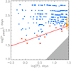 |
Fig. 4. Distribution of the log(Ppeak) estimates vs. log of the stellar rotation periods P for the solar-type stars with 5500 < Teff < 6000 K. For comparison, the position of solar RTCs is indicated with a yellow circle which corresponds to Ppeak = 154 days according to Rieger et al. (1984). The bar denotes the total range of solar RTCs according to Feng et al. (2017). The red line shows the linear regression of the lower border set of the log(Ppeak) cluster, obtained for the minimum values of Ppeak (red crossed squares) defined for the sequential ten intervals of P. The gray area in the lower right corner of the plot indicates the detection limit zone for Ppeak, restricted by the Nyquist frequency (2P)−1. |
For this purpose, in Fig. 4 we divided the whole region of the logarithm of rotation periods 0.5 < P < 30 days of the considered sample of the solar-type stars into ten sequential bins, and found the minimum values of log(Ppeak) in each bin (shown as red crossed squares in Fig. 4). The lower border value set of the log(Ppeak) cluster obtained in this way was approximated as
 (1)
(1)
where D = 0.34 ± 0.09 and C = 1.64 ± 0.07 are the constants fitted by the least-squares method. We note that the solar RTCs (yellow circle with a range bar in Fig. 4) nicely fit the obtained regression. This confirms the background idea of the proposed approach, that the lower border of the log(Ppeak) cluster reproduces the behavior of  .
.
To look at this idea from another perspective and to verify our approach, we constructed a diagram of log(Ppeak) estimates versus log(Teff), which is shown in Fig. 5, for a subset of fast rotating stars with periods 1 < P < 4 days. This subset was analyzed in Arkhypov et al. (2015b) on the basis of the same activity index  , but using methods different from the direct Fourier transform for the estimation of the short-period activity cycle duration. At the same time, to obtain the Ppeak values for the diagram in Fig. 5, we still applied the Fourier transform. Then, following an approach similar to that applied for the analysis of the diagram in Fig. 4, and keeping in mind that RTCs are the shortest detected cycles, we identified the lower border set of the log(Ppeak) cluster in Fig. 5 (i.e., the set of minimum values of Ppeak) and approximate it with a linear regression. After that we compared the outcome of this approach with the linear regression of log(Pcyc(log(Teff))) obtained in Arkhypov et al. (2015b).
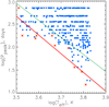 |
Fig. 5. Distribution of the log(Ppeak) estimates vs. log(Teff) for the same subset of fast rotating stars with 1 < P < 4 days as processed by other methods in Arkhypov et al. (2015b). The red line shows the linear regression of the lower border set of the log(Ppeak) cluster, obtained for the minimum values of Ppeak (red crossed squares) defined for the sequential ten intervals of Teff. The green line shows linear regression of log(Pcyc(log(Teff))) obtained in Arkhypov et al. (2015b) by other methods. The detection limit zone for Ppeak, restricted by the Nyquist frequency (2P)−1 for the considered subset of fast rotators appears outside of the displayed frame. |
As can be seen in Fig. 5, the lower border linear regression of the log(Ppeak) cluster (red line) has practically the same inclination  as the inclination −3.70 ± 0.12 of the log(Pcyc(log(Teff))) regression (green line) in Arkhypov et al. (2015b). The difference between these two approximations is quite an insignificant value: ∼0.35 dex equivalent to 1.6σ, where
  is a standard error. The whole range of differences between the values, predicted by both regressions, from 0.3 to 0.4 dex, corresponds to the typical dispersion of estimates of log(Pcyc) in Fig. 15 in Arkhypov et al. (2015b). Therefore, the method proposed here, based on the approximation of the lower border of the log(Ppeak) cluster, allows us to measure the power indexes D and
  in the functional dependencies PRTC(P) ∝ PD and
  , and thus it can be used for the diagnostics of RTCs.
3. Phenomenology and diagnostics of RTCs
The diagrams in Fig. 6 are prepared in the same way as that used to create the diagram in Fig. 4. But they are made for the subsets of cold stars, with 3000 < Teff < 4000 K (Fig. 6A), and hot stars, with 6300 < Teff < 7000 K (Fig. 6B) separately, extracted from the whole analyzed stellar sample. According to Fig. 6A, the lower border of the log(Ppeak) cluster, which reflects the behavior of PRTC(P) ∝ PD, shows a very weak dependence on P, resulting in a negligible power index D = −0.07 ± 0.07. This excludes the mechanism of Rossby waves as a driver of RTCs for the considered subset of cold stars, which would predict the proportionality PRTC ∝ P (i.e., D = 1). Such proportionality is seen in the behavior of the lower border of log(Ppeak) cluster in Fig. 6B, obtained for the subset of hot stars. Its linear regression (Eq. (1)), calculated using the same number of bins (10) as in the case in Fig. 4, yields the close to unity power index D = 0.85 ± 0.09. Based on this, we can conclude for the first time about the domination of Rossby waves as a driver of short-period activity cycles on such hot stars.
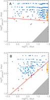 |
Fig. 6. Same as the Fig. 4 diagrams of log(Ppeak) distribution vs. log(P), but for cold (panel A) and hot (panel B) stars with 3000 < Teff < 4000 K and 6300 < Teff < 7000 K, respectively. |
In order to check the potential effect of the number of bins on the selection of the lower border set within the log(Ppeak) cluster in Fig. 6B and the definition of its linear regression coefficients, we tried this procedure for 5, 10, 15, and 20 bins. As a result, all the obtained values of the power index D appeared to be around unity, within the ranges of their corresponding definition errors. However, for 15 and 20 bins the definition errors were more than two times higher than those for 5 and 10 bins. At the same time, considering only 5 bins yields only 5 points for the regression. Altogether, using 10 bins through the whole analysis reported here seems to be an optimal compromise between the number of points, which approximate the lower border of the log(Ppeak) cluster, and the definition accuracy for the power index D in the dependence PRTC(P) ∝ PD.
Figure 7A presents the change in the power index D depending on the stellar effective temperature Teff. As follows from this plot, two types of RTCs can be distinguished: the cycles with D ≈ 0, which dominate on the stars with Teff ≲ 5500 K (i.e., log(Teff) ≲ 3.74), and the cycles with D ≈ 1, which take place on the stars with Teff ≳ 6300 K (i.e., log(Teff) ≳ 3.80). The case of cycles with D ≈ 0 can be related with the Kelvin waves predicted by Lou (2000) and Gachechiladze et al. (2019) in which the wave frequency does not depend on the rotation of star (i.e., on the rotation period P). At the same time, the proportionality of wave frequency to the angular frequency of stellar rotation (manifested finally as D ≈ 1 in our study) is a diagnostic attribute of the Rossby wave-driven cycles (e.g., Zaqarashvili 2018). The ranges of stellar effective temperature of the two types of RTCs specified above and their different wave driving mechanisms interestingly project onto the dependence of the radius of the convection zone base Rcz (i.e., the position of tachocline) scaled in the stellar radii R*, predicted by the models of young MS stars with the solar abundance of metals (van Saders & Pinsonneault 2012) and shown in Fig. 7B. In particular, by comparing Figs. 7A and 7B, we can see that the area of D ≈ 0 corresponds to the deep location of the base of the convection zone: Rcz/R* ≲ 0.7. This means that the Rossby wave nature of RTCs becomes dominating when the stellar tachocline rises up to the shallow depths Rcz/R* ≳ 0.9. This is in good agreement with the modern hypothesis (e.g., Zaqarashvili 2018; Gachechiladze et al. 2019) about the relationship between the RTCs and Rossby waves in the tachocline. Apparently, the Kelvin wave-driven RTCs with D ≈ 0 have no clear connection with tachocline because they take place mainly in cold stars with the deeply located or vanishing tachocline at Rcz/R* ≲ 0.7.
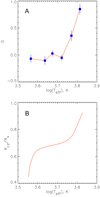 |
Fig. 7. Change in power index D with varying log of stellar effective temperature Teff (panel A) in comparison with the location of tachocline (panel B), revealed by the models of young (0.5 Gyr) MS stars with the solar abundance of metals (van Saders & Pinsonneault 2012). |
Based on the discovered separation of RTC types and their possible wave drivers with respect to the stellar Teff, the RTCs of the stars presented in Fig. 3 can be distinguished as follows. The varying activity index  of the star KIC 12365719 with P = 0.854 days and Teff = 3556 K, shown in Fig. 3A, and its power spectrum in Fig. 3B, represent an example of a Kelvin wave-driven RTC. The Rossby wave-driven modulation of the activity index takes place in the star KIC 7671028 with P = 15.623 days and Teff = 6675 K, shown in Fig. 3E (the power spectrum is shown in Fig. 3F). The approximately close to each other periods of RTCs on the stars KIC 12365719 and KIC 7671028 have in fact essentially different physical nature (i.e., wave drivers). At the same time, as can be seen in Figs. 3A and C, the fast rotating stars KIC 12365719 (P = 0.854 days, Teff = 3556 K) and KIC 8144578 (P = 0.593 days, Teff = 6641 K) with approximately the same P, but different Teff show significant difference in Pcyc, which reflects the difference of their wave drivers. An important attribute of the shortest detected cycle with Pcyc ≈ 20 days on the star KIC 8144578, seen in the power spectrum in Fig. 3D, consists in its clustering in the packages with a duration of about 150 days, visible in the activity time series plot in Fig. 3C. This modulation looks similar to the Kelvin wave-driven RTC in Fig. 3A. This can be interpreted as a signature of joint modulation of the emergence of magnetic flux tubes in the stellar convection zone by Kelvin and Rossby waves, which results in the modulation of the shortest Kelvin wave-driven activity cycle by the longer Rossby wave periodicity.
An intermediate state of transition from the Kelvin wave-driven to Rossby wave-driven mechanism of RTCs takes place for the solar-type stars with the temperatures 5500 ≲ Teff ≲ 6000 K and D = 0.34 ± 0.09 shown in the diagram in Fig. 4. In particular, the deviating values of Ppeak < 100 days are demonstrated by fast rotators with P < 5 days, for which the increase of Rossby waves domination should be typical.
4. Conclusions
Our survey of short-period activity cycles in MS stars reveals that the phenomenon of RTCs is more complex than previously thought. Based on the performed analysis reported above, our conclusions can be summarized as follows.
1. The obtained information confirms the phenomenological analogy between the stellar RTCs and the solar Rieger cycles (see, e.g., Figs. 2 and 4, and discussion in Sect. 2.2).
2. Two types of RTCs can be distinguished: activity cycles with the period PRTC independent on the stellar rotation, which dominate on the stars with Teff ≲ 5500 K, and activity cycles with PRTC proportional to the stellar rotation period P, which take place on the stars with Teff ≳ 6300 K. These two types of RTCs can be driven by the Kelvin and Rossby waves, respectively.
3. The Rossby wave-driven RTCs show the relation with the location of tachocline at shallow deeps in the hot stars. This confirms the theoretical predictions of the connection of RTCs with tachocline (Zaqarashvili 2018; Gachechiladze et al. 2019). At the same time, the Kelvin wave-driven RTCs do not show such a connection.
4. At the same time, the duration of RTC on particular star cannot be used as a criterion to judge its physical nature as very similar PRTC on stars with different Teff and therefore different internal structures can be connected with different wave modes, and conversely different PRTC may have the same wave driver. Apparently, both kinds of RTC wave drivers seem to coexist, arguing for the joint modulation of the magnetic flux tube emergence by Kelvin and by Rossby waves.
In view of the discovered two types of RTCs connected with different wave drivers, and their different relations with the tachocline, a revision of the RTC theory is needed.
Acknowledgments
This work was supported by the projects I2939-N27 and S11606-N16 of the Austrian Science Fund (FWF). M.L.K acknowledges additionally grant No.075-15-2020-780 (GA No.13.1902.21.0039) of the Russian Ministry of Education and Science, RSF grant No 18-12-00080, and the project “Study of stars with exoplanets”, supported by grant No.075-15-2019-1875 from the government of Russian Federation.
References
- Arkhypov, O. V., Khodachenko, M. L., Güdel, M., et al. 2015a, A&A, 576, A67 [NASA ADS] [CrossRef] [EDP Sciences] [Google Scholar]
- Arkhypov, O. V., Khodachenko, M. L., Güdel, M., et al. 2015b, ApJ, 807, 109 [NASA ADS] [CrossRef] [Google Scholar]
- Arkhypov, O. V., Khodachenko, M. L., Güdel, M., et al. 2016, ApJ, 826, 35 [NASA ADS] [CrossRef] [Google Scholar]
- Arkhypov, O. V., Khodachenko, M. L., Lammer, H., et al. 2018a, MNRAS, 473, L84 [NASA ADS] [CrossRef] [Google Scholar]
- Arkhypov, O. V., Khodachenko, M. L., Lammer, H., et al. 2018b, MNRAS, 476, 1224 [CrossRef] [Google Scholar]
- Arkhypov, O. V., Khodachenko, M. L., Güdel, M., et al. 2018c, A&A, 613, A31 [CrossRef] [EDP Sciences] [Google Scholar]
- Bondar’, N. I., Katsova, M. M., & Livshits, M. A. 2020, Geomag. Aeron., 59, 832 [CrossRef] [Google Scholar]
- Boro Saikia, S., Marvin, C. J., Jeffers, S. V., et al. 2018, A&A, 616, A108 [NASA ADS] [CrossRef] [EDP Sciences] [Google Scholar]
- Distefano, E., Lanzafame, A. C., Lanza, A. F., Messina, S., & Spada, F. 2017, A&A, 606, A58 [NASA ADS] [CrossRef] [EDP Sciences] [Google Scholar]
- Feng, S., Yu, L., Wang, F., Deng, H., & Yang, Y. 2017, ApJ, 845, 11 [CrossRef] [Google Scholar]
- Gachechiladze, T., Zaqarashvili, T. V., Gurgenashvili, E., et al. 2019, ApJ, 874, 162 [CrossRef] [Google Scholar]
- Gurgenashvili, E., Zaqarashvili, T. V., Kukhianidze, V., et al. 2016, ApJ, 826, 55 [NASA ADS] [CrossRef] [Google Scholar]
- Jeffers, S. V., Mengel, M., Moutou, C., et al. 2018, MNRAS, 479, 5266 [NASA ADS] [CrossRef] [Google Scholar]
- Kitze, M., Akopian, A. A., Hambaryan, V., Torres, G., & Neuhäuser, R. 2017, Astron. Nachr., 338, 49 [CrossRef] [Google Scholar]
- Lou, Y.-Q. 2000, ApJ, 540, 1102 [NASA ADS] [CrossRef] [Google Scholar]
- Massi, M., Neidhöfer, J., Carpentier, Y., & Ros, E. 2005, A&A, 435, L1 [NASA ADS] [CrossRef] [EDP Sciences] [Google Scholar]
- McQuillan, A., Mazeh, T., & Aigrain, S. 2014, ApJS, 211, 24 [NASA ADS] [CrossRef] [MathSciNet] [Google Scholar]
- Olspert, N., Lehtinen, J. J., Käpylä, M. J., Pelt, J., & Grigorievskiy, A. 2018, A&A, 619, A6 [NASA ADS] [CrossRef] [EDP Sciences] [Google Scholar]
- Raphaldini, B., Seiji Teruya, A., Raupp, C. F. M., & Bustamante, M. D. 2019, ApJ, 887, 1 [CrossRef] [Google Scholar]
- Reinhold, T., Cameron, R. H., & Gizon, L. 2017, A&A, 603, A52 [NASA ADS] [CrossRef] [EDP Sciences] [Google Scholar]
- Rieger, E., Share, G. H., Forrest, D. J., et al. 1984, Nature, 312, 623 [Google Scholar]
- Silva, H. G., & Lopes, I. 2017, Astrophys. Space Sci., 362, 44 [CrossRef] [Google Scholar]
- Silverman, S. M. 1990, Nature, 347, 365 [CrossRef] [Google Scholar]
- Singh, Y. P., & Badruddin, S. G. 2017. Planet. Space Sci., 138, 1 [CrossRef] [Google Scholar]
- Sturrock, P. A., Fischbach, E., & Jenkins, J. H. 2011, Sol. Phys., 272, 1 [CrossRef] [Google Scholar]
- van Saders, J. L., & Pinsonneault, M. H. 2012, ApJ, 746, 16 [NASA ADS] [CrossRef] [Google Scholar]
- Vida, K., Oláh, K., & Szabó, R. 2014, MNRAS, 441, 2744 [NASA ADS] [CrossRef] [Google Scholar]
- Zaqarashvili, T. 2018, ApJ, 856, 32 [NASA ADS] [CrossRef] [Google Scholar]
- Zaqarashvili, T. V., Carbonell, M., Oliver, R., & Ballester, J. L. 2010, ApJ, 709, 749 [NASA ADS] [CrossRef] [Google Scholar]
All Figures
|
Fig. 1. Distribution of the analyzed stellar set in the (log(g),Teff)-plane, i.e., an analog of the HR diagram. The values of the stellar surface gravity log(g) and effective temperature Teff are from the newest version of Kepler Archive DR25 (MAST). |
| In the text | |
|
Fig. 2. Examples of RTC modulations in time series of activity index |
| In the text | |
|
Fig. 3. Oscillatory behavior of the activity index |
| In the text | |
|
Fig. 4. Distribution of the log(Ppeak) estimates vs. log of the stellar rotation periods P for the solar-type stars with 5500 < Teff < 6000 K. For comparison, the position of solar RTCs is indicated with a yellow circle which corresponds to Ppeak = 154 days according to Rieger et al. (1984). The bar denotes the total range of solar RTCs according to Feng et al. (2017). The red line shows the linear regression of the lower border set of the log(Ppeak) cluster, obtained for the minimum values of Ppeak (red crossed squares) defined for the sequential ten intervals of P. The gray area in the lower right corner of the plot indicates the detection limit zone for Ppeak, restricted by the Nyquist frequency (2P)−1. |
| In the text | |
|
Fig. 5. Distribution of the log(Ppeak) estimates vs. log(Teff) for the same subset of fast rotating stars with 1 < P < 4 days as processed by other methods in Arkhypov et al. (2015b). The red line shows the linear regression of the lower border set of the log(Ppeak) cluster, obtained for the minimum values of Ppeak (red crossed squares) defined for the sequential ten intervals of Teff. The green line shows linear regression of log(Pcyc(log(Teff))) obtained in Arkhypov et al. (2015b) by other methods. The detection limit zone for Ppeak, restricted by the Nyquist frequency (2P)−1 for the considered subset of fast rotators appears outside of the displayed frame. |
| In the text | |
|
Fig. 6. Same as the Fig. 4 diagrams of log(Ppeak) distribution vs. log(P), but for cold (panel A) and hot (panel B) stars with 3000 < Teff < 4000 K and 6300 < Teff < 7000 K, respectively. |
| In the text | |
|
Fig. 7. Change in power index D with varying log of stellar effective temperature Teff (panel A) in comparison with the location of tachocline (panel B), revealed by the models of young (0.5 Gyr) MS stars with the solar abundance of metals (van Saders & Pinsonneault 2012). |
| In the text | |
Current usage metrics show cumulative count of Article Views (full-text article views including HTML views, PDF and ePub downloads, according to the available data) and Abstracts Views on Vision4Press platform.
Data correspond to usage on the plateform after 2015. The current usage metrics is available 48-96 hours after online publication and is updated daily on week days.
Initial download of the metrics may take a while.