| Issue |
A&A
Volume 651, July 2021
|
|
|---|---|---|
| Article Number | A54 | |
| Number of page(s) | 12 | |
| Section | Extragalactic astronomy | |
| DOI | https://doi.org/10.1051/0004-6361/202140459 | |
| Published online | 13 July 2021 | |
Spectral state transitions in Circinus ULX5
1
Nicolaus Copernicus Astronomical Center, Polish Academy of Sciences, ul. Bartycka 18, 00-716 Warsaw, Poland
e-mail: smondal@camk.edu.pl
2
Astronomical Observatory Institute, Faculty of Physics, A. Mickiewicz University, Słoneczna 36, 60-286 Poznań, Poland
3
University of California, San Diego, Center for Astrophysics and Space Sciences, MC 0424, La Jolla, CA 92093-0424, USA
4
Departament de Física, EEBE, Universitat Politècnica de Catalunya, Av. Eduard Maristany 16, 08019 Barcelona, Spain
Received:
30
January
2021
Accepted:
26
April
2021
Context. We performed timing and spectral analyses of multi-epoch Suzaku, XMM-Newton, and NuSTAR observations of the ultraluminous X-ray source (ULX) Circinus ULX5 with the aim of putting constraints on the mass of the central object and the accretion mode operating in this source.
Aims. We investigate whether the source contains a stellar mass black hole (BH) with a super-Eddington accretion flow or an intermediate mass black hole accreting matter in a sub-Eddington mode. Moreover, we search for major observed changes in spectra and timing and determine whether they are associated with major structural changes in the disk, similarly to those in black hole X-ray binaries.
Methods. We collected all available broadband data from 2001 to 2018 including Suzaku, XMM-Newton, and NuSTAR. We a performed timing and spectral analyses to study the relation between luminosity and inner disk temperature. We proceeded with time-averaged spectral analysis using phenomenological models of different accretion modes. Finally, we constructed the hardness ratio versus intensity diagram to reveal spectral state transitions in Circinus ULX5.
Results. Our spectral analysis revealed at least three distinctive spectral states of Circinus ULX5 that are analagous to state transitions in Galactic black hole X-ray binaries. Disk-dominated spectra are found in high flux states and the power-law dominated spectra are found in lower flux states. The source was also observed in an intermediate state, where the flux was low, but the spectrum is dominated by a disk component. Over eighteen years of collected data, ULX5 appeared two times in the high, three times in the low, and two times in the intermediate state. The fastest observed transition was ∼seven months.
Conclusions. Our analysis suggests that the central object in Circinus ULX5 is a stellar mass BH (< 10 M⊙) or, possibly, a neutron star (NS) despite there being no detection of pulsations in the light curves. The fractional variability amplitudes are consistent with state transitions in Circinus ULX5, wherein higher variability from the power law-like Comptonized emission becomes suppressed in the thermal disk-dominated state.
Key words: accretion / accretion disks / stars: black holes / X-rays: binaries
© ESO 2021
1. Introduction
The biggest mystery of ultraluminous X-ray sources (ULXs) is the mass of the central compact object. These sources are extragalactic compact accreting objects, located outside the nuclei of galaxies, their luminosities typically exceed the Eddington luminosity of a typical 10 M⊙ black hole (BH) accretor. They have high values of X-ray brightness, Lx > 1039 erg s−1, and low inner disk temperature, kTin ∼ 0.1–0.3 keV, obtained from a spectral fitting of multicolor accretion disk (MCD) components. Consequently, ULXs have been suggested to be prime candidates for hosting intermediate-mass BHs (IMBHs), ∼102−4 M⊙ (Kaaret et al. 2003; Miller et al. 2004a,b). However, the notion of every ULX harboring an IMBH conflicts with population studies since this would imply too high an IMBH formation rate in star-forming galaxies (King 2004). Such a notion is also inconsistent with the break at ∼2 × 1040 erg s−1 in the luminosity function of point-like X-ray sources in star-forming galaxies (Swartz et al. 2004; Mineo et al. 2012).
A breakthrough discovery was made in 2014, when a pulsation with an average period of 1.3 s was measured in the NuSTAR data of M82 X-2 (Bachetti et al. 2014). Several subsequent discoveries of ULX pulsars (Fürst et al. 2016; Israel et al. 2017a,b; Brightman et al. 2018; Carpano et al. 2018; Sathyaprakash et al. 2019; Rodríguez Castillo et al. 2020) indicated that some ULXs have a neutron star (NS) as an accretor. The optical observations of a limited number of ULXs’ companions have revealed that they might belong to the class of high-mass X-ray binaries (Motch et al. 2011, 2014; Heida et al. 2015, 2016). These objects may comprise some fraction of the merging double compact objects that have been detected by the advanced instruments of LIGO and Virgo (Mondal et al. 2020a).
Due to the lack of a method for obtaining direct measurements of the compact object’s mass in ULXs, we can rely only on indirect procedures, for instance, by inferring the accretion mode of the source and comparing it to those of known sources. The most promising and straightforward test is to study the broadband spectra of ULXs, with the aim of deriving correlations between measurable global parameters. It is well known that in the case of Galactic black hole X-ray binaries (XRBs), if an observer has a direct view on the hot inner accretion disk, the standard model by Shakura & Sunyaev (1973; hereafter SS73) predicts a relation between luminosity and temperature:  (measured, e.g., by Gierliński & Done 2004). However, when the object is viewed close to edge-on, the source is visible through a disk wind photosphere that is measured to have a temperature of 0.1–0.3 keV.
The lower temperature value comes from the fact that when the source luminosity increases, the size of the photosphere becomes larger and its temperature drops. As demonstrated by King & Puchnarewicz (2002) and King (2009), this leads to an inverse luminosity relation in sources accreting at super-Eddington rates; King & Muldrew (2016) demonstrated that such thick disk winds can be produced in super-Eddington accreting ULXs.
This inverse correlation between disk luminosity and temperature has been observed in many individual ULXs after fitting phenomenological models as a MCD plus a power law to their broadband X-ray spectra (Feng & Kaaret 2007; Kajava & Poutanen 2009; Mondal et al. 2020b). Evidence for disk winds was also found in several ULXs via the detection of emission and absorption lines in high-resolution spectra (Middleton et al. 2014; Pinto et al. 2016, 2017; Walton et al. 2016; Kosec et al. 2018a,b). Thus, the combination of an inverse disk luminosity-temperature relation and the detection of a disk wind may support the notion that a given ULX source harbors a stellar-mass BH with super-Eddington accretion.
Another indirect constrain on BH mass in ULXs comes from X-ray spectral variability. It was found that some ULXs can represent different spectral states (for review see: Kaaret et al. 2017) in analogy with those observed in XRBs. Across the known population of ULXs, we can distinguish the following spectral states depending on X-ray luminosity.
At LX > 3 × 1039 erg s−1, sources display a so-called hard or soft UL state. The spectrum is fitted by two components: a soft excess and a hard component that shows a turnover at high energies. In the soft UL state, the soft component dominates the luminosity (Sutton et al. 2013).
At LX < 3 × 1039 erg s−1, we find the broadened disk (BD) state: A standard MCD model component is too narrow to fit the spectrum, and so it has to be broadened by a slim disk model or power-law component (Sutton et al. 2013).
Finally, a thermal spectrum with color temperature kT ∼ 0.1 keV and bolometric luminosity that is about a few times 1039 erg s−1, with almost no emission above 1 keV, are classified as supersoft UL (SSUL) state: Spectra are dominated by a low temperature blackbody component which enables production of over 90% of the intrinsic flux in the 0.3–10 keV band (Kong & Di Stefano 2003).
Some of the highest quality XMM-Newton spectra of a few tens of ULXs display a connection between the spectral state and accretion mode (Roberts 2007; Gladstone et al. 2009; Sutton et al. 2013): the BD state is usually observed in sources with lower luminosities, suggesting sub- or nearly Eddington accretion, while two-component UL states are seen in high-luminosity sources that strongly support super-Eddington accretion.
Furthermore, the majority of BD state objects do not display strong short timescale variability. The fact that only a few ULXs are strongly variable may be evidence that in those sources, a two-component hard/soft UL spectrum is present.
The UL state objects differ in their variability properties, such that hard UL spectra display lower levels of fractional variability (≪10%), while soft UL spectra are highly variable (10–30%). The difference in variability properties may be due to the wind opening angle, where geometrical beaming occurs, leading to eventual obscuration of hard radiation by the thick wind (Sutton et al. 2013). However, it is important to note that this behaviour is opposite to that seen in XRBs, where sources in the thermal-dominated spectral state exhibit lower variability than in the power law-dominated hard state (Churazov et al. 2001; Muñoz-Darias et al. 2011). Thus, the detection of a spectral state transition while tracking corresponding short time scale variability may indicate the accretion mode, and consequently, the BH mass in ULXs.
However, actual state transitions within individual sources have been poorly studied since multi-epoch observations are needed for this purpose. Until now, a single transition from soft-to-hard and hard-to-soft state was reported in the cases of IC 342 X-1 and IC 342 X-2, respectively (Kubota et al. 2001), and in the case of NGC 1313 X-1 (Feng & Kaaret 2006). Furthermore, the brightest ULX source in NGC 274 displayed a state transition between soft UL and SSUL, the latter representing a higher accretion rate (Feng et al. 2016; Pinto et al. 2021). For extreme super-Eddington accretion, blackbody emission may arise from the photosphere of a thick outflow and hard X-ray emission only emerges from the central low-density funnel. Until now, only Holmberg IX X-1 exhibited three spectral states, over a span of eight years (Luangtip et al. 2016), and most probably due to enhanced geometric beaming as the accretion rate increases and the wind funnel narrows; such changes cause the scattered flux from the central regions of the super-Eddington flow to brighten faster than the isotropic thermal emission from the wind. Thus, the detection of a state transition within an individual source may put constraints on the possible geometry of the emitting compact object.
In this paper, we aim to determine the nature of the compact object Circinus ULX5 and constrain its mass, as well as explore its accretion flow properties as a function of luminosity. To this end, we present a timing and spectral analysis of broad-band X-ray data of Circinus ULX5 from different epochs during 2001–2018 taken by Suzaku (Mitsuda et al. 2007), XMM-Newton (Jansen et al. 2001), and NuSTAR (Harrison et al. 2013). Our aim is to put tight constraints on the BH mass using all indirect methods described above. The paper is organized as follows: in Sect. 2 we describe the source and summarize its current status known from X-ray data. In the same section, we present the observations used in this paper and the data reduction processes. The next three sections contain results obtained from short timescale variability, the hardness-intensity diagram (HID), and broadband spectral analysis, respectively. We discuss our results in Sect. 6 and present our conclusions in Sect. 7.
2. Observations and data reduction
Circinus ULX5 is located on the outskirts of the Circinus galaxy, at α = 14h12m39s and δ = −65° 23′34″. The source was first detected in an XMM-Newton observation taken in 2001, and reported the ULX catalog of Winter et al. (2006) under the name Circinus XMM2. The source was interpreted to be in the so-called “high-state”, in which the thermal component dominates.
The first observations of ULX5 by the NuSTAR telescope were performed and analyzed by Walton et al. (2013). While the data taken in 2001 and 2006 by XMM-Newton indicated extreme flux variability, the later observation in 2013 did not show signatures of variability. Based on Suzaku observations in 2006 (Walton et al. 2013), ULX5 displays long term spectral evolution based on a clear correlation of hardness ratio with 0.5–10 keV luminosity. The increasing positive trend in the hardness-luminosity diagram is accompanied by 0.5–10 keV fractional variability amplitude reaching ∼12%. The source peak luminosity was calculated to reach a value of 1.6 × 1040 erg s−1 for a distance of ∼4 Mpc (Walton et al. 2013), measured with the Tully–Fisher method (Tully & Fisher 1977) when the Circinus galaxy (z = 0.001448) was discovered (Freeman et al. 1977). In X-ray spectral fits, depending on the model used, the values of Galactic neutral absorption toward the source range from 1 to 9.5 × 1021 cm−2. These values are consistent with the reported column densities NHI + NH2 ∼ (5.01 + 1.44)×1021 cm−2 of Galactic monatomic and diatomic hydrogen, respectively, toward the source by Willingale et al. (2013) and HI4PI Collaboration et al. (2016).
The details of X-ray observations we studied are given in Table 1. Henceforth in this paper we use the names of data sets listed in the first column of Table 1. Four data sets taken from 2014 to 2018 have been never published before. When calculating the luminosity, we accept the distance of 4.2 Mpc to the Circinus galaxy as discussed in Appendix A. We also studied the reflecting grating spectrometer’s (RGS) high resolution spectra taken in 2013, 2014, and 2018, but the data did not show any strong evidence for a disk wind; these data are presented in Appendix B.
Details of X-ray data analyzed in this paper.
2.1. XMM-Newton
We analyzed six XMM-Newton observations performed between 2001 to 2018, four of which had never been published before. The data reduction was done using XMM-Newton Science Analysis System (SASv16.0.0) following the online procedures. The first-order observation data files (ODF) were processed using emproc and epproc to create clean calibrated event files for the EPIC-MOS and EPIC-pn detectors, respectively. The source products were extracted from a circular region of 40″ radius and the background was selected from a source free region of size 80″. We used evselect to create the light curves and spectra. We allowed only single and double events for the EPIC-pn detector and single to quadruple events for both EPIC-MOS detectors. The source light curves were corrected for background counts using epiclccorr. We used rmfgen and arfgen to generate the redistribution matrix and auxiliary response files. We note that in some of the XMM-Newton observations, the EPIC-pn and MOS detectors were not observing simultaneously. This resulted in a variance in terms of the good time intervals (GTI) for the three detectors. Unfortunately, in the case of XMM-01, the observations with MOS-2 were taken in “partial window” mode; the source fell onto the outer part of the CCD and was read out, so no data on the ULX were collected.
2.2. Suzaku
We used Suzaku data taken in 2006 using the XIS (X-ray Imaging Spectrometer) CCDs (see Table 1, second row). The data reduction was performed using the HEASOFT software package. We used cleaned event files from the front-illuminated CCDs – XIS0, XIS2, and XIS3 – and back-illuminated CCD – XIS1, for both available editing modes, 3 × 3 and 5 × 5. We used xselect to extract the light curves and spectra. The source and background products were extracted from a circular region of 85″ in radius. The background was derived from regions that were free of other sources but in close proximity to the ULX. The attitude correction was performed with the use of the aeattcor2 standard FTOOL. We used the xisresp script to generate response matrix files, and the xisarfgen script to create auxiliary response files, for each detector and editing mode separately. We added all front-illuminated CCDs and, therefore, the total counts reported in Table 1 were combined from all three chips.
These data were published previously by (Walton et al. 2013) and the light curve presented in Fig. 9 of their paper clearly indicates a drop in flux by a factor of two, at around 40 ks into the observation. Therefore, for the purposes of the current paper, we extracted the Suzaku light curves and spectra from the first and second epochs of the observations: Suz-H-06 spanned the first 40.08 ks of the exposure, while Suz-L-06 spanned the last 67.94 ks. For the spectra of both epochs, we created combined spectra for the front-illuminated detectors (XIS023), using the FTOOL addascaspec. Furthermore, for both the XIS023 and back-illuminated XIS1 spectra, we combined 3 × 3 and 5 × 5 modes using the same FTOOL. The process of combining and subtracting lightcurves was performed using the XRONOS script lcmath.
2.3. NuSTAR
The field of the Circinus galaxy was observed by NuSTAR in 2013 and in 2016. The data reduction was done using the pipeline NuSTAR Data Analysis Software (NUSTARDAS v1.9.5 provided with HEASOFT). The unfiltered event files were cleaned and data taken during passages through the South Atlantic Anomaly were removed using nupipeline. The source products were extracted from a circular region of radius 70″ using nuproducts. The background was selected from a source free circular region of radius 100″.
3. Short timescale variability
Circinus ULX5 is an extremely variable ULX compared to other ULXs of similar luminosity, which typically do not show strong flux variability (Heil et al. 2009). Walton et al. (2013) found that ULX5 showed 0.5–10 keV fractional rms variability amplitudes (hereafter, Fvar; Edelson et al. 2002; Vaughan et al. 2003, especially Eqs. (10) and (B2) in the latter for variance and variance errors). of ∼12–15% during the 2001 XMM-Newton and 2006 Suzaku observations. In the 2013 XMM-Newton observation, however, Fvar dropped to < 2%.
We start our analysis with light curves. The average count rates in the EPIC-pn detector in the 0.5–10 keV band are 0.38, 0.54, and 1.22 ct s−1 for XMM-14, XMM-16 and XMM-18S, respectively. All lightcurves are re-binned to 500 s. Figure 1 shows the soft (0.5–2 keV) and hard (2–10 keV) light curves as well as the hardness ratio (2–10 keV/0.5–2 keV) for three unpublished data sets.
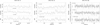 |
Fig. 1. Light curves extracted from the EPIC-pn detector, from data set XMM-14 (left panel), XMM-16 (middle panel), and XMM-18S (right panel). In each case, we present lightcurves for the soft (0.5–2 keV) and hard (2–10) keV bands (upper and middle panels, respectively) as well as the 2–10/0.5–2 keV hardness ratio (bottom panels). The light curves were re-binned to 500 s to yield a higher signal to noise ratio within each bin. |
Then for each epoch, we calculate Fvar in three spectral bands, 0.5–10, 0.5–2, and 2–10 keV. For longer observations, XMM-01, Suz-H-06, Suz-L-06, and XMM-18S, we chopped the lightcurves into 30 ks segments to ensure a more systematic comparison to the other observations. The Fvar was calculated from each segment separately and then averaged. The lightcurves have a time binning of 500 s, so Fvar gives the power spectrum integrated over the frequency range 3.33 × 10⁻⁵ Hz (1/30 ks) to 10−3 Hz (1/2 × 500 s). The variability amplitudes calculated for the total, soft, and hard bands for all eight data sets are listed in Table 2. The source shows 0.5–10 keV fractional excess variance at the ∼10–15% level during the XMM-01, Suz-H-06, Suz-L-06, XMM-14, XMM-16, and XMM-18F observations, whereas the value dropped to ∼2% in the XMM-13 and XMM-18S data, which is consistent with earlier studies. In the case of the XMM-18F light curves, only an upper limit on Fvar, could be measured; otherwise, Fvar could not be constrained.
Fractional variability amplitude, Fvar, obtained from the total (0.5–10 keV), soft (0.5–2 keV), and hard (2–10 keV) band light curves, for the data sets given in the first column.
4. Hardness-intensity diagram
In order to search for potential spectral state transitions, we plotted the count rate hardness ratio versus intensity diagram using the EPIC-pn lightcurves from all data sets. Again, we used light curves binned to 500 s, and then again using 0.5–2, 2–10, and 0.5–10 keV. Figure 2 shows the (2–10 keV)/(0.5–2 keV) count rate ratio (hardness) plotted against the total band 0.5–10 keV count rate (intensity). There are two distinct “islands” visible in the diagram, where the intensity differs by a factor of 4–5, and the hardness ratio in the extreme cases differs by 1. Furthermore, the XMM-16 data (green squares in Fig. 2) are a factor of two brighter than XMM-01, XMM-14 and XMM-18F at the same hardness ratio. Suzaku data are not included in this diagram since the difference between count rate of both instruments does not allow for a direct comparison; nevertheless the HID for the 2006 Suzaku data was published by Walton et al. (2013).
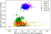 |
Fig. 2. Hardness ratio intensity diagram made from the EPIC-pn light curves. All data sets are arranged in two islands. |
It is evident from Fig. 2 that the observations have caught ULX5 at at least two distinct flux levels – a low flux level in 2001, 2014, and 2018 Feb., and a high flux level in 2013 and 2018 Sept. The transition between the observed flux levels is accompanied by a change in the 0.5–10 keV short timescale variability amplitude, which is larger than 10% at low flux, but drops to 2% at high flux. We additionally claim here that XMM-16 represents an intermediate flux state; we justify this conclusion based on a broadband spectral analysis of all data sets in Sect. 5, below.
5. Time-averaged spectral analysis
In the next step, we performed a time-averaged spectral analysis. Other than the Suzaku-06 data, which are divided into two time intervals (see Sect. 2.2), all spectra are averaged over the whole exposure. Each spectrum was grouped to a minimum of 20 counts in each energy bin. For the spectral modeling, we used the XSPEC v12.10.1 (Arnaud 1996), and for calculating correlations between parameters we used PYTHON environment. Spectral fitting was performed simultaneously for all detectors, using constant terms for cross calibration uncertainties and keeping them free for different detectors, but fixed to unity for EPIC-pn. For observations taken in 2013 and 2016, the XMM-Newton and NuSTAR data are simultaneous, thus allowing us to place better constraints on the continuum model between 0.5 and 20 keV. To account for Galactic absorption, all models are convolved with tbabs model available in XSPEC with updated solar abundances (Wilms et al. 2000). The fitting was performed using the χ2 statistic. The errors for each parameter are given at the 90% confidence level, allowing the other parameters to vary during error calculations. Whenever we fit several model components, we provide the normalization of each model component (see Tables 3 and 4). We note that for each model component, the normalization is defined in different ways and carries different physical meaning and units (see the XSPEC manual1).
Best-fit parameters obtained from the fits of each set of data.
Best parameters obtained from the fit of an accreting NS model to the XMM-16+NuSTAR-16 spectra.
5.1. Spectral state transitions
Figure 3 shows the XMM-Newton EPIC-pn and NuSTAR FPMB count spectra for different observational epochs for the purpose of comparing pn to pn and FPMB to FPMB only. Here, we do not include the Suzaku-06 data set since the difference between energy-dependent effective areas of the instruments does not allow us to trace spectral evolution in units of normalized counts. The color-coding is the same as in Fig. 2. Based on XMM-Newton data in Fig. 3, the same evolution is observed as in the hardness ratio intensity diagram, that is, a low flux level in 2001, 2014, and 2018 Feb., an intermediate flux level in 2016, and a high flux level in 2013 and 2018 Sept.
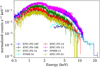 |
Fig. 3. Counts spectra from different epochs of observations obtained with the XMM-Newton EPIC-pn and NuSTAR FPMB detectors. The same spectral evolution is observed as in Fig. 2. |
A simple absorbed power-law model (hereafter pl) reveals curvature in the 2–10 keV band for data sets Suz-H-06, Suz-L-06,XMM-13+NuSTAR+13, XMM-16+NuSTAR+16, and XMM-18S, as shown in Fig. 4, where the data-to-model ratios for all observations are shown. This kind of “M-shaped” curvature has been seen in many other luminous ULXs (Stobbart et al. 2006; Gladstone et al. 2009). The curvature is present even if we allowed for a larger column density, significantly in excess of the Galactic value, which indicates the spectra are intrinsically curved. The curved residuals in the soft band, which are clearly visible when ULX5 is at the intermediate- and high-flux levels (Fig. 4), can be successfully modeled by a single-disk component. Moreover, data sets at a low flux level, XMM-01, XMM-14, and XMM-18F, are well fitted by the pl model and do not indicate more complex curvature.
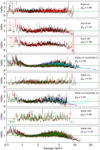 |
Fig. 4. Data-to-model ratio obtained from the fit of the tbabs*pl model to the data from all epochs marked at each panel. In the case of XMM-Newton, black, red, and green data points are from the EPIC-pn, MOS1, and MOS2 detectors, respectively. In the case of the Suzaku data, black points are from the front-illuminated XIS023 chips and red points are from the back-illuminated XIS1 chips. The blue and cyan points are from NuSTAR FPMA and FPMB, respectively. |
To model the spectral curvature over epochs, we fit a model comprised of two components, that is, the sum of a MCD model component represented by diskbb (Mitsuda et al. 1984; Makishima et al. 1986) and the pl model. All model parameters obtained from this fit are given in Table 3, where the fit statistic is given in the last column. We can observe a substantial fit improvement in cases where “M-shaped” data are presented in Fig. 4; namely, for Suz-H-06, Suz-L-06, XMM-13+NuSTAR-13, and XMM-18S, values of  have dropped from ≥1.38 to ≤1.08. The improved residuals are displayed in Fig. 5. Only XMM-16+NuSTAR-16 data still display a hard energy excess after removing the soft energy spectral curvature. Further discussion of this data set is presented in Sect. 5.3.
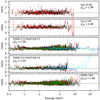 |
Fig. 5. Data-to-model ratio obtained from the tbabs*(diskbb+pl) model fit for the high and intermediate flux levels. A significant improvement in the residuals is visible compared to a single power-law model fit. |
To display the long-term spectral evolution of Circinus ULX5, we plot the absorbed best-fit model for each epoch in Fig. 6. It is clearly visible that the XMM-01, XMM-14 and XMM-18F data sets appear to be flat, consistent with an absorbed pl-like continuum, with negligible contribution from the disk. Those data sets are located in the lower island of the HID (Fig. 2) and indicate rather high fractional variability amplitudes, Fvar > 10% (Table 2). The total unabsorbed X-ray luminosity for those observations ranges from 4.45 up to 7.3 × 1039 erg s−1, placing these observations in a hard/low UL state.
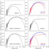 |
Fig. 6. Absorbed total model diskbb+pl (solid lines) fitted to the data from each epoch for the classification of spectral states. The disk component, diskbb, is also plotted with a dashed line. The source clearly evolves between a pl dominated state observed during 2001, 2014, and 2018 Feb. and a disk-dominated thermal state observed in 2006, 2013, 2016, and 2018 Sept. |
In contrast, other spectra such as those for the Suz-H-06, Suz-L-06, XMM-13+NuSTAR-13, XMM-16+NuSTAR-16, and XMM-18S data sets clearly show disk-dominated spectra with higher luminosities. But again we can divide them onto two groups: one with luminosities ranging from 7.7 up to 11 × 1039 erg s−1 in the cases of XMM-16+NuSTAR-16, Suz-L-06 and Suz-H-06, and from 16 up to 18.0 × 1039 erg s−1 in the cases of XMM-13+NuSTAR-13 and XMM-18S. We suggest that the first group represents the so-called intermediate soft state between high and low states, and the second group represents a typical high/soft UL state.
The evolution of the unabsorbed flux of Circinus ULX5, from the fitting of diskbb+pl model, is presented in Fig. 7. The evolution goes from the high state in 2013 to the low state in 2014, then to the intermediate state in 2016, to the low state in 2018 Feb., and to the high state in 2018 Sept., with all the observed states occurring within ∼5 years. The smallest observed timescale for a spectral state transition, is seven months. Another relatively fast transition is when the source transitions from high (2013) to low (2014) within 11 months. However, additional multi-epoch data obtained with a more dense sampling are needed to put better constraints on rapid transition timescales.
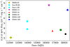 |
Fig. 7. Multi-epoch long-term flux variability of Circinus ULX5, for all data analyzed in this paper. |
5.2. Accretion mode in ULX5
We also check if the slim disk model, diskpbb (Abramowicz et al. 1988; Watarai et al. 2000), can improve our fit, thus indicating nearly-Eddington accretion. The slim disk model gives a flatter effective temperature radial profile, that is, the index p in the relation T(r) ∝ r−p is lower than 0.75, the latter being a typical value for the standard accretion disk SS73 model. For each epoch of our data, we obtain the best-fit value for the p parameter as listed in Table 3. These values are all < 0.75. Interestingly, when the source is in the low state (XMM-01, XMM-14, XMM-18F) p is 0.50 ± 0.01, 0.50 ± 0.02 and  , respectively; for the intermediate state (Suz-L-06, Suz-H-06, XMM-16), p is
  ,
,  and
and  , respectively; for the high state (XMM-13, XMM-18S), p is 0.64 ± 0.01 and 0.68 ± 0.01, respectively. Such a result is consistent with the notion that a super-Eddington accretion flow in an advection-dominated slim disk can explain the properties of ULX5. Furthermore we noticed that as the total flux increases, the values of p move towards 0.75, which is the value from the standard thin disk model. This movement may indicate that the slim disk model is a good description for relatively low-luminosity ULXs with near or above super-Eddington accretion, as pointed out by Sutton et al. (2013).
Finally, we tested a two-component model accounting for thermal Comptonization in a hot plasma near the accretion disk, namely, diskbb plus nthcomp (Zdziarski et al. 1996; Życki et al. 1999). All model parameters obtained from this fit are given in Table 3. In general, two-component models such as diskbb+pl and diskbb+nthcomp yield slightly better test statistics than diskpbb, as seen at the last column of Table 3. We checked the Akaike Information Criterion (AIC Akaike 1973; Sugiura 1978) to compare the models. The AIC information tells us that the diskbb+nthcomp model better describes the data than diskbb+pl model in the cases of the XMM-01, Suz-H-06, and Suz-L-06 data sets, but it is the opposite in the cases of the XMM-13, XMM-16 and XMM-18S data sets. For XMM-14 and XMM-18F, these two models are indistinguishable. Furthermore, in two cases (XMM-16+NuSTAR-16, XMM-18F), the electron temperature is not fully constrained, which may indicate that either the model is inefficient or we have too few data points at higher energies.
To put a better constraint on the accretion mode operating in ULX5, we determined the inner disk radius, Rin, and the corresponding inner disk temperature, Tin, and their evolution over different epochs. One can estimate the value of Rin from the normalization of the diskbb component, if the distance to the source and the viewing angle are known. The normalization of the diskbb component is (rin/D10)2cos(θ), where D10 is the distance to the source in units of 10 kpc, θ is the viewing angle, and rin is the apparent inner disk radius, that is, without accounting for the color-correction factor. The inner disk radius after color-correction is given by Rin = ξκ2rin, where we used  and κ = 1.7 (Kubota et al. 1998). To do so, we need the disk component to be strongly visible in the data, otherwise the fitting can lead to parameter degeneracy between Tin and the diskbb model normalization. For our data, we estimated Rin assuming the distance to the source is 4.2 Mpc and the source is viewed face-on (i.e., θ = 0).
Figure 8 shows the estimated inner disk radius from the diskbb+pl and diskbb+nthcomp model fittings. The inner disk radius and temperature follows an inverse relation,  . In general, as the source flux increases, the inner disk temperature increases and the inner disk radius decreases. We compare the inferred values of radius to the innermost stable circular orbit (ISCO) radius of a non-rotating 10 M⊙ BH. When the source is in a clearly pl-dominated hard/low spectral state, namely, for XMM-14 and XMM-18F, the inner disk radius is about 400 gravitational radii, RG, which is a very large value, but the weakness of the disk component in these data do not allow us to constrain this parameter well. For almost all other data sets, the disk goes down to the ISCO, although there are three points where, in the case of diskbb+pl, Rin goes below 6 RG. Such a scenario can be realized in the case of a maximally pro-grade rotating BH, when ISCO radius can be brought down from 6 to 1.2 RG, or in the case when the mass of the central object is even lower than 10 M⊙. The distribution of inner disk radii provides the value of Tin, which, in disk-dominated spectral states, is quite high, namely, ∼1–2 keV. This value comparable to those observed in XRBs, making Circinus ULX5 particularly notable and distinct from the rest of the ULXs.
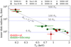 |
Fig. 8. Relation between disk Rin and Tin obtained from a spectral fitting of two models, diskbb+pl and diskbb+nthcomp, with data shown in red and green, respectively. The relation |

Nevertheless, both models presented in Fig. 8 represent geometrically thin sub-Eddington accretion disk whereas the normalization of the diskbb component suggests a lower-mass BH. To account for super-Eddington accretion indicated by high luminosity, we constructed a more physically consistent model composed of diskbb component for the outer sub-Eddington part of the disk, which is accounted for only the low energy curvature, plus the diskpbb component for the inner super-Eddington part of the disk that fits the high energy component. The fitting parameters are given in Table 3, and in Table 4 in the case of 2016 data set. Then in Fig. 9 we plot the inner disk radius and temperature relation from the diskpbb model component. The absence of the high energy curvature in three data sets observed during low states (XMM-01, XMM-14, and XMM-18F) leads to a high inner-disk temperature and very low inner-disk radius, which is even lower than the ISCO radius of a maximally spinning 10 M⊙ BH. On the other hand, the inner disk radius obtained from the high flux data sets lies just below 6 RG.
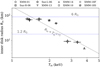 |
Fig. 9. Relation between disk Rin and Tin (i.e., |

Next, in Fig. 10, we plot unabsorbed 0.1–50 keV disk flux (the allowed limit in XSPEC for the diskpbb model) versus the inner disk temperature obtained from the same diskpbb model component. In the standard regime, where the value of Rin obtained from the disk component normalization remains constant, the disk flux should follow  (Kubota et al. 2002) for thin accretion disk and
  for advection dominated slim accretion disk. From this figure we excluded observations where Tin is not properly constrained due to the absence of a clear disk component, and which led to the smaller values of inner disk radius shown in Fig. 9. If we fit the data points ignoring the XMM-01, XMM-14, and XMM-18F data sets, the scaling relation becomes
  . This is clearly what we would expect from the advection dominated accretion mode where the correlation power goes to ∼2. This also demonstrates that we have a direct view of accreting matter that is not covered by the disk wind, since the flux temperature correlation power is positive (for more on the opposite result, see: Feng & Kaaret 2007; Kajava & Poutanen 2009; Mondal et al. 2020b).
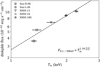 |
Fig. 10. diskpbb flux versus Tin relation inferred from a spectral fitting of the diskbb+diskpbb model. Only soft thermal disk-dominated spectra were used. The dashed black line shows the best fit to the data points. |
5.3. XMM-16 and NuSTAR-16 data set
During the 2016 observation, the emission above 10 keV was extremely weak, but the NuSTAR spectrum shows a rollover above 10 keV. The 0.5–10 keV EPIC-pn mean count rate was 0.53 ct s−1, whereas during 2013 it was 1.25 ct s−1. Figure 11 clearly demonstrates that the 0.5–20 keV spectrum cannot be fitted by a single accretion disk model (neither diskbb nor diskpbb). Adding an extra pl or nthcomp component to the diskbb model improves the fit significantly, but the ratio plot still shows a hard excess at higher energies. Furthermore, Walton et al. (2018) compared the hard excess of the 2013 broadband 0.3–30 keV data set to the hard excess present in ULX pulsars M82 X-2, NGC 7793 P13, and NGC 5907 ULX and conclude that the hard excess is consistent with being produced by an accretion column.
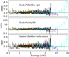 |
Fig. 11. Data-to-model ratio obtained from various model fits to the XMM-16 and NuSTAR-16 data set. Black, red, green, blue, and cyan denote the data from EPIC-pn, MOS1, MOS2, FPMA, and FMPB, respectively. |
Therefore, we constructed a phenomenological accreting NS model, similar to that of Walton et al. (2018), to fit the 2016 broadband 0.5–20 keV data. The model is composed of a thin disk model, diskbb, for the outer sub-Eddington part of the disk up to the spherization radius Rsph plus the slim disk model diskpbb for the inner super-Eddington part from Rsph to the inner magnetospheric radius Rm, and also includes a cut-off power-law model, cutoffpl, for emission from the accretion column. Due to the limited range of the broadband data, the energy cutoff is not well constrained; therefore we freeze Ecut at 10 keV, since the ULX pulsars have observed cutoff energies around 5–15 keV (Brightman et al. 2016; Israel et al. 2017b; Walton et al. 2018). We obtained an excellent fit, with χ2/dof = 585/557 or  . All fit parameters are given in Table 4
The resultant fit with the unfolded spectrum is shown in Fig. 12. The normalization of the accretion disk parameters gives radii of Rsph = 550 km and Rm = 73 km assuming the source was observed face-on and assuming the values of the color-correction factor mentioned previously. The spherization radius scales with mass accretion rate as  (Shakura & Sunyaev 1973); equating this with the value obtained from the fit and considering a NS of 1.4 M⊙, the mass accretion rate is Ṁacc ∼ 20 ṀEdd. Similarly, the magnetospheric radius scales with the dipole magnetic field strength and the source luminosity as
  cm where B12, L37 and M1.4 M⊙ are the magnetic field strength in units of 1012 G, the bolometric luminosity in units of 1037 erg s−1 and the mass of the NS in 1.4 M⊙ units, respectively (Lamb et al. 1973). Considering the 0.5–10 keV luminosity as a proxy for the bolometric luminosity, we obtained a lower limit on the strength of the magnetic field is > 5 × 10¹⁰ G.
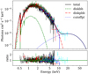 |
Fig. 12. Spectral fit to the XMM-16 and NuSTAR-16 data set. The total absorbed model is composed of diskbb for the outer sub-Eddington disk plus diskpbb for the inner super-Eddington disk and a cut-off power law (cutoffpl) for emission from the accretion column onto the neutron star. The color scheme of the data points is the same as in Fig. 11. |
6. Discussion
The spectral and timing studies of Circinus ULX5 supports state transitions between hard and low UL states, represented in the XMM-01, XMM-14, and XMM-18F data sets and well fitted by a power-law model, while the soft and high UL state, represented in XMM-13+NuSTAR-13 and XMM-18S and well fitted by a MCD + power-law model. Furthermore, those states are separated by an intermediate UL state, where the unabsorbed flux is only very roughly 50% higher than in the low state, but the spectrum is already dominated by the disk component, Suz-H-06, Suz-L-06, and XMM-16+NuSTAR-16. Finally, the HID displays two distinct “islands” – one for lower hardness ratio and lower luminosity and a second one for higher hardness and luminosity. The transition track is not the same as observed in XRBs, since we do not obtain typical “q” shape in the HID; rather, it looks more likely a HID diagram for an atoll source, that is, a NS with island and banana states (Altamirano et al. 2005; Church et al. 2014). It is, of course, possible that the ULX may cover other regions of the HID that have simply not been sampled by the limited number of observations obtained thus far. Nonetheless, we have noticed significant changes in spectral and variability characteristics between the “islands” on timescales of ∼7 months to several years. Such clear state transitions have never reported in case of any other individual ULX source. Our result strongly supports the finding that Circinus ULX5 switches between nearly- and super-Eddington modes of accretion around a stellar-mass BH or possibly a NS as well. We note that XRBs display much faster state transitions, on the order of days, and they can take typically months to trace out a complete evolution in the q-loop in the HID (e.g., the persistent XRB system Cyg X-1, Zhang et al. 1997). The differences in timescales between ULX5 and XRBs may originate from the fact that transient XRBs never become super-Eddingon, but we need more long term X-ray monitoring of Circinus ULX5 to fully resolve this issue.
The short-timescale variability behavior also correlates with the spectral evolution. The fractional variability amplitudes in the 0.5–10 keV band light curves is large (∼10–15%) when the source is in hard/low state, and it is small (∼2%) in the disk-dominated soft/high state. Galactic BH XRBs show similar behavior, with higher variability amplitudes associated with coronal emission in the hard and low state (Homan et al. 2001; Churazov et al. 2001; Muñoz-Darias et al. 2011). In general, ULXs do not show short-timescale variability (both flux and spectral) and most ULXs do not change over decades.
From our spectral fitting to multi-epoch data, we obtained an inverse inner disk radius versus temperature relation, with a power of –1.90 from the diskbb component normalization and −2.71 from the diskpbb component normalization. In the Rin − Tin diagram (Figs. 8 and 9), all inferred radii from disk-dominated spectra are near 6RG for a 10 M⊙ BH, except for the cases where the inner disk temperatures and radii are not properly constrained. The measured radii which are lying just below 6RG could be increased in value, if Circinus ULX5 would be observed at a higher inclination angle such as θ > 70°, that is, almost edge on. It is very unlikely that Circinus ULX5 is observed at such a high inclination angle because in this scenario, Circinus ULX5 would appear as a soft ULX with kTin ∼ 0.1–0.3 keV, in which most of the emission from the inner disk is intercepted by a wind. However, no strong wind was detected in the XMM-Newton RGS data (see Appendix B). Circinus ULX5 has a rather high inner disk temperature, close to 2 keV, despite its large luminosity.
Furthermore, the obtained disk flux and temperature relation shows a positive correlation with high index  . The best-fit value is not far from the typical
  relation expected from super-Eddington advection dominated accretion disk. Based on this finding, together with the quite high value of Tin (in the range of 1–2 keV; Fig. 10), it is most likely that the compact object in Circinus ULX5 is a low mass BH (< 10 M⊙), ruling out the hypothesis of IMBH.
It is also possible that Circinus ULX5 can host a NS. We have demonstrated in this paper that the XMM-16+NuSTAR-16 0.5–20 keV data can be well fitted by a three-component model composed of MCD emission for the outer sub-Eddington disk, slim disk emission for the inner super-Eddington disk, and a cut-off power law responsible for the emission from the accretion column onto NS. From such a fit, we can put rough constraints on the mass accretion rate, ∼20 ṀEdd, and on the strength of the magnetic field, > 5 × 10¹⁰ G. In addition, Różańska et al. (2018) obtained a very good fit by applying a single-model component made up of the emission from the NS surface plus the accretion disk emission to the broadband 0.3–30 keV 2013 data set. The fit is interesting to note since the distance to the source inferred from a spectral fitting of single model component agrees with other distance measurements (see Appendix A for discussion).
7. Conclusions
We analyzed multi-epoch observations of Circinus ULX5 taken with Suzaku, XMM-Newton, and NuSTAR from 2001 to 2018. We performed spectroscopy and timing analyses to obtain the physical properties of the source and compare them with theoretical models. The unabsorbed 0.5–10 keV luminosity of the source is extremely high: ∼1.8 × 1040 erg s−1. Our conclusions based on the timing analysis and various spectral fitting models are as follows:
-
The fitting of multi-epoch X-ray observations revealed three spectral states in which the source was observed: three observations caught the source in a hard and low UL, power law-dominated state; three observations caught the source in an intermediate state, with a disk-dominated spectrum but still relatively low flux; two observations caught the source in a soft and high disk-dominated state, where the flux had increased by a factor of four compared to the hard and low state. The minimum observed timescale for a spectral state transition was about seven months.
-
Circinus ULX5 exhibits short-timescale variability amplitudes that are correlated with spectral state. The 0.5–10 keV fractional variability amplitude Fvar is larger than ∼10–15% in the hard and low state, whereas in the thermal disk-dominated or high-flux state, variability is suppressed, and Fvar drops to ∼2%.
-
The normalization of the MCD model indicates that the inner disk radius is equal or slightly smaller than the ISCO for a non-spinning 10 M⊙ BH. This implies a stellar-mass compact object in Circinus ULX5. As we do not know the spin of the compact object, there is a possibility that central object can be highly spinning, but it is unlikely to be IMBH.
-
The flux and inner disk temperature follows a relation of
 for the two component diskbb plus diskpbb model and the inner disk radii obtained from the diskpbb normalization hints towards a small mass compact objects. These results strongly suggests that Circinus ULX5 accreting above the critical limit with a stellar mass compact accretor.
 -
The hard excess present in the broadband 0.5–20 keV XMM-16+NuSTAR-16 data can be interpreted as emission from the accretion column of a NS similar to that present in ULX pulsars. We constrain the mass accretion rate at ∼20 ṀEdd and the magnetic field strength to be > 5 × 10¹⁰ G for a 1.4 M⊙ NS, based on the fitting of a phenomenological model of super-Eddington accretion.
The whole data set is available under a different name for the galaxy: HIPASS J1413-65, on http://vizier.cfa.harvard.edu/viz-bin/VizieR.
Acknowledgments
AR was partially supported by Polish National Science Center grants No. 2015/17/B/ST9/03422, 2015/18/M/ST9/00541. BDM acknowledges support from Ramóny Cajal Fellowship RYC2018-025950-I. AGM was partially supported by Polish National Science Center grants 2016/23/B/ST9/03123 and 2018/31/G/ST9/03224. The work has made use of publicly available data from HEASARC Online Service, XMM-Newton Science Analysis System (SAS) developed by European Space Agency (ESA), and NuSTAR Data Analysis Software (NUSTARDAS) jointly developed by the ASI Science Data Center (ASDC, Italy) and the California Institute of Technology (USA). Software: Python (Van Rossum & Drake 2009), Jupyter (Kluyver et al. 2016), NumPy (van der Walt et al. 2011; Harris et al. 2020), matplotlib (Hunter 2007).
References
- Abramowicz, M. A., Czerny, B., Lasota, J. P., & Szuszkiewicz, E. 1988, ApJ, 332, 646 [Google Scholar]
- Akaike, H. 1973, Information Theory and an Extension of the Maximum Likelihood Principle (New York, NY: Springer), 199 [Google Scholar]
- Altamirano, D., van der Klis, M., Méndez, M., et al. 2005, ApJ, 633, 358 [NASA ADS] [CrossRef] [Google Scholar]
- Arnaud, K. A. 1996, in XSPEC: The First Ten Years, eds. G. H. Jacoby, & J. Barnes, ASP Conf. Ser., 101, 17 [Google Scholar]
- Bachetti, M., Harrison, F. A., Walton, D. J., et al. 2014, Nature, 514, 202 [NASA ADS] [CrossRef] [Google Scholar]
- Brightman, M., Harrison, F., Walton, D. J., et al. 2016, ApJ, 816, 60 [Google Scholar]
- Brightman, M., Harrison, F. A., Fürst, F., et al. 2018, Nat. Astron., 2, 312 [NASA ADS] [CrossRef] [Google Scholar]
- Carpano, S., Haberl, F., Maitra, C., & Vasilopoulos, G. 2018, MNRAS, 476, L45 [NASA ADS] [CrossRef] [Google Scholar]
- Cash, W. 1979, ApJ, 228, 939 [NASA ADS] [CrossRef] [Google Scholar]
- Churazov, E., Gilfanov, M., & Revnivtsev, M. 2001, MNRAS, 321, 759 [NASA ADS] [CrossRef] [Google Scholar]
- Church, M. J., Gibiec, A., & Bałucińska-Church, M. 2014, MNRAS, 438, 2784 [CrossRef] [Google Scholar]
- Edelson, R., Turner, T. J., Pounds, K., et al. 2002, ApJ, 568, 610 [NASA ADS] [CrossRef] [Google Scholar]
- Feng, H., & Kaaret, P. 2006, ApJ, 650, L75 [NASA ADS] [CrossRef] [Google Scholar]
- Feng, H., & Kaaret, P. 2007, ApJ, 660, L113 [CrossRef] [Google Scholar]
- Feng, H., Tao, L., Kaaret, P., & Grisé, F. 2016, ApJ, 831, 117 [NASA ADS] [CrossRef] [Google Scholar]
- Freeman, K. C., Karlsson, B., Lynga, G., et al. 1977, A&A, 55, 445 [NASA ADS] [Google Scholar]
- Fürst, F., Walton, D. J., Harrison, F. A., et al. 2016, ApJ, 831, L14 [NASA ADS] [CrossRef] [Google Scholar]
- Gierliński, M., & Done, C. 2004, MNRAS, 347, 885 [NASA ADS] [CrossRef] [Google Scholar]
- Gladstone, J. C., Roberts, T. P., & Done, C. 2009, MNRAS, 397, 1836 [NASA ADS] [CrossRef] [Google Scholar]
- Harris, C. R., Millman, K. J., van der Walt, S. J., et al. 2020, Nature, 585, 357 [CrossRef] [PubMed] [Google Scholar]
- Harrison, F. A., Craig, W. W., Christensen, F. E., et al. 2013, ApJ, 770, 103 [Google Scholar]
- Heida, M., Torres, M. A. P., Jonker, P. G., et al. 2015, MNRAS, 453, 3510 [NASA ADS] [CrossRef] [Google Scholar]
- Heida, M., Jonker, P. G., Torres, M. A. P., et al. 2016, MNRAS, 459, 771 [NASA ADS] [CrossRef] [Google Scholar]
- Heil, L. M., Vaughan, S., & Roberts, T. P. 2009, MNRAS, 397, 1061 [NASA ADS] [CrossRef] [Google Scholar]
- HI4PI Collaboration (Ben Bekhti, N., et al.) 2016, A&A, 594, A116 [NASA ADS] [CrossRef] [EDP Sciences] [Google Scholar]
- Homan, J., Wijnands, R., van der Klis, M., et al. 2001, ApJS, 132, 377 [NASA ADS] [CrossRef] [Google Scholar]
- Hunter, J. D. 2007, Comput. Sci. Eng., 9, 90 [NASA ADS] [CrossRef] [Google Scholar]
- Israel, G. L., Belfiore, A., Stella, L., et al. 2017a, Science, 355, 817 [NASA ADS] [CrossRef] [Google Scholar]
- Israel, G. L., Papitto, A., Esposito, P., et al. 2017b, MNRAS, 466, L48 [NASA ADS] [CrossRef] [Google Scholar]
- Jansen, F., Lumb, D., Altieri, B., et al. 2001, A&A, 365, L1 [NASA ADS] [CrossRef] [EDP Sciences] [Google Scholar]
- Kaaret, P., Corbel, S., Prestwich, A. H., & Zezas, A. 2003, Science, 299, 365 [NASA ADS] [CrossRef] [Google Scholar]
- Kaaret, P., Feng, H., & Roberts, T. P. 2017, ARA&A, 55, 303 [Google Scholar]
- Kajava, J. J. E., & Poutanen, J. 2009, MNRAS, 398, 1450 [NASA ADS] [CrossRef] [Google Scholar]
- Karachentsev, I. D., Karachentseva, V. E., Huchtmeier, W. K., & Makarov, D. I. 2004, AJ, 127, 2031 [Google Scholar]
- Karachentsev, I. D., Makarov, D. I., & Kaisina, E. I. 2013, AJ, 145, 101 [NASA ADS] [CrossRef] [Google Scholar]
- King, A. R. 2004, MNRAS, 347, L18 [NASA ADS] [CrossRef] [Google Scholar]
- King, A. R. 2009, MNRAS, 393, L41 [NASA ADS] [Google Scholar]
- King, A., & Muldrew, S. I. 2016, MNRAS, 455, 1211 [NASA ADS] [CrossRef] [Google Scholar]
- King, A. R., & Puchnarewicz, E. M. 2002, MNRAS, 336, 445 [CrossRef] [Google Scholar]
- Kluyver, T., Ragan-Kelley, B., Pérez, F., et al. 2016, in Positioning and Power in Academic Publishing: Players, Agents and Agendas, eds. F. Loizides, & B. Schmidt (IOS Press), 87 [Google Scholar]
- Kong, A. K. H., & Di Stefano, R. 2003, ApJ, 590, L13 [NASA ADS] [CrossRef] [Google Scholar]
- Koribalski, B. S., Staveley-Smith, L., Kilborn, V. A., et al. 2004, AJ, 128, 16 [NASA ADS] [CrossRef] [Google Scholar]
- Kosec, P., Pinto, C., Fabian, A. C., & Walton, D. J. 2018a, MNRAS, 473, 5680 [NASA ADS] [CrossRef] [Google Scholar]
- Kosec, P., Pinto, C., Walton, D. J., et al. 2018b, MNRAS, 479, 3978 [NASA ADS] [Google Scholar]
- Kubota, A., Tanaka, Y., Makishima, K., et al. 1998, PASJ, 50, 667 [NASA ADS] [CrossRef] [Google Scholar]
- Kubota, A., Mizuno, T., Makishima, K., et al. 2001, ApJ, 547, L119 [NASA ADS] [CrossRef] [Google Scholar]
- Kubota, A., Done, C., & Makishima, K. 2002, MNRAS, 337, L11 [NASA ADS] [CrossRef] [Google Scholar]
- Lamb, F. K., Pethick, C. J., & Pines, D. 1973, ApJ, 184, 271 [NASA ADS] [CrossRef] [Google Scholar]
- Luangtip, W., Roberts, T. P., & Done, C. 2016, MNRAS, 460, 4417 [NASA ADS] [CrossRef] [Google Scholar]
- Makishima, K., Maejima, Y., Mitsuda, K., et al. 1986, ApJ, 308, 635 [NASA ADS] [CrossRef] [Google Scholar]
- Middleton, M. J., Walton, D. J., Roberts, T. P., & Heil, L. 2014, MNRAS, 438, L51 [NASA ADS] [CrossRef] [Google Scholar]
- Miller, J. M., Fabian, A. C., & Miller, M. C. 2004a, ApJ, 614, L117 [NASA ADS] [CrossRef] [Google Scholar]
- Miller, J. M., Fabian, A. C., & Miller, M. C. 2004b, ApJ, 607, 931 [NASA ADS] [CrossRef] [Google Scholar]
- Mineo, S., Gilfanov, M., & Sunyaev, R. 2012, MNRAS, 419, 2095 [NASA ADS] [CrossRef] [Google Scholar]
- Mitsuda, K., Inoue, H., Koyama, K., et al. 1984, PASJ, 36, 741 [NASA ADS] [Google Scholar]
- Mitsuda, K., Bautz, M., Inoue, H., et al. 2007, PASJ, 59, S1 [NASA ADS] [CrossRef] [EDP Sciences] [Google Scholar]
- Mondal, S., Belczyński, K., Wiktorowicz, G., Lasota, J.-P., & King, A. R. 2020a, MNRAS, 491, 2747 [Google Scholar]
- Mondal, S., Różańska, A., Lai, E. V., & De Marco, B. 2020b, A&A, 642, A94 [CrossRef] [EDP Sciences] [Google Scholar]
- Motch, C., Pakull, M. W., Grisé, F., & Soria, R. 2011, Astron. Nachr., 332, 367 [NASA ADS] [CrossRef] [Google Scholar]
- Motch, C., Pakull, M. W., Soria, R., Grisé, F., & Pietrzyński, G. 2014, Nature, 514, 198 [NASA ADS] [CrossRef] [Google Scholar]
- Muñoz-Darias, T., Motta, S., & Belloni, T. M. 2011, MNRAS, 410, 679 [NASA ADS] [CrossRef] [Google Scholar]
- Pinto, C., Middleton, M. J., & Fabian, A. C. 2016, Nature, 533, 64 [NASA ADS] [CrossRef] [Google Scholar]
- Pinto, C., Alston, W., Soria, R., et al. 2017, MNRAS, 468, 2865 [NASA ADS] [CrossRef] [Google Scholar]
- Pinto, C., Soria, R., Walton, D., et al. 2021, MNRAS, 505, 5058 [CrossRef] [Google Scholar]
- Roberts, T. P. 2007, Ap&SS, 311, 203 [NASA ADS] [CrossRef] [Google Scholar]
- Różańska, A., Bresler, K., Bełdycki, B., Madej, J., & Adhikari, T. P. 2018, A&A, 612, L12 [CrossRef] [EDP Sciences] [Google Scholar]
- Rodríguez Castillo, G. A., Israel, G. L., Belfiore, A., et al. 2020, ApJ, 895, 60 [CrossRef] [Google Scholar]
- Sathyaprakash, R., Roberts, T. P., Walton, D. J., et al. 2019, MNRAS, 488, L35 [NASA ADS] [CrossRef] [Google Scholar]
- Shakura, N. I., & Sunyaev, R. A. 1973, A&A, 24, 337 [NASA ADS] [Google Scholar]
- Stobbart, A. M., Roberts, T. P., & Wilms, J. 2006, MNRAS, 368, 397 [NASA ADS] [CrossRef] [Google Scholar]
- Sugiura, N. 1978, Commun. Stat. Theory. Methods, 7, 13 [Google Scholar]
- Sutton, A. D., Roberts, T. P., & Middleton, M. J. 2013, MNRAS, 435, 1758 [NASA ADS] [CrossRef] [Google Scholar]
- Swartz, D. A., Ghosh, K. K., Tennant, A. F., & Wu, K. 2004, ApJS, 154, 519 [NASA ADS] [CrossRef] [Google Scholar]
- Tully, R. B., & Fisher, J. R. 1977, A&A, 500, 105 [Google Scholar]
- Tully, R. B., & Fisher, J. R. 1988, Catalog of Nearby Galaxies (Cambridge, UK: Cambridge University Press) [Google Scholar]
- Tully, R. B., Rizzi, L., Shaya, E. J., et al. 2009, AJ, 138, 323 [NASA ADS] [CrossRef] [Google Scholar]
- van der Walt, S., Colbert, S. C., & Varoquaux, G. 2011, Comput. Sci. Eng., 13, 22 [Google Scholar]
- Van Rossum, G., & Drake, F. L. 2009, Python 3 Reference Manual (Scotts Valley, CA: CreateSpace) [Google Scholar]
- Vaughan, S., Edelson, R., Warwick, R. S., & Uttley, P. 2003, MNRAS, 345, 1271 [NASA ADS] [CrossRef] [Google Scholar]
- Walton, D. J., Fuerst, F., Harrison, F., et al. 2013, ApJ, 779, 148 [NASA ADS] [CrossRef] [Google Scholar]
- Walton, D. J., Middleton, M. J., Pinto, C., et al. 2016, ApJ, 826, L26 [Google Scholar]
- Walton, D. J., Fürst, F., Harrison, F. A., et al. 2018, MNRAS, 473, 4360 [NASA ADS] [CrossRef] [Google Scholar]
- Watarai, K.-Y., Fukue, J., Takeuchi, M., & Mineshige, S. 2000, PASJ, 52, 133 [NASA ADS] [CrossRef] [Google Scholar]
- Willingale, R., Starling, R. L. C., Beardmore, A. P., Tanvir, N. R., & O’Brien, P. T. 2013, MNRAS, 431, 394 [NASA ADS] [CrossRef] [Google Scholar]
- Wilms, J., Allen, A., & McCray, R. 2000, ApJ, 542, 914 [Google Scholar]
- Winter, L. M., Mushotzky, R. F., & Reynolds, C. S. 2006, ApJ, 649, 730 [NASA ADS] [CrossRef] [Google Scholar]
- Zdziarski, A. A., Johnson, W. N., & Magdziarz, P. 1996, MNRAS, 283, 193 [NASA ADS] [CrossRef] [Google Scholar]
- Zhang, S. N., Cui, W., Harmon, B. A., et al. 1997, ApJ, 477, L95 [NASA ADS] [CrossRef] [Google Scholar]
- Życki, P. T., Done, C., & Smith, D. A. 1999, MNRAS, 309, 561 [NASA ADS] [CrossRef] [Google Scholar]
Appendix A: Distance to the source
We would like to call attention to the fact that the commonly accepted distance to the Circinus galaxy is 4.2 Mpc, as given by NASA Extragalactic Database2 (NED), derived with the use of the Tully-Fisher method (Tully & Fisher 1977). This method aims at finding the systemic velocity of a given galaxy by measuring the relation between global galaxian HI profile width versus absolute magnitude. The measurements of the line fluxes and optical magnitudes span a number of years and are collected in Extragalactic Distance Databases3 (EDD; Tully & Fisher 1988; Tully et al. 2009; Karachentsev et al. 2013), but the final distance does not agree with the distance derived by the Hubble relation with the use of the same radial velocities reported in the above EDD. Taking the value of radial velocity of the Circinus galaxy with respect to the Local Group (LG) to be 204 km s−1, the distance derived from Hubble relation, D = vLG/H0, is D = 2.8 Mpc, with the value of the Hubble constant H0 = 72 km s−1 Mpc−1 (Karachentsev et al. 2004).
Another distant measurement from the Hubble relation was provided by Koribalski et al. (2004), who reported the systemic velocity of the Circinus4 galaxy to be vsys = 434 km s−1. Knowing this value, the radial velocity with respect to the LG can be computed from the relation vLG = vsys + 300sin(l)cos(b), where l and b are galactic coordinates. In the case of the Circinus galaxy,  and
and  , yielding vLG = 209 km s−1, reported in the above database. Even accepting the recent value of H0 = 75 km s−1 Mpc−1, we get D = 2.78 Mpc. This distance value is consistent with that obtained by Różańska et al. (2018),
  Mpc, wherein a single emission component from a non-spherical system containing NS and accretion disk was fitted to the same observations as presented in Walton et al. (2013).
In this paper, we accept the distance of 4.2 Mpc to Circinus galaxy, bearing in mind that Tully-Fisher relation is not very precise. Nevertheless, we have checked that for lower values of distance, all luminosities reported in Table 1 become a factor of two lower, but while still keeping ULX5 in the regime of ultraluminous sources.
Appendix B: High-resolution RGS spectra
To search for evidence for disk-driven outflowing winds in Circinus ULX5, we analyzed spectra from the XMM-Newton reflecting grating spectrometers (RGS) to search for narrow emission and absorption lines from ionized species. For the RGS analysis, we utilized three long-exposure, on-axis observations of Circinus ULX5: XMM-13, XMM-14, and XMM-18S. To achieve a higher signal-to-noise ratio (S/N), we combined all first-order RGS1 and RGS2 spectra. Even though the spectra appear very noisy, we restrict ourselves to binning the data to a minimum of three counts per energy bin so that any possible the emission and absorption features do not smear out. As the data is not of excellent quality, it is impossible to do a detailed modeling considering the optical depth, ionization parameter, wind column density, outflow velocity, etc. However we can still search for the possible presence of line features by performing a simple Gaussian scan, focusing on the 0.5–1.5 keV band, in which the RGS detector is the most sensitive. The fitting was done using Cash statistics (Cash 1979) which utilizes the Poisson likelihood function, most suitable for low numbers of counts per bin. The scan was done by adding a narrow Gaussian with a fixed energy and width (only the normalization was kept free) to the continuum model, fitting, and checking if there is improvement in the value of the C statistic compared to the single power-law continuum model. We searched with a line centroid step size of 0.001 keV (1000 steps). For the width of the Gaussian line we tested two values of σ: 1 and 0.1 eV. The improvement in the C statistic as a function of energy is plotted in Fig. B.1 with positive and negative values of ΔC-stat denoting candidate emission and absorption-like features, respectively. The significance of the detection can directly obtained from the value of ΔC-stat (ΔC-stat = 4 = 95.5% confidence level), and there are multiple candidate features as shown in Fig. B.1, most notably emission lines at 0.727 and 0.819 keV; the former is consistent with the rest-frame energy of Fe L XVII 3s–2p, and the latter is in the vicinity of 0.826 keV, the rest-frame energy of Fe L XVII 3d–2p. However, this approach may overestimates the significance as it does not take into account the large number of trials. The actual significance should be estimated through Monte Carlo simulations. We utilized the simftest tool available in XSPEC; it generates simulated data sets based on the null hypothesis model (continuum emission only), and fits a Gaussian, yielding the value of ΔC-stat associated with fitting photon noise. We performed 1000 trials for each individual candidate line identified with ≥2σ confidence according to the ΔC-stat. The resulting significance values obtained via simftest are much lower compared to the ΔC-stat test and we cannot conclude that any of the candidate lines are real. The strongest visible lines achieve maximum significances of only 50.2% at 0.819 keV, 46% for the line at 0.727 keV, and 42.1% for the line at 0.532 keV.
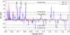 |
Fig. B.1. Result of the line search from the first-order RGS data by scanning the spectra using a narrow Gaussian. Positive and negative values of ΔC-stat denote candidate emission and absorption features, respectively. The F I K edge effect is instrumental in nature. |
All Tables
Fractional variability amplitude, Fvar, obtained from the total (0.5–10 keV), soft (0.5–2 keV), and hard (2–10 keV) band light curves, for the data sets given in the first column.
Best parameters obtained from the fit of an accreting NS model to the XMM-16+NuSTAR-16 spectra.
All Figures
|
Fig. 1. Light curves extracted from the EPIC-pn detector, from data set XMM-14 (left panel), XMM-16 (middle panel), and XMM-18S (right panel). In each case, we present lightcurves for the soft (0.5–2 keV) and hard (2–10) keV bands (upper and middle panels, respectively) as well as the 2–10/0.5–2 keV hardness ratio (bottom panels). The light curves were re-binned to 500 s to yield a higher signal to noise ratio within each bin. |
| In the text | |
|
Fig. 2. Hardness ratio intensity diagram made from the EPIC-pn light curves. All data sets are arranged in two islands. |
| In the text | |
|
Fig. 3. Counts spectra from different epochs of observations obtained with the XMM-Newton EPIC-pn and NuSTAR FPMB detectors. The same spectral evolution is observed as in Fig. 2. |
| In the text | |
|
Fig. 4. Data-to-model ratio obtained from the fit of the tbabs*pl model to the data from all epochs marked at each panel. In the case of XMM-Newton, black, red, and green data points are from the EPIC-pn, MOS1, and MOS2 detectors, respectively. In the case of the Suzaku data, black points are from the front-illuminated XIS023 chips and red points are from the back-illuminated XIS1 chips. The blue and cyan points are from NuSTAR FPMA and FPMB, respectively. |
| In the text | |
|
Fig. 5. Data-to-model ratio obtained from the tbabs*(diskbb+pl) model fit for the high and intermediate flux levels. A significant improvement in the residuals is visible compared to a single power-law model fit. |
| In the text | |
|
Fig. 6. Absorbed total model diskbb+pl (solid lines) fitted to the data from each epoch for the classification of spectral states. The disk component, diskbb, is also plotted with a dashed line. The source clearly evolves between a pl dominated state observed during 2001, 2014, and 2018 Feb. and a disk-dominated thermal state observed in 2006, 2013, 2016, and 2018 Sept. |
| In the text | |
|
Fig. 7. Multi-epoch long-term flux variability of Circinus ULX5, for all data analyzed in this paper. |
| In the text | |
|
Fig. 8. Relation between disk Rin and Tin obtained from a spectral fitting of two models, diskbb+pl and diskbb+nthcomp, with data shown in red and green, respectively. The relation |
| In the text | |
|
Fig. 9. Relation between disk Rin and Tin (i.e., |
| In the text | |
|
Fig. 10. diskpbb flux versus Tin relation inferred from a spectral fitting of the diskbb+diskpbb model. Only soft thermal disk-dominated spectra were used. The dashed black line shows the best fit to the data points. |
| In the text | |
|
Fig. 11. Data-to-model ratio obtained from various model fits to the XMM-16 and NuSTAR-16 data set. Black, red, green, blue, and cyan denote the data from EPIC-pn, MOS1, MOS2, FPMA, and FMPB, respectively. |
| In the text | |
|
Fig. 12. Spectral fit to the XMM-16 and NuSTAR-16 data set. The total absorbed model is composed of diskbb for the outer sub-Eddington disk plus diskpbb for the inner super-Eddington disk and a cut-off power law (cutoffpl) for emission from the accretion column onto the neutron star. The color scheme of the data points is the same as in Fig. 11. |
| In the text | |
|
Fig. B.1. Result of the line search from the first-order RGS data by scanning the spectra using a narrow Gaussian. Positive and negative values of ΔC-stat denote candidate emission and absorption features, respectively. The F I K edge effect is instrumental in nature. |
| In the text | |
Current usage metrics show cumulative count of Article Views (full-text article views including HTML views, PDF and ePub downloads, according to the available data) and Abstracts Views on Vision4Press platform.
Data correspond to usage on the plateform after 2015. The current usage metrics is available 48-96 hours after online publication and is updated daily on week days.
Initial download of the metrics may take a while.