| Issue |
A&A
Volume 651, July 2021
|
|
|---|---|---|
| Article Number | A80 | |
| Number of page(s) | 23 | |
| Section | Cosmology (including clusters of galaxies) | |
| DOI | https://doi.org/10.1051/0004-6361/202040239 | |
| Published online | 20 July 2021 | |
The MUSE-Faint survey
II. The dark-matter density profile of the ultra-faint dwarf galaxy Eridanus 2⋆
1
Leiden Observatory, Leiden University, PO Box 9513, 2300 RA Leiden, The Netherlands
e-mail: zoutendijk@strw.leidenuniv.nl
2
Instituto de Astrofísica e Ciências do Espaço, Universidade do Porto, CAUP, Rua das Estrelas, 4150-762 Porto, Portugal
3
Univ. Lyon, Univ. Lyon1, ENS de Lyon, CNRS, Centre de Recherche Astrophysique de Lyon UMR5574, 69230 Saint-Genis-Laval, France
4
Leibniz-Institut für Astrophysik Potsdam (AIP), An der Sternwarte 16, 14482 Potsdam, Germany
Received:
24
December
2020
Accepted:
24
April
2021
Aims. We use stellar line-of-sight velocities to constrain the dark-matter density profile of Eridanus 2, an ultra-faint dwarf galaxy with an absolute V-band magnitude MV = −7.1 that corresponds to a stellar mass M* ≈ 9 × 10⁴ M⊙. We furthermore derive constraints on fundamental properties of self-interacting and fuzzy dark matter scenarios.
Methods. We present new observations of Eridanus 2 from MUSE-Faint, a survey of ultra-faint dwarf galaxies with the Multi Unit Spectroscopic Explorer on the Very Large Telescope, and determine line-of-sight velocities for stars inside the half-light radius. Combined with literature data, we have 92 stellar tracers out to twice the half-light radius. With these tracers we constrain models of cold dark matter, self-interacting dark matter, and fuzzy dark matter, using CJAM and pyGravSphere for the dynamical analysis. The models of self-interacting and fuzzy dark matter relate the density profile to the self-interaction coefficient and the dark-matter particle mass, respectively.
Results. We find substantial evidence (Bayes factor ∼10−0.6) for cold dark matter (a cuspy halo) over self-interacting dark matter (a cored halo) and weak evidence (Bayes factor ∼10−0.4) for fuzzy dark matter over cold dark matter. We find a virial mass M200 ∼ 108 M⊙ and astrophysical factors J(αcJ) ~ 1011 M⊙2 kpc−5 and D(αcD) ~ 102 − 102.5 M⊙ kpc−2 (proportional to dark-matter annihilation and decay signals, respectively), the exact values of which depend on the density profile model. The mass-to-light ratio within the half-light radius is consistent with the literature. We do not resolve a core (rc < 47 pc, 68% confidence level) or a soliton (rsol < 7.2 pc, 68% confidence level). These limits are equivalent to an effective self-interaction coefficient fΓ < 2.2 × 10⁻²⁹ cm3 s−1 eV−1 c2 and a fuzzy-dark-matter particle mass ma > 4.0 × 10⁻²⁰ eV c−2. The constraint on self-interaction is complementary to those from gamma-ray searches. The constraint on fuzzy-dark-matter particle mass is inconsistent with those obtained for larger dwarf galaxies, suggesting that the flattened density profiles of those galaxies are not caused by fuzzy dark matter.
Key words: dark matter / galaxies: individual: Eridanus 2 / stars: kinematics and dynamics / techniques: imaging spectroscopy
© ESO 2021
1. Introduction
Over time, the astrophysical community has come to realize that baryonic matter and the established laws of physics are unable to explain our observations of the Universe. The discrepancy between baryonic and measured mass is almost universally interpreted as evidence for dark matter. The current paradigm, cold dark matter (CDM), has so far been able to explain our observations, albeit with a few open questions remaining. Various departures from the paradigm have been proposed with varying success, with the goal of addressing a perceived shortcoming of CDM or explaining the properties of dark matter as a consequence of a more physically motivated theory. The proposed alternatives to CDM span a wide range of masses and interactions, including weakly interacting massive particles (WIMPs; Steigman & Turner 1985), massive astrophysical compact halo objects (MACHOs; Griest 1991), axions (Weinberg 1978; Wilczek 1978; Preskill et al. 1983), warm dark matter (WDM) such as sterile neutrinos (Dodelson & Widrow 1994), and self-interacting dark matter (SIDM; Carlson et al. 1992; Spergel & Steinhardt 2000). Another option to solve the problem of ‘missing mass’, which has enjoyed less support, is to modify the laws of gravity instead of adding extra mass to the Universe. Examples of these modifications are modified Newtonian dynamics (Milgrom 1983) and emergent gravity (Verlinde 2017). In this paper we limit ourselves to a few different forms of dark matter.
The alternatives to CDM have different microphysical properties that lead to changes on astrophysical scales, making it possible in principle to distinguish between the individual alternatives and CDM through astronomical observations. One way of doing this is by investigating the gravitational interaction between the invisible dark matter and luminous objects. Different dark-matter theories often predict different spatial distributions of dark matter, which can be inferred from the kinematics of baryonic tracers. This kinematic approach is indirect but is complementary to the direct and indirect approaches that search for signatures such as annihilation and decay products. A complicating factor for astronomical observations is the complexity of astrophysical processes taking place in astronomical structures at the same time or in the past, which might also affect the measured spatial distribution of dark matter or the kinematics of the tracers.
Ultra-faint dwarf galaxies (UFDs) are perhaps the most promising class of objects for constraining dark matter on the basis of the density profile because these galaxies contain very little baryonic matter that could otherwise interfere with the interpretation of the results, both in a relative and an absolute sense: These galaxies are the most dark matter–dominated galaxies known (see e.g., McConnachie 2012) and contain very little luminous matter (MV > −7.7; Simon 2019). Baryonic effects are expected to be able to create significant cores in larger dwarf galaxies (Brooks & Zolotov 2014; Di Cintio et al. 2014a). Simulations of isolated galaxies show that the baryonic effects at play include bursty star formation, supernova feedback, and gas in- and outflows, or gravitational potential fluctuations in general (e.g., Read et al. 2016; El-Zant et al. 2016; Freundlich et al. 2020). Observational evidence that this process takes place in classical dwarf galaxies has been found by Read et al. (2019), who measure an anti-correlation between the dark-matter density at a radius of 150 pc and the stellar-mass/halo-mass ratio. In the case of UFDs, the baryonic content is so low that it is not expected to significantly alter the density profile from cuspy to cored (Peñarrubia et al. 2012; Oñorbe et al. 2015; Wheeler et al. 2019). However, other effects such as tides (Genina et al. 2020a) can also create cores in a CDM universe, and non-circular motions can bias kinematic analyses to make cusps appear as cores (Oman et al. 2019).
This paper is the second part in a series on MUSE-Faint, a survey of UFDs with the Multi Unit Spectroscopic Explorer (MUSE; Bacon et al. 2010) at the Very Large Telescope (VLT). In Zoutendijk et al. (2020, hereafter Paper I), we presented 4.5 h of observations on the central square arcminute of Eridanus 2 (Eri 2), a relatively bright UFD with absolute V-band magnitude MV = −7.1 (Crnojević et al. 2016). We found an intrinsic velocity dispersion of  for the bulk of the stars in the centre of Eri 2, whereas the central stellar over-density was found to have an intrinsic velocity dispersion of < 7.6 km s−1 (68% confidence level), supporting its earlier photometric classification as a star cluster (Crnojević et al. 2016).
The kinematics of larger dwarf galaxies are well studied. Fornax, Sculptor, and Draco, for example, have large sets of stellar line-of-sight velocities (Walker et al. 2009, 2015), and the latter two even have internal proper motion measurements (Massari et al. 2018, 2020). The profile of Fornax has been established as cored (e.g., Goerdt et al. 2006; Walker & Peñarrubia 2011; Amorisco et al. 2013), whereas Draco is generally regarded as having a cuspy density profile (e.g., Jardel et al. 2013; Read et al. 2018; Massari et al. 2020). There is no consensus on the density profile of Sculptor, with some authors preferring cores (e.g., Battaglia et al. 2008; Walker & Peñarrubia 2011), some preferring cusps (Richardson & Fairbairn 2014; Massari et al. 2018), and others claiming either profile fits the data (e.g., Breddels et al. 2013; Strigari et al. 2018). However, Read et al. (2019) note that the enclosed mass estimates for Sculptor are in agreement, the largest tension being ∼2σ.
Far less kinematic data is available for UFDs. The first UFD for which a velocity dispersion was determined was Ursa Major I (Kleyna et al. 2005). Currently, velocity dispersions are known for over half of the confirmed and candidate UFDs (Simon 2019). These measurements can be converted to mass estimates, for example by using the estimators from Wolf et al. (2010). Constraining a density profile for a UFD has so far not been possible due to the small sizes of the kinematic datasets and the limited radial ranges covered. However, the presence of the star cluster in Eri 2 has been used to argue for its hosting a cored profile (Amorisco 2017; Contenta et al. 2018).
Even without knowing the full density profile, classical and ultra-faint dwarf galaxies can be used to constrain dark-matter properties. If dark matter annihilates or decays, dark-matter haloes will emit radiation. Dwarf galaxies are promising targets because of their high dark-matter density and low radiation of baryonic origin. The annihilation and decay signals are proportional to the astrophysical J and D factors, which are integrated measures of the density profile. These factors are necessary to convert observed fluxes or flux limits to dark-matter properties. A number of studies have determined one or both of the astrophysical factors for dwarf galaxies (e.g., Bonnivard et al. 2015a; Fermi-LAT Collaboration 2014; Alvarez et al. 2020).
Here we present additional observations from MUSE-Faint on four new pointings surrounding the centre, roughly covering the half-light radius of Eri 2, R1/2/D = 2.31 ± 0.12 arcmin, at distance D = 366 ± 17 kpc, or R1/2 = 277 ± 14 pc (Crnojević et al. 2016). With these new fields, in combination with our central field and results at larger distances from the centre from another study (Li et al. 2017), we can study the kinematics of stars in Eri 2 over a wide range of radii. Using different kinematical analysis techniques, we put constraints on the dark-matter density profile of Eri 2, specifically whether the profile is cuspy or cored and to what degree, and translate these to constraints on the properties of dark-matter candidates: the self-interaction coefficient of SIDM and the dark-matter particle mass of fuzzy dark matter (FDM). Furthermore, we compare different models to one another using Bayesian evidence in an attempt to constrain which kinds of dark matter fit the data better. In the figures in this paper, each density profile model is consistently shown with the same colour to facilitate recognition and association.
In Sect. 2 we describe our data and its reduction (Sect. 2.1), the dark-matter density profile models (Sect. 2.2), and the analysis methods (Sects. 2.3 and 2.4). We continue in Sect. 3 with our results on dark-matter parameter constraints (Sect. 3.1), density-profile recovery and derived halo properties (Sect. 3.2), and a comparison of the evidence for the different dark-matter models (Sect. 3.3). We end with a discussion in Sect. 4 and our conclusions in Sect. 5.
2. Methods
We begin by describing our observations of Eri 2 from the MUSE-Faint survey, the data reduction, and the extraction of kinematics in Sect. 2.1. This is followed in Sect. 2.2 by the presentation of the three main dark-matter models tested in this paper. The parameters of the density profiles associated with these models are linked to the microphysical properties of dark matter. To constrain the profiles and thereby these properties, we used two analysis tools, CJAM and pyGravSphere, which are introduced in Sects. 2.3 and 2.4.
2.1. Observations and data reduction
The data were taken with VLT/MUSE during five guaranteed-time observing runs between October 2017 and December 2019. The estimated natural seeing varied between 0.6 and 1.0 arcsec, with adaptive optics reducing the seeing by 0.1–0.2 arcsec under good conditions. In Paper I we described the data reduction and source selection for Field 1, our central pointing on Eri 2. We used the same procedure independently on Fields 2 through 5, presented here for the first time (see Fig. 1).
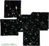 |
Fig. 1. Composite-colour image mosaic of Eridanus 2 as observed with MUSE-Faint. Sloan Digital Sky Survey filters g, r, and i were used for the colours blue, green, and red, respectively. Images of the five separately reduced fields were combined with Montage, and the colours were composited using the algorithm from Lupton et al. (2004). The 72 member stars with MUSE-Faint measurements are circled in green. Celestial north is up. The angular and physical scales at the distance of Eridanus 2 are indicated in the bottom left corner. |
In brief, we mostly followed the standard procedure of reducing MUSE data with the MUSE Data Reduction Software (DRS; version 2.4 for Field 1 and version 2.6 for Fields 2 through 5; Weilbacher et al. 2020), the exceptions being the use of the bad-pixel table from Bacon et al. (2017) and an auto-calibration step on a source-masked version of the cube. The DRS-produced data cubes were post-processed with Zurich Atmosphere Purge (ZAP; version 2.0; Soto et al. 2016) to remove residual sky signatures. We extracted spectra from these data cubes using PampelMuse (Kamann et al. 2013) and measured seeing full widths at half-maximum between 0.53 and 0.66 arcsec at 7000 Å for the five data cubes, using public Hubble Space Telescope data1 to construct a source catalogue. We used spexxy (version 2.5; Husser 2012) with the PHOENIX library of synthetic stellar spectra to determine line-of-sight velocities and made a catalogue of the results for each field. To ensure reliable velocity measurements and to limit contamination from background galaxies and Milky Way stars, we imposed a set of selection criteria: We removed catalogue entries that had a clearly extra-galactic spatial or spectral appearance, a spectral signal-to-noise ratio below 5, an unsuccessful velocity fit, a parallax measurement from Gaia Data Release 2 (Gaia Collaboration 2016, 2018; Lindegren et al. 2018) inconsistent with zero, or photometry inconsistent with a broadened MIST isochrone (Dotter 2016; Choi et al. 2016; Paxton et al. 2011, 2013, 2015). We had 95 entries that passed these criteria in the five catalogues. To this we added another catalogue with 47 observations of 28 member stars identified by Li et al. (2017), bringing the total number of entries to 142.
Since the six catalogues have some overlap on the sky, some sources occur in multiple catalogues. While merging the six source catalogues, we took into account the presence of these duplicate entries, which share an identifier, by replacing them with a single entry in the final catalogue. In this final catalogue we took the mean values of the right ascensions and declinations, the uncertainty-weighted mean values of the line-of-sight velocities, the sum in quadrature of the inverse uncertainties on the line-of-sight velocities, and the sum in quadrature of the signal-to-noise ratios. After this removal of duplicates, we were left with 109 unique stars. As in Paper I, we checked for possible remaining contamination of our sample by Milky Way stars by computing the membership probabilities of the selected sources. This we did by calculating the likelihood of observing the measured stellar velocities given two distribution functions – a Gaussian representing Eri 2 and a contaminating distribution based on the Besançon model of the Milky Way – and a membership probability for each star that weights the contributions of both distribution functions. The membership probabilities were determined by optimizing the likelihood while marginalizing over the mean velocity and dispersion of Eri 2. We found that ten of our sources had significantly lower membership probabilities than the others, leading to their exclusion from our sample and thus leaving us with 99 stars.
In Paper I we found that the Eri 2 cluster seen at the centre of this galaxy has a different kinematic distribution than the bulk of Eri 2. Moreover, it is still not completely clear how far this cluster is located from the centre of Eri 2 as we can only see the projected location. This leads to the question of whether the kinematics of the stars that make up the cluster are good tracers of the potential of Eri 2 or whether they mainly trace the properties of the star cluster itself. To avoid a possible bias in our results, we excluded the seven cluster member stars identified in Paper I from our sample, bringing our final selection to 92 stars. We present the positions and kinematics of the final selection in Table A.1. Of the final selection, 64 stars have only MUSE-Faint measurements, 20 stars have only measurements from Li et al. (2017), and eight stars have measurements from both sources.
2.2. Models of dark-matter density profiles
With the goal of placing constraints on the nature of dark matter, we compared our kinematic data to several models of dark-matter density profiles, each based on a different type of dark matter. As a null hypothesis, we used a Navarro–Frenk–White (NFW; Navarro et al. 1996) profile to represent CDM:
where ρ0 is known as the characteristic density and rs is the scale radius. We compared this with two other models: SIDM and FDM. The latter two models behave like an NFW profile on large scales but deviate on smaller scales. The extent of the deviation depends on the effective self-interaction coefficient in the case of SIDM and on the mass of the dark-matter particle in the case of FDM. Therefore, for both the SIDM and FDM models, not only can we compare one dark-matter theory to the other, but we can also place constraints on the properties of dark-matter particles under the assumption of the particular theory.
Self-interacting dark matter describes a form of dark matter that interacts with itself more strongly than with other particles (Spergel & Steinhardt 2000). Interactions that remove dark-matter particles from the halo according to the relation
where Γ is the self-interaction coefficient, produce a density profile
where ρc is the core density and rc is the core radius (Lin & Loeb 2016). We discuss how Γ and our constraints thereon relate to the cross-section σ in Sect. 4. The self-interaction described covers scattering and annihilation but has been designed with mainly the latter in mind. The profile can also be written as
with characteristic density ρ0 = ρc(rc/rs). The SIDM profile is equal to the CDM (NFW) profile for rc = 0, but for rc > 0 it exhibits a core instead of a cusp. Evidence in favour of the SIDM profile over the CDM profile would indicate that the density profile of Eri 2 is cored. If the density profile of Eri 2 is cuspy, both the CDM and SIDM models should be able to describe it, but we should in this case find evidence in favour of the CDM profile as it is the simpler of the two. At large radii the SIDM profile always asymptotes to the NFW profile. There is a relation tying the self-interaction coefficient (Γ) of the dark matter to the observational properties of the profile (Lin & Loeb 2016):

where t is the time elapsed since the start of the self-interaction at the virialization of the dark-matter halo. However, this relation is degenerate with the fudge factor (f) that compensates for the unknown gravitational back-reaction. As dark-matter particles interact according to Eq. (2), the dark-matter halo moves out of dynamical equilibrium. The gravitational back-reaction is the process of the halo re-adjusting to the new dynamical equilibrium, thereby altering the profile to a larger extent than described by Γ alone. The value of f is estimated to be ∼10 for dwarf galaxies (Kaplinghat et al. 2000) but is not precisely known. We therefore tried to constrain the product fΓ, which we will call the effective self-interaction coefficient. Time t is not known, so we assumed it to be equal to the age of the stellar population. This was estimated to be 8 Gyr in Paper I; however, in a more rigorous analysis Simon et al. (2021) find the oldest stars to be ∼13.5 Gyr old. We therefore adopted the latter value. Should a better estimate of the time since virialization become available in the future, our constraints of fΓ can simply be rescaled.
Fuzzy dark matter consists of ultra-light spin-less bosons that form a Bose–Einstein condensate, exhibiting quantum-mechanical behaviour at astronomical scales (Hu et al. 2000). Axions are a possible and well-motivated class of particles that can form FDM, but they are not the only possibility, nor does FDM require an electromagnetic interaction, which axions have (see e.g., Ferreira 2020). The wave-like properties of FDM result in a density profile (Schive et al. 2014a,b; Marsh & Pop 2015)
9.511.5

where
At large radii, FDM follows the NFW profile; however, with decreasing radius the density first rises steeply and then flattens to a constant value. This inner part of the profile deviating from the NFW is known as the soliton solution to the wave equations governing the ultra-light dark-matter particles, with central density ρsol, 0 and soliton radius rsol. We note that this soliton radius (rsol), defined by Marsh & Pop (2015), differs from the soliton radius rc as defined by Schive et al. (2014a). The central soliton density and soliton radius are related to the mass of the dark-matter particle through
where MPl is the reduced Planck mass, α ≈ 0.230, and c is the speed of light (Marsh & Pop 2015). There is a sharp transition, at the transition radius (rt), to an NFW profile. The profile has to be continuous (i.e. the two parts need to be equal at the transition radius), but the transition is so sharp that it is usually modelled with a sudden transition, leading to a discontinuous first derivative. Our method, however, necessitates a smooth modelling of the transition, which is introduced in Sect. 2.3 and detailed in Appendix B. The transition radius can be expressed in terms of the fraction ε of the density at the transition relative to the central soliton density (ρsol, 0):
Simulations show that ε does not exceed 1/2 (Schive et al. 2014a; Marsh & Pop 2015).
To be able to test the different dark-matter density profiles against our data, we need to make predictions for measurements given a set of parameters. This is not an easy task, considering that we only measured the projected positions of stars and their line-of-sight velocities. Converting between the three-dimensional models and the two-dimensional measurements leads to a dependence on the velocity anisotropy. This has long been a source of uncertainty for density profile determination because it leads to a mass–anisotropy degeneracy when the enclosed mass is determined from the three-dimensional velocity dispersion through Jeans analysis. Fortunately, there are several available methods that attempt to break this degeneracy by exploiting additional information available in the data. We use two different codes in this paper, which take different approaches to the problem, each with its own merits and shortcomings.
2.3. CJAM
The light and dark matter distributions can be approximated with a multi-Gaussian expansion (MGE; Emsellem et al. 1994). This approximation makes it possible to calculate integrals over the profiles analytically instead of numerically and leads to faster performance. The first method, CJAM (Watkins et al. 2013), is an implementation of the Jeans Anisotropic MGE (JAM) method (Cappellari 2008). CJAM calculates the first and second moments of the velocities for every tracer, allowing for non-spherical light and matter distributions as well as a non-zero, constant velocity anisotropy. In general, the first moments form a three-dimensional expectation value of the velocity of a tracer given a model, and the nine second moments make up the covariance. As we only have line-of-sight information, we are limited to the first and second moments along the line of sight, though CJAM can also calculate moments in the plane of the sky, which could be compared to proper-motion data. Because of the limited number of available tracers, we also assumed the dark-matter component of Eri 2 to be spherically symmetric. The use of MGEs in CJAM allows us to implement our own density profiles. We describe the expansion of our profiles into MGEs in Appendix B.
There are several parametrizations in which we can express the different dark-matter profiles. We define the astrophysical parametrizations as those using astrophysical measurements, such as characteristic densities and scale radii. These are the same as the canonical forms of the profiles as given in Eqs. (1)–(7). For SIDM and FDM we can transform the astrophysical parametrization into a microphysical parametrization. These parametrizations contain parameters that characterize dark-matter physics: the effective self-interaction coefficient and the dark-matter particle mass. However, we find that we get the best constraints by parameterizing the profiles using quantities that are as close as possible to our measurements. We will refer to these last parametrizations as computational. We constrain the computational parametrizations directly and compute the constraints on the astrophysical and microphysical parametrizations from them.
For the SIDM profile, we found a computational parametrization in terms of the base-ten logarithm of dark-matter density at three fixed radii: log10ρ1 at r1 = 50 pc, log10ρ2 at r2 = 100 pc, and log10ρ3 at r3 = 150 pc. These radii were chosen to be near the peak in observed line-of-sight velocities. The astrophysical parameters can be recovered through
As a special case with rc = 0, the CDM profile needs only two parameters, which simplifies the system of equations, yielding the solution
The consequence of this choice of parametrization is that it is harder to set a prior that will limit the astrophysical parameters to reasonable values. One could try to find a prior volume on the computational parameters that translates to the desired prior volume on the astrophysical parameters, but given the complexity of Eqs. (10)–(12), this is difficult and would introduce a non-trivial prior distribution. Instead, we chose to simply reject the points that translate to values outside the desired astrophysical priors by assigning them a probability of zero. We accepted combinations of parameters that led to values of rs and rc such that 10−2 rs ≤ rc ≤ rs and 10−3 rs ≤ Ri ≤ 103 rs for all tracers, where Ri is the projected radius of a tracer. These ranges are those over which the MGEs were fitted and should be sufficiently large to encompass all reasonable models for Eri 2. These cuts of unphysical and unreasonable parameter combinations were performed after sampling from the prior distribution, during the evaluation of the likelihood function.
For the FDM profile, which is more complex due to the variable transition radius between the two different regimes, we were not able to find a similar parametrization in densities only. We therefore used a computational parametrization in the following parameters: the logarithm log10ρCDM, 100 ≔ log10ρCDM(100 pc) of the outer density profile at 100 pc, the logarithmic slope αCDM, 100 ≔ (dlnρCDM/dlnr)(100 pc) of the outer density profile at 100 pc, the logarithm log10(rsol/rs) of the ratio between the soliton radius and scale radius, and the logarithm log10ε = log10ρFDM(rt)−log10ρsol, 0 of the density at the transition radius relative to the soliton density.
We used MultiNest (Feroz & Hobson 2008; Feroz et al. 2009, 2019) through the PyMultiNest interface (Buchner et al. 2014) to find the posterior likelihood distribution for the parameters of each model – which consist of the aforementioned profile parameters and the systemic velocity (v0) against which the kinematics are offset – using uniform priors over large ranges of values, which are listed in Table 1.
Limits of the uniform CJAM-MultiNest priors and to which profiles they apply.
MultiNest also calculates the Bayesian evidence for each model, allowing us to compare the models with one another. The wide priors do not significantly impact the Bayesian evidence calculation because they extend to regions of parameter space with very low likelihoods. Since we excluded some models from consideration, one might be concerned that this compromises the Bayesian evidence calculation of MultiNest. We performed a few mock runs of MultiNest with a simple likelihood function to test whether our forcing of likelihoods to zero would affect the evidence calculation, as opposed to limiting the prior volume. We found that some of the evidence estimators are indeed biased, but not the nested sampling global log-evidence. We therefore used this estimator to evaluate the Bayesian evidence of the models.
2.4. pyGravSphere
The second method we used to determine density profiles is GravSphere (Read & Steger 2017). Similar to the classical Jeans analysis, the GravSphere method directly calculates the dispersion of the measured line-of-sight velocities in bins at different radii, as opposed to the non-binned treatment of velocity expectation values done in JAM. What GravSphere adds is it can work with non-constant velocity anisotropies and it calculates two higher-order moments in the radial bins, the virial shape parameters (VSPs; Merrifield & Kent 1990). These should partially break the degeneracy between mass and anisotropy that is present when only using the dispersion. A drawback is that GravSphere only allows for spherical symmetry, whereas JAM can handle axisymmetric distributions.
We used the pyGravSphere implementation (Genina et al. 2020b) of the GravSphere method. We provided it with the same kinematic information as CJAM. To determine the tracer profile, we made a mock photometric catalogue, drawing stars from the same exponential distribution as assumed for CJAM. We modified pyGravSphere to make the bin size configurable and to add remaining sources to the last (outer) bin. We divided the 92 sources with line-of-sight velocities into bins of 11, making eight bins, with four extra stars in the last bin. We also implemented new estimators of the velocity moments and their uncertainties, which were designed to minimize the biases present in cases with large measurement uncertainties and little data. These unbiased estimators and their derivation are introduced in Appendix C. The estimators return a negative result for the velocity dispersion in bins 3 and 6. These bins were therefore discarded by pyGravSphere, leaving six bins in the analysis. We did not use the VSPs because there are too few stars per bin to accurately estimate their uncertainties. We explain this in more detail in Appendix C. Lastly, we modified pyGravSphere to place the estimators at the average projected radius of the stars in the corresponding bins, instead of at the maximum radius. The modified pyGravSphere binning code has been made publicly available2 as a stand-alone program called hkbin. We show the binned data that pyGravSphere uses in Table 2.
Kinematic data of Eridanus 2 after binning, as used by pyGravSphere.
It is these binned dispersion measurements to which pyGravSphere fits, while CJAM fits directly to the unbinned velocity data in Table A.1.
There are a number of models built into pyGravSphere to represent the density profiles of dark matter and stellar tracers as well as the velocity anisotropy profile. We chose to model the velocity anisotropy with the model of Baes & Van Hese (2007),
which features a transition with rapidity η at radius r0 between an inner anisotropy (β0) and an outer anisotropy (β∞). The anisotropy parameter is defined as
where σt(r) and σr(r) are the tangential and radial components of the velocity dispersion, respectively. Here we use the symmetrized anisotropy parameter (Read et al. 2006),
which has the advantage of being bounded between −1 (fully tangential) and +1 (fully radial). Consequently, we define


We modelled the tracer profile with three Plummer (1911) profiles,
with masses Mj and radii aj. As pyGravSphere assumes spherical symmetry, a circular distribution is fitted to the elliptical distribution on the sky. The dark-matter component can be modelled with a five-segment broken power-law profile (Read & Steger 2017),
or a Hernquist–Zhao (Hernquist 1990; Zhao 1996) profile,
also known as the (α, β, γ) profile. As a special case of the Hernquist–Zhao profile, we also looked at the NFW profile with (α, β, γ) = (1, 3, 1), which is the same profile as for the CJAM CDM model. The broken power-law profile and Hernquist–Zhao profile allow for steeper slopes at large radii than the CDM (NFW), SIDM, and FDM models. Steep outer slopes can be a sign of stripping or truncation of the halo, for example due to tidal interactions with the Milky Way. The broken power-law profile should be especially suited for modelling truncated profiles because of its segmented nature.
The pyGravSphere code uses emcee (Foreman-Mackey et al. 2013) to constrain the parameter space. The use of this package, as well as the efficient implementations of the profile functions, makes pyGravSphere a fast code despite the high number of parameters it tries to constrain. Unfortunately, the use of a Markov chain Monte Carlo (MCMC) method makes a comparison between models harder as it does not readily provide Bayesian evidence. We remedied this by computing an approximation of the Bayesian evidence on the Markov chains with MCEvidence (Heavens et al. 2017), using the estimator based on the nearest neighbours.
Due to the limited quantity of data and the degeneracies between some of the parameters, we extended some of the default pyGravSphere priors on the dark-matter parameters. We set the minimum value of rs to the projected radius of the innermost data point, rounded to the nearest decade, because we are not able to probe any scales smaller than the minimum radius. The maximum characteristic density was adjusted accordingly to not be a limiting bound. Conversely, we increased the maximum scale radius and decreased the minimum characteristic density. We increased the maximum allowed values of the Hernquist–Zhao β parameter and power-law γi to allow for steeper declines in density. For the same reason, we effectively removed the restriction on the difference between consecutive power-law slopes by setting the maximum difference between consecutive slopes equal to the difference between the prior minimum and maximum. Thus we effectively only required that the steepness of the broken power-law segments increase with the distance to the centre. An overview of the priors on the dark-matter parameters is given in Table 3.
Limits of the uniform pyGravSphere-emcee priors on the dark-matter parameters.
We used the same settings for the MCMC walkers as Genina et al. (2020b): 103 walkers, making 2 × 10⁴ steps, of which the first half are discarded as burn-in, and using 100 integration points. Similarly, we analysed the resulting chains by first discarding samples with a χ2 of more than ten times the minimum χ2 and then drawing 105 samples from the remaining samples. The best-fitting combination of parameters has a minimum χ2 of less than two for all three models, or a minimum reduced χ2 of less than 1/3, which indicates that all models are good fits to the data.
3. Results
Using the two analysis methods presented above, we sampled the parameter spaces of our dark-matter density profiles given the kinematical measurements of Eri 2. Here we break down the presentation of the results into several parts. In Sect. 3.1 we show the constraints on the density profiles and dark-matter models. This is followed by the presentation of the recovered density profiles in Sect. 3.2, together with derived halo masses, concentrations, mass-to-light ratios, and astrophysical J and D factors. We then compare different dark-matter models using Bayesian evidence (Sect. 3.3). We remind the reader that each model is represented by the same colour in every figure.
3.1. Parameter estimation
We show the constraints in the astrophysical parametrization of the CJAM CDM model in Fig. 2 and the constraints in the microphysical parametrization of the SIDM and FDM models in Figs. 3 and 4, respectively. The constraints in the computational parametrizations for all three models and the astrophysical parametrizations for the SIDM and FDM models are displayed in Appendix D. Below we present and compare the constraints on the most important profile parameters. Quantities derived from the profiles, such as virial mass and concentration, will be presented in Sect. 3.2 together with the recovered profiles.
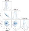 |
Fig. 2. Constraints on the dark-matter density profile of Eridanus 2 in the astrophysical parametrization, assuming CDM, found using CJAM and MultiNest. Units are omitted for clarity. The parameters are the characteristic dark-matter density (ρ0) in M⊙ kpc−3, the scale radius (rs) in kpc, and the systemic velocity (v0) in km s−1. The contours correspond to 0.5σ, 1.0σ, 1.5σ, and 2.0σ confidence levels, where σ is the standard deviation of a two-dimensional normal distribution. The vertical dashed lines in the one-dimensional histograms indicate the median and the 68% confidence interval. |
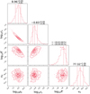 |
Fig. 3. Constraints on the dark-matter density profile of Eridanus 2 in the microphysical parametrization, assuming SIDM, found using CJAM and MultiNest. Units are omitted for clarity. The parameters are the characteristic dark-matter density (ρ0) in M⊙ kpc−3, the scale radius (rs) in kpc, the effective self-interaction coefficient (fΓ) in cm3 s−1 eV−1 c2, and the systemic velocity (v0) in km s−1. The contours correspond to 0.5σ, 1.0σ, 1.5σ, and 2.0σ confidence levels, where σ is the standard deviation of a two-dimensional normal distribution. The vertical dashed lines in the one-dimensional histograms indicate the median and the 68% confidence interval (without arrows) or the 68% and 95% confidence limits (upper and lower arrows, respectively). |
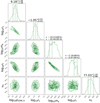 |
Fig. 4. Constraints on the dark-matter density profile of Eridanus 2 in the microphysical parametrization, assuming FDM, found using CJAM and MultiNest. Units are omitted for clarity. The parameters are the characteristic dark-matter density of the CDM-like outer profile (ρCDM, 0) in M⊙ kpc−3, the scale radius (rs) of the CDM-like outer profile in kpc, the dark-matter particle mass (ma) in eV c−2, the transition radius (rt) between the inner soliton and outer CDM-like profile in kpc, and the systemic velocity (v0) in km s−1. The contours correspond to 0.5σ, 1.0σ, 1.5σ, and 2.0σ confidence levels, where σ is the standard deviation of a two-dimensional normal distribution. The vertical dashed lines in the one-dimensional histograms indicate the median and the 68% confidence interval (without arrows) or the 68% and 95% confidence limits (upper and lower arrows, respectively). |
CJAM ρ0and rs. For the CDM profile we find a characteristic density of  and a scale radius of
  . The SIDM profile has consistent values for the same parameters:
  and
and  . This indicates that at large radii the density profiles of CDM and SIDM are in agreement.
CJAM SIDM rcand fΓ. Considering that the SIDM core radius is consistent with a scale radius smaller than our smallest projected radius (1.96 pc), we lack constraining power at the lower end of the range of this parameter. It is therefore appropriate to present the constraint as an upper limit: rc/pc < 101.67 = 47 at the 68% confidence level and rc/pc < 102.07 = 117 at the 95% confidence level. For the related effective self-interaction coefficient, we find that fΓ/(cm3 s−1 eV−1 c2) < 10−28.65 = 2.2 × 10⁻²⁹ at the 68% confidence level and fΓ/(cm3 s−1 eV−1 c2) < 10−28.09 = 8.1 × 10⁻²⁹ at the 95% confidence level.
CJAM FDM rsol and ma. In the case of the FDM model, it is also appropriate to present the soliton radius as an upper limit: rsol/pc < 100.86 = 7.2 at the 68% confidence level and rsol/pc < 102.01 = 102 at the 95% confidence level. Because of the degeneracy between the soliton radius and central soliton density, the central soliton density should be understood as a lower limit: ρsol, 0/(M⊙ kpc−3) > 1011.89 = 7.8 × 10¹¹ at the 68% confidence level and ρsol, 0/(M⊙ kpc−3) > 1010.13 = 1.3 × 10¹⁰ at the 95% confidence level. The equivalent dark-matter particle mass is given as ma/(eV c−2) > 10−19.23 = 5.9 × 10⁻²⁰ at the 68% confidence level and ma/(eV c−2) > 10−20.40 = 4.0 × 10⁻²¹ at the 95% confidence level.
pyGravSphere. Figures 5–7 show the parameter constraints for the pyGravSphere NFW, Hernquist–Zhao, and broken power-law models, respectively. The characteristic density of the NFW model is  and its scale radius is
  , which is consistent with the CJAM CDM results but is also strongly degenerate. For the Hernquist–Zhao model, we find that
  and
and  , which is again consistent but degenerate. The characteristic density of the broken power-law model,
  , is not directly comparable to the other characteristic densities due to the difference in the definitions, but it is notable that this parameter is much better constrained. The Hernquist–Zhao model prefers inner slopes γ > 0.57 at the 68% confidence level and γ > 0.10 at the 95% confidence level that are consistent with a cusp, while the broken power-law model has a weak preference for a core with γ0 < 1.47 at the 68% confidence level and γ0 < 2.51 at the 95% confidence level, but also still consistent with a cusp. Conversely, the Hernquist–Zhao model weakly prefers outer slopes consistent with CDM, with β < 6.99 at the 68% confidence level and β < 8.68 at the 95% confidence level, while the broken power-law model prefers steeper slopes with γ4 > 7.00 at the 68% confidence level and γ4 > 4.74 at the 95% confidence level. The shape of the Hernquist–Zhao profile is thus consistent with the NFW profile, albeit with large uncertainty, while the shape of the broken power-law profile deviates at large radii by over 2σ. The constraints on the velocity anisotropies are in general very weak, with an apparent trend for positive (radial) anisotropy in the case of the Hernquist–Zhao profile and for the centre in the case of the NFW profile. At large radii the NFW profile seems to prefer isotropy. The broken power-law model profile, on the other hand, prefers isotropy for the centre and negative (tangential) anisotropy for the outer radii. The transition between these possibly different regimes of inner and outer velocity anisotropy is essentially unconstrained.
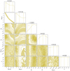 |
Fig. 5. Constraints on the dark-matter density profile of Eridanus 2, assuming an NFW profile, found using pyGravSphere. Units are omitted for clarity. The parameters are the characteristic dark-matter density (ρ0) in M⊙ kpc−3, the scale radius (rs) in kpc, the symmetrized inner and outer velocity anisotropy ( |


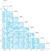 |
Fig. 6. Constraints on the dark-matter density profile of Eridanus 2, assuming a Hernquist–Zhao profile, found using pyGravSphere. Units are omitted for clarity. The parameters are the characteristic dark-matter density (ρ0) in M⊙ kpc−3, the scale radius (rs) in kpc, the inner and outer negative logarithmic slopes (γ and β) and the sharpness (α) of their transition, the symmetrized inner and outer velocity anisotropy ( |


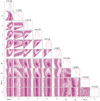 |
Fig. 7. Constraints on the dark-matter density profile of Eridanus 2, assuming a broken power-law profile, found using pyGravSphere. Units are omitted for clarity. The parameters are the characteristic dark-matter density (ρ0) in M⊙ kpc−3, the negative power-law slopes (γ0, …, γ4), the symmetrized inner and outer velocity anisotropy ( |


3.2. Profile recovery
The two methods that we use to constrain the density profile of Eri 2, CJAM and pyGravSphere, have one profile model in common: the CDM (NFW) profile. By comparing the constraints on this profile model obtained with the two methods, we can gauge the influence of the different assumptions that go into the methods. In Fig. 8 we show the recovered CDM (NFW) density profiles as a function of radius in the form of the median density and the 68% confidence interval at every radius. Although there are differences, most noticeably that pyGravSphere prefers lower central densities and higher outer densities than CJAM, the overall agreement is good. The two recovered profiles agree within the uncertainties at every radius, and there is no systematic preference for higher or lower densities. This indicates that the different assumptions have no significant effect on the recovered constraints and lends support to the results of both methods.
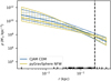 |
Fig. 8. Recovered dark-matter density profile of Eridanus 2, comparing the CJAM model for CDM with the pyGravSphere NFW profile. These models have the same functional form for the density profile but use different assumptions and methods of calculation. The hatched bands represent the 68% confidence interval on the density at each radius. The half-light radius is indicated with the vertical dashed line. The black markers at the bottom of the figure show the projected radii of the kinematic tracers. Tracers in bins rejected by pyGravSphere are marked in grey. |
The recovered profiles using all models are displayed in Fig. 9. Around the radius where we have the largest number of tracers, the agreement between the profiles is the best and the uncertainties are the smallest. At larger radii, five of the models agree very well, but the broken power-law model prefers lower densities in its last bin. This lower density could be an indication of the effect of tidal truncation, but the data are insufficient to conclude this, as we will show below. The disagreement is the largest at small radii, where the density at the projected position of the innermost tracer varies from ∼109.5 M⊙ kpc−3 to ∼1011.5 M⊙ kpc−3. This is not surprising considering the lack of tracers at these radii and that by design some models have more freedom at small radii. All profiles are in agreement at the smaller radii, considering their uncertainties. In Appendix E we show the recovered intrinsic velocity dispersion profiles and compare them to estimates directly derived from the measured line-of-sight velocities.
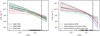 |
Fig. 9. Recovered dark-matter density profile of Eridanus 2. Left: CJAM models for CDM, SIDM, and FDM. Right: pyGravSphere models with NFW, Hernquist–Zhao, and broken power-law profiles. The hatched bands represent the 68% confidence interval on the density at each radius. The half-light radius is indicated with the vertical dashed line. The black markers at the bottom of the figure show the projected radii of the kinematic tracers. Tracers in bins rejected by pyGravSphere are marked in grey. |
We display the local mass-to-light ratio as a function of radius in Fig. 10. The density profile is divided by the V-band luminosity density profile, computed by de-projecting the exponential surface brightness profile from Crnojević et al. (2016) using the equation derived by Baes & Gentile (2011). This is a local, three-dimensional mass-to-light ratio at the indicated radius, not a cumulative mass-to-light ratio within that radius. Since the luminosity density profile is the same for every dark-matter model, the same differences are visible between the models. For most models the local mass-to-light radius has a minimum of  around the half-light radius.
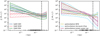 |
Fig. 10. Recovered de-projected mass-to-light profiles of Eridanus 2. These profiles show the local ratio of dark-matter density over luminosity density as a function of radius. The light profile is the exponential profile determined by Crnojević et al. (2016). Left: CJAM models for CDM, SIDM, and FDM. Right: pyGravSphere models with NFW, Hernquist–Zhao, and broken power-law dark-matter profiles. The hatched bands represent the 68% confidence interval on the mass-to-light ratio at each radius. The half-light radius is indicated with the vertical dashed line. The black markers at the bottom of the figure show the projected radii of the kinematic tracers. Tracers in bins rejected by pyGravSphere are marked in grey. |
We computed virial and half-light quantities as well as the maximum circular velocity from the density profiles and list them in Tables 4 and 5 for CJAM and pyGravSphere profiles, respectively. There is good agreement between the different profiles and between CJAM and pyGravSphere for the maximum circular velocity (Vmax) and for the mass within the projected half-light radius (M1/2), and as a consequence also for the integrated mass-to-light ratio, Υ1/2 = M1/2/(LV/2), within the same radius. The virial mass (M200) and the virial mass-to-light ratio (Υ200 = M200/LV) are more divergent from model to model. This is a consequence of the virial radius (r200) being an order of magnitude larger than the projected radius of the outermost tracer. For the calculation of the virial quantities, the density profiles were extrapolated to an extent that a small change in the profile slope around the outermost tracer leads to a large difference in the virial radius and virial mass. From the virial mass, the V-band luminosity, and the stellar mass-to-light ratio of 1.56 derived in Paper I, we can estimate a stellar-mass/halo-mass ratio of ∼10−3. For this value a galaxy is expected to reside in a halo that is intermediate between cuspy and cored (Di Cintio et al. 2014b).
Quantities derived from the CJAM-MultiNest density or mass profiles of Eridanus 2 under the assumptions of different profile models.
Quantities derived from the pyGravSphere-emcee density or mass profiles of Eridanus 2 under the assumptions of different profile models.
We also list in Tables 4 and 5 the astrophysical factors J and D, which are used to calculate the (gamma-ray) flux from annihilation and decay, respectively, of dark-matter particles (Bergström et al. 1998). They are integrals of the density profile or its square, over the line-of-sight (l) and a solid angle in the plane of the sky (ΔΩ):
We calculated these integrals up to the critical integration angle, which is the planar angle corresponding to the circular solid angle for which these factors are found to be most constrained for dwarf spheroidal galaxies. The critical integration angle is the angle subtended by the half-light radius for the D factor ( ) (Bonnivard et al. 2015b) and twice the half-light radius for the J factor (
 ) (Walker et al. 2011). The J and D factors are generally consistent within their uncertainties, though there is some tension for the D factor between the SIDM and broken power-law models.
3.3. Model comparison
We have so far placed constraints on astrophysical and microphysical parameters assuming different models and informally compared the different models based on the recovered profiles. The next question to ask is which model provides the best fit to the data, the answer to which may indicate a preference for one form of dark matter over another. In Tables 6 and 7 we present the Bayesian evidence (Z) for the CJAM and pyGravSphere models, respectively. The use of Bayesian evidence ensures that the different models employed with the same method can be fairly compared, taking into account that these models have different degrees of freedom. We assumed the prior probabilities of the models to be equal. Models were compared by taking the ratio of their Bayesian evidence (Z) or, equivalently, the difference between their log10(Z) values, with the model with the largest Z being favoured. The ratios or differences were interpreted using a scale; we used the scale from Jeffreys (1961, their Appendix B). According to this scale, a ratio of 100 or Δlog10(Z) = 2 is required for a decisive result. It is not possible to compare a model from one table to one from the other table because of the differences in the CJAM and pyGravSphere methods.
Bayesian evidence comparison for CJAM-MultiNest models.
Bayesian evidence comparison for pyGravSphere-emcee models using MCEvidence.
In all cases, the differences between the models are small. Among the CJAM models, the FDM profile has the largest Bayesian evidence. The Bayes factors indicate that the preference for FDM over SIDM is strong, but by no means significant, while FDM is only barely preferred over CDM. The preference for CDM over SIDM is substantial. It is therefore not possible to rule out any of the three dark-matter theories with the current data. For the pyGravSphere models, the broken power-law model is substantially preferred over the NFW model and the Hernquist–Zhao model. The modest strength of the evidence for the broken power-law model indicates that moving away from an NFW-like profile with a logarithmic slope of −3 at large radii is not required at present. Thus we find no conclusive evidence for tidal stripping or truncation at the probed radii. Further data at larger radii will help constrain the effect of tidal stripping.
4. Discussion
The mass–concentration relation between the virial mass (M200) and the concentration parameter c200 ≔ r200/rs from Dutton & Macciò (2014) predicts log10c200 ≈ 1.3 for an NFW halo with a virial mass equal to that of Eri 2 at redshift zero, with a scatter of 0.11 dex, but it was calibrated on a simulation with significantly higher virial masses (M200 ≳ 1012 h−1 M⊙). Using the semi-analytical relation of COMMAH (Correa et al. 2015a,b,c), we calculated a predicted concentration log10c200 ≈ 1.2. Our determinations of log10c200 for the CJAM models are more than one standard deviation higher. As M200 and c200 are among our less well-constrained parameters, we also performed a comparison in the space of two better constrained parameters for the CDM (NFW) profile of CJAM. Given the recovered rs, we predicted the density at 100 pc assuming the Dutton & Macciò (2014) mass–concentration relation,  . Compared to the recovered
  , this prediction is over two combined standard deviations lower, indicating that the tension between M200 and c200 is even larger than suggested at face value. Satellite dwarf galaxies are biased towards larger concentrations because higher-concentration dwarf galaxies are more likely to survive accretion by a Milky Way–mass galaxy (Nadler et al. 2018). This bias might explain (part of) the tension we see.
Using the stellar mass-to-halo mass relation of Behroozi et al. (2013) with the stellar mass-to-light ratio of 1.56 derived in Paper I, we expected a virial mass-to-light ratio  for Eri 2. Most of our models agree with this value, but there is a substantial tension for the SIDM and broken power-law models. Our half-light mass-to-light ratios (Υ1/2) are all consistent with the value
  found by Li et al. (2017).
The values that we find for the astrophysical factors are typical for dwarf spheroidal galaxies and UFDs (Bonnivard et al. 2015a; Alvarez et al. 2020). Eri 2 is therefore not the most interesting single target for observations concerning annihilation and decay signals, but it may be useful in a joint analysis of dwarf galaxies. Bonnivard et al. (2015b) have shown that the astrophysical factors can be biased by a factor of a few when an incorrect light profile model or halo triaxiality is assumed. We have assumed the light profile is exponential and the dark-matter halo is spherical, and therefore this bias may be present.
The self-interaction coefficient (Γ) can be described in terms of more conventional parameters by examining Eq. (2) and considering that the mass change is −2m per annihilation event, with m being the mass of the dark-matter particle. Assuming a cross-section σ and a typical velocity v, we derive

Our constraints on the effective self-interaction coefficients therefore translate to σ/m< 1.1 ×10−36 (f/10)−1(v/10 km s−1)−1 cm2 eV−1 c2 at the 68% confidence level and σ/m< 4.1 ×10−36 (f/10)−1(v/10 km s−1)−1 cm2 eV−1 c2 at the 95% confidence level, where f = 10 and v = 10 km s−1 are of the right order of magnitude for UFDs. Much stronger constraints exist from combined observations of dwarf galaxies with the Fermi/LAT and MAGIC gamma-ray telescopes (MAGIC collaboration 2016), equivalent to upper limits as low as ∼10−43 (v/10 km s−1) cm2 eV−1 c2. These constraints, however, are only valid for 101 GeV c−2 ≤ m ≤ 105 GeV c−2 and depend on the annihilation products, while our constraint is valid for all masses and annihilation products. The results from density profiles and gamma-ray searches are therefore complementary.
Lin & Loeb (2016) remarked that Γ can also represent self-interaction through scattering. Dark-matter particles can be scattered from the dense inner regions, where interactions are most likely, to the outer regions, where their contribution to the local density is negligible due to the much larger area. This is effectively equivalent to an annihilation of dark-matter particles, but the strength of the effect depends on how frequent a scattering event leads to particles leaving the centre of the dark-matter halo. This frequency is currently unknown; therefore, it is not possible to convert Γ to a scattering cross-section. Other profiles for SIDM that are designed specifically for a scattering self-interaction exist, such as the profiles of Kaplinghat et al. (2014, 2016), but these are outside the scope of this paper. Hayashi et al. (2021) used the latter profile on 23 UFDs using literature kinematics and found no evidence for a non-zero self-interaction in these galaxies.
Our lower limit on the FDM-particle mass of ma > 4.0 × 10⁻²¹ eV c−2 at the 95% confidence level is incompatible with some results for other dwarf galaxies. Chen et al. (2017) find  or
or  , depending on the dataset used, for the eight classical dwarf spheroidal galaxies. For the ultra-diffuse galaxy Dragonfly 44, Wasserman et al. (2019) find
  . Broadhurst et al. (2020) find
  for the ultra-diffuse galaxy Antlia II and ma = 1.07 ± 0.08 × 10⁻²² eV c−2 when combined with four classical dwarf spheroidal galaxies. This discrepancy might indicate that the cores in the literature galaxies, which have higher masses than Eri 2, are formed by baryonic processes (Brooks & Zolotov 2014; Di Cintio et al. 2014a) and not (entirely) by FDM. Other constraints on FDM from Eri 2 have been derived from the survival of its star cluster (Marsh & Niemeyer 2019; El-Zant et al. 2020). These constraints rule out at least the mass range between ∼10−20 eV c−2 and ∼10−19 eV c−2 and can likely be extended further, with some caveats.
In simulations of spherically symmetric and relaxed FDM haloes, a scaling relation between the size of the soliton, the mass of the FDM particle, and the virial mass of the halo is found at redshift zero (Schive et al. 2014b; Nori & Baldi 2021):
where rc = (9.1 × 10⁻²)1/2rsol and m22 = ma/(10−22 eV c−2). From the perspective of a single halo, m22rc is a constant. We find  directly from ma and rsol, which is consistent with the expected
  based on the virial mass of Eri 2.
Amorisco (2017) and Contenta et al. (2018) argue that the survival and projected location of the star cluster in Eri 2 imply that Eri 2 has a cored density profile. If the inner slope of the density profile is larger than ∼0.2–0.25, a cluster in a tight orbit would be tidally destroyed, while it would be unlikely to observe a cluster in a wide orbit so close in projection to the centre of Eri 2. The cluster could survive if it is stationary at the centre of the dark-matter halo of Eri 2, but that would mean that the photometric and gravitational centres of Eri 2 do not coincide. Our estimates of the inner slope are inconclusive in this respect: On the one hand, the broken power-law profile prefers a core, while on the other, the Hernquist–Zhao profile disagrees by nearly 2σ.
We performed our pyGravSphere analysis with different numbers of stars per kinematic bin: 9 (the default of pyGravSphere for 92 stars in total), 11 (our fiducial analysis presented in this paper), 15, and 23. The recovered profiles for 11 and 15 stars per bin were consistent; we chose to use 11 stars per bin as this results in more bins and could therefore potentially better capture the behaviour at small radii. The pyGravSphere profiles for 9 stars per bin had a much larger scale radius and lower characteristic density, inconsistent with both the 11 and 15 bin profiles and the CJAM profiles. Binning the stars by 23 yielded only two bins with a positive intrinsic velocity dispersion, which is too few for pyGravSphere to run. Therefore, as far as we can test, the profiles recovered by pyGravSphere seem stable with respect to the number of stars per bin, as long as a minimum number of stars per bin is met. We meet this requirement for our fiducial analysis with 11 stars per bin.
Dynamical mass estimates are only correct if the system is in dynamical equilibrium. As we argued in Paper I, given that Eri 2 is currently close to its pericentre (Fritz et al. 2018), yet still 366 kpc removed from us (Crnojević et al. 2016), it has not closely approached the Milky Way. Nor have any tidal features been detected in deep imaging (Crnojević et al. 2016). Furthermore, the stars in Eri 2 are dominated by an old population (Simon et al. 2021). Therefore, we do not expect a significant departure from dynamical equilibrium due to either tidal interactions with the Milky Way or stellar feedback.
Another issue that can affect dynamical mass estimates is the presence of binary stars. Due to its orbital motion, the line-of-sight velocity of a binary star can change over time. Instead of the systemic velocity of the binary system, one sees another contribution on top of that, which may inflate measurements of velocity dispersion. We have observed our fields at multiple epochs for over a year. By combining the exposures before the data reduction, the velocity variation of short-period binary stars is blended into broadened spectral features. These should have the same centroid as the binary-systemic line-of-sight velocities and should therefore not impact our measurements. Longer-period binary systems typically have lower line-of-sight velocity deviations, so they are not expected to be a significant problem. Nevertheless, there remains much to be studied regarding the binary-star populations of UFDs.
We have assumed that the dark-matter halo of Eri 2 is spherical even though the stellar distribution is not. This could potentially bias the dark-matter density profiles. Read & Steger (2017) have shown that GravSphere can become slightly biased for triaxial haloes, but the bias on the density profile is within the 95% confidence interval in most cases, as is the mass within the half-light radius. This test was done with mock data resembling classical dwarf galaxies; as we have less data and larger measurement uncertainties, we expected any bias on the pyGravSphere density profiles due to triaxiality to be even smaller relative to the confidence intervals than for the mock classical dwarfs. As we obtained similar results with CJAM and pyGravSphere, the CJAM density profiles should also not be significantly biased.
There is some uncertainty regarding the position of the centre of Eri 2. Mis-centring the spatial coordinates can affect the derived density profile because the density measured at the centre of the coordinate system will be lower than the density at the true centre of the galaxy. This effect can lead to cored density profiles being measured for cuspy dark-matter haloes, or to core radii being biased to larger values for cored haloes. We do not detect a core or soliton for Eri 2 and provide upper limits for the core and soliton radii. Our upper limits on core and soliton radii could therefore be biased high, but this would strengthen rather than weaken the confidence level of these limits.
5. Conclusions
We have presented new data from the MUSE-Faint survey of the UFD Eridanus 2 (MV = −7.1, M* ≈ 9 × 10⁴ M⊙). Ultra-faint dwarf galaxies have the lowest baryonic fractions of all known galaxies, and the baryonic contents are not believed to have altered the dark-matter density profiles. We have modelled the dark-matter density profile of Eridanus 2 using stellar kinematics from MUSE-Faint and from the literature (92 stars in total) to constrain the properties of SIDM and FDM and to compare these dark-matter models against one another and against CDM. For modelling the density profiles we have used both CJAM and pyGravSphere, two codes that use different methods and assumptions, to test whether the recovery of the density profile is sensitive to the approach that is used.
We constrained the core radius of the SIDM profile to rc < 47 pc (68% confidence level) or rc< 117 pc (95% confidence level). This translates into a constraint on the effective self-interaction coefficient of fΓ< 2.2 ×10⁻²⁹cm3s−1eV−1c2 (68% confidence level) or fΓ < 8.1 × 10⁻²⁹cm3s−1eV−1c2 (95% confidence level). These effective self-interaction coefficients are equivalent to the specific annihilation cross-sections σ/m< 1.1 ×10−36(f/10)−1(v/10 km s−1)−1 cm2 eV−1 c2 (68% confidence level) or σ/m < 4.1 × 10−36(f/10)−1(v/10 km s−1)−1 cm2 eV−1 c2 (95% confidence level). These constraints apply for all dark-matter particle masses and are therefore complementary to the results from gamma-ray searches for annihilation signatures, which provide stronger constraints in a limited mass range.
We constrained the soliton radius of the FDM profile to rsol < 7.2 pc (68% confidence level) or rsol < 102 pc (95% confidence level). The equivalent constraint on the mass of the ultra-light dark-matter particle is ma > 5.9×−20 eV c−2 (68% confidence level) or ma > 4.0 × 10⁻²¹ eV c−2 (95% confidence level). These constraints are inconsistent with particle masses for larger dwarf galaxies, which may indicate that the cores in these larger dwarf galaxies are not caused by FDM.
We could not consistently constrain the velocity anisotropy of Eridanus 2. CJAM and pyGravSphere prefer different values for the inner and outer slope of the density profile when these are free parameters of the profile; therefore, we cannot draw conclusions about the survival or location of the star cluster.
We found that CJAM and pyGravSphere recover similar dark-matter density profiles for Eridanus 2 when a CDM-NFW profile is assumed in both cases. All CJAM and pyGravSphere profiles are consistent within their uncertainties. The uncertainty on the profile and the difference between the profiles become larger near the centre of Eridanus 2, where the kinematic data are sparse.
From the dark-matter density profiles we determined virial masses M200 ∼ 108 M⊙, maximum circular velocities Vmax ∼ 101.2–101.4 km s−1, half-light mass-to-light ratios Υ1/2 ∼ 102.5 M⊙  and astrophysical factors
  and
and  –102.5 M⊙ kpc−2. The half-light mass-to-light ratio is consistent with the literature, and the astrophysical factors are typical for dwarf galaxies. For CJAM with the CDM model, the values are
  ,
,  , Υ1/2 =
  ,
,  , and
, and 
 . The concentration c ∼ 101.5–102 (
 for CJAM with CDM) is for several profiles higher than the expected value for a galaxy of this virial mass, but this may be because Eridanus 2 is a satellite of the Milky Way.
We found a weak preference for FDM over CDM and substantial evidence for CDM over SIDM. The evidence to prefer FDM over SIDM is strong. This indicates a preference for a cusp over a core, but also for a soliton over a cusp. None of the models are preferred decisively over any other, and therefore it is not possible to rule out CDM, SIDM, or FDM.
With MUSE-Faint we have been able to significantly increase the number of stars with spectroscopy inside the half-light radius of Eridanus 2 and have extended the available data to smaller radii. Nevertheless, it remains challenging to obtain a large sample of stellar line-of-sight velocities in such a faint and distant system. Improvements of the constraints on the inner dark-matter density profile of Eridanus 2 and its implications for the nature and properties of dark matter would require deeper observations or observations at a higher spectral resolution. Deeper observations could improve the line-of-sight velocity measurements and could provide access to fainter stars but would be a costly undertaking. A higher spectral resolution could significantly decrease the velocity uncertainties, but current high-resolution spectrographs are not able to reach the spatial resolution required for these crowded systems. It would also be valuable to extend the current study to multiple UFDs and test whether our conclusions also hold for other systems.
Hubble Space Telescope proposal GO-14234, principal investigator J. D. Simon, presented by Simon et al. (2021).
Acknowledgments
We thank the anonymous referee for their helpful comments, which improved the manuscript. SLZ wishes to thank Anna Genina and Justin I. Read for interesting and useful discussions, and Mariana P. Júlio for asking helpful questions. SLZ acknowledges support by The Netherlands Organisation for Scientific Research (NWO) through a TOP Grant Module 1 under project number 614.001.652. JB acnowledges support by Fundação para a Ciência e a Tecnologia (FCT) through the research grants UID/FIS/04434/2019, UIDB/04434/2020, UIDP/04434/2020 and through the Investigador FCT Contract No. IF/01654/2014/CP1215/CT0003. Based on observations made with ESO Telescopes at the La Silla Paranal Observatory under programme IDs 0100.D-0807, 0102.D-0372, 0103.D-0705, and 0104.D-0199. This research has made use of Astropy (Astropy Collaboration 2013, 2018), corner.py (Foreman-Mackey 2016), matplotlib (Hunter 2007), NASA’s Astrophysics Data System Bibliographic Services, NumPy (Harris et al. 2020), SciPy (Virtanen et al. 2020), and the colour schemes of Tol (2018). This work has made use of data from the European Space Agency (ESA) mission Gaia (https://www.cosmos.esa.int/web/gaia), processed by the Gaia Data Processing and Analysis Consortium (DPAC, https://www.cosmos.esa.int/web/gaia/dpac/consortium). Funding for the DPAC has been provided by national institutions, in particular the institutions participating in the Gaia Multilateral Agreement. This research made use of Montage. It is funded by the National Science Foundation under Grant Number ACI-1440620, and was previously funded by the National Aeronautics and Space Administration’s Earth Science Technology Office, Computation Technologies Project, under Cooperative Agreement Number NCC5-626 between NASA and the California Institute of Technology.
References
- Alvarez, A., Calore, F., Genina, A., et al. 2020, JCAP, 2020, 004 [CrossRef] [Google Scholar]
- Amorisco, N. C. 2017, ApJ, 844, 64 [CrossRef] [Google Scholar]
- Amorisco, N. C., Agnello, A., & Evans, N. W. 2013, MNRAS, 429, L89 [CrossRef] [Google Scholar]
- Astropy Collaboration (Robitaille, T. P., et al.) 2013, A&A, 558, A33 [NASA ADS] [CrossRef] [EDP Sciences] [Google Scholar]
- Astropy Collaboration (Price-Whelan, A. M., et al.) 2018, AJ, 156, 123 [Google Scholar]
- Bacon, R., Accardo, M., Adjali, L., et al. 2010, Proc. SPIE, 7735, 773508 [Google Scholar]
- Bacon, R., Conseil, S., Mary, D., et al. 2017, A&A, 608, A1 [NASA ADS] [CrossRef] [EDP Sciences] [Google Scholar]
- Baes, M., & Gentile, G. 2011, A&A, 525, A136 [NASA ADS] [CrossRef] [EDP Sciences] [Google Scholar]
- Baes, M., & Van Hese, E. 2007, A&A, 471, 419 [NASA ADS] [CrossRef] [EDP Sciences] [Google Scholar]
- Battaglia, G., Helmi, A., Tolstoy, E., et al. 2008, ApJ, 681, L13 [NASA ADS] [CrossRef] [Google Scholar]
- Behroozi, P. S., Wechsler, R. H., & Conroy, C. 2013, ApJ, 770, 57 [Google Scholar]
- Bergström, L., Ullio, P., & Buckley, J. H. 1998, Astropart. Phys., 9, 137 [NASA ADS] [CrossRef] [MathSciNet] [Google Scholar]
- Bonnivard, V., Combet, C., Daniel, M., et al. 2015a, MNRAS, 453, 849 [CrossRef] [Google Scholar]
- Bonnivard, V., Combet, C., Maurin, D., & Walker, M. G. 2015b, MNRAS, 446, 3002 [CrossRef] [Google Scholar]
- Breddels, M. A., Helmi, A., van den Bosch, R. C. E., van de Ven, G., & Battaglia, G. 2013, MNRAS, 433, 3173 [NASA ADS] [CrossRef] [Google Scholar]
- Broadhurst, T., De Martino, I., Luu, H. N., Smoot, G. F., & Tye, S. H. H. 2020, Phys. Rev. D, 101, 083012 [CrossRef] [Google Scholar]
- Brooks, A. M., & Zolotov, A. 2014, ApJ, 786, 87 [NASA ADS] [CrossRef] [Google Scholar]
- Buchner, J., Georgakakis, A., Nandra, K., et al. 2014, A&A, 564, A125 [NASA ADS] [CrossRef] [EDP Sciences] [Google Scholar]
- Cappellari, M. 2008, MNRAS, 390, 71 [NASA ADS] [CrossRef] [Google Scholar]
- Carlson, E. D., Machacek, M. E., & Hall, L. J. 1992, ApJ, 398, 43 [CrossRef] [Google Scholar]
- Chen, S.-R., Schive, H.-Y., & Chiueh, T. 2017, MNRAS, 468, 1338 [NASA ADS] [CrossRef] [Google Scholar]
- Choi, J., Dotter, A., Conroy, C., et al. 2016, ApJ, 823, 102 [Google Scholar]
- Contenta, F., Balbinot, E., Petts, J. A., et al. 2018, MNRAS, 476, 3124 [NASA ADS] [CrossRef] [Google Scholar]
- Correa, C. A., Wyithe, J. S. B., Schaye, J., & Duffy, A. R. 2015a, MNRAS, 450, 1514 [NASA ADS] [CrossRef] [Google Scholar]
- Correa, C. A., Wyithe, J. S. B., Schaye, J., & Duffy, A. R. 2015b, MNRAS, 450, 1521 [NASA ADS] [CrossRef] [Google Scholar]
- Correa, C. A., Wyithe, J. S. B., Schaye, J., & Duffy, A. R. 2015c, MNRAS, 452, 1217 [NASA ADS] [CrossRef] [Google Scholar]
- Crnojević, D., Sand, D. J., Zaritsky, D., et al. 2016, ApJ, 824, L14 [NASA ADS] [CrossRef] [Google Scholar]
- Di Cintio, A., Brook, C. B., Macciò, A. V., et al. 2014a, MNRAS, 437, 415 [Google Scholar]
- Di Cintio, A., Brook, C. B., Dutton, A. A., et al. 2014b, MNRAS, 441, 2986 [Google Scholar]
- Dodelson, S., & Widrow, L. M. 1994, Phys. Rev. Lett., 72, 17 [NASA ADS] [CrossRef] [PubMed] [Google Scholar]
- Dotter, A. 2016, ApJS, 222, 8 [NASA ADS] [CrossRef] [Google Scholar]
- Dutton, A. A., & Macciò, A. V. 2014, MNRAS, 441, 3359 [Google Scholar]
- Dwyer, P. S. 1937, Ann. Math. Stat., 8, 21 [CrossRef] [Google Scholar]
- El-Zant, A. A., Freundlich, J., & Combes, F. 2016, MNRAS, 461, 1745 [Google Scholar]
- El-Zant, A. A., Freundlich, J., Combes, F., & Halle, A. 2020, MNRAS, 492, 877 [CrossRef] [Google Scholar]
- Emsellem, E., Monnet, G., & Bacon, R. 1994, A&A, 285, 723 [NASA ADS] [Google Scholar]
- Fermi-LAT Collaboration 2014, Phys. Rev. D, 89, 042001 [NASA ADS] [CrossRef] [Google Scholar]
- Feroz, F., & Hobson, M. P. 2008, MNRAS, 384, 449 [NASA ADS] [CrossRef] [Google Scholar]
- Feroz, F., Hobson, M. P., & Bridges, M. 2009, MNRAS, 398, 1601 [NASA ADS] [CrossRef] [Google Scholar]
- Feroz, F., Hobson, M. P., Cameron, E., & Pettitt, A. N. 2019, Open J. Astrophys., 2, 10 [Google Scholar]
- Ferreira, E. G. M. 2020, A&ARv, in press [arXiv:2005.03254] [Google Scholar]
- Fisher, R. A. 1930, Proc. Lond. Math. Soc., 30, 199 [CrossRef] [Google Scholar]
- Foreman-Mackey, D. 2016, J. Open Source Softw., 1, 24 [Google Scholar]
- Foreman-Mackey, D., Hogg, D. W., Lang, D., & Goodman, J. 2013, PASP, 125, 306 [Google Scholar]
- Freundlich, J., Dekel, A., Jiang, F. Z., et al. 2020, MNRAS, 491, 4523 [CrossRef] [Google Scholar]
- Fritz, T. K., Bahaglia, G., Pawlowski, M. S., et al. 2018, A&A, 619, A103 [NASA ADS] [CrossRef] [EDP Sciences] [Google Scholar]
- Gaia Collaboration (Prusti, T., et al.) 2016, A&A, 595, A1 [NASA ADS] [CrossRef] [EDP Sciences] [Google Scholar]
- Gaia Collaboration (Brown, A. G. A., et al.) 2018, A&A, 616, A1 [NASA ADS] [CrossRef] [EDP Sciences] [Google Scholar]
- Genina, A., Read, J. I., Fattahi, A., & Frenk, C. S. 2020a, MNRAS, submitted [arXiv:2011.09482] [Google Scholar]
- Genina, A., Read, J. I., Frenk, C. S., et al. 2020b, MNRAS, 498, 144 [CrossRef] [Google Scholar]
- Goerdt, T., Moore, B., Read, J. I., Stadel, J., & Zemp, M. 2006, MNRAS, 368, 1073 [NASA ADS] [CrossRef] [Google Scholar]
- Griest, K. 1991, ApJ, 366, 412 [NASA ADS] [CrossRef] [Google Scholar]
- Harris, C. R., Millman, K. J., van der Walt, S. J., et al. 2020, Nature, 585, 357 [CrossRef] [PubMed] [Google Scholar]
- Hayashi, K., Ibe, M., Kobayashi, S., Nakayama, Y., & Shirai, S. 2021, Phys. Rev. D, 103, 023017 [CrossRef] [Google Scholar]
- Heavens, A., Fantaye, Y., Mootoovaloo, A., et al. 2017, ArXiv e-prints [arXiv:1704.03472] [Google Scholar]
- Hernquist, L. 1990, ApJ, 356, 359 [Google Scholar]
- Hu, W., Barkana, R., & Gruzinov, A. 2000, Phys. Rev. Lett., 85, 1158 [Google Scholar]
- Hunter, J. D. 2007, Comput. Sci. Eng., 9, 90 [NASA ADS] [CrossRef] [Google Scholar]
- Husser, T.-O. 2012, 3D-Spectroscopy of Dense Stellar Populations (Göttingen, Germany: Universitätsverlag Göttingen) [CrossRef] [Google Scholar]
- Jardel, J. R., Gebhardt, K., Fabricius, M. H., Drory, N., & Williams, M. J. 2013, ApJ, 763, 91 [NASA ADS] [CrossRef] [Google Scholar]
- Jeffreys, H. 1961, Theory of Probability, 3rd edn. (Oxford, United Kingdom: Clarendon) [Google Scholar]
- Kamann, S., Wisotzki, L., & Roth, M. M. 2013, A&A, 549, A71 [NASA ADS] [CrossRef] [EDP Sciences] [Google Scholar]
- Kaplinghat, M., Knox, L., & Turner, M. S. 2000, Phys. Rev. Lett., 85, 3335 [NASA ADS] [CrossRef] [Google Scholar]
- Kaplinghat, M., Keeley, R. E., Linden, T., & Yu, H. B. 2014, Phys. Rev. Lett., 113, 021302 [CrossRef] [Google Scholar]
- Kaplinghat, M., Tulin, S., & Yu, H.-B. 2016, Phys. Rev. Lett., 116, 041302 [CrossRef] [Google Scholar]
- Kleyna, J. T., Wilkinson, M. I., Evans, N. W., & Gilmore, G. 2005, ApJ, 630, L141 [NASA ADS] [CrossRef] [Google Scholar]
- Lazar, A., Bullock, J. S., Boylan-Kolchin, M., et al. 2020, MNRAS, 497, 2393 [CrossRef] [Google Scholar]
- Li, T. S., Simon, J. D., Drlica-Wagner, A., et al. 2017, ApJ, 838, 8 [NASA ADS] [CrossRef] [Google Scholar]
- Lin, H. W., & Loeb, A. 2016, JCAP, 03, 009 [CrossRef] [Google Scholar]
- Lindegren, L., Hernández, J., Bombrun, A., et al. 2018, A&A, 616, A2 [NASA ADS] [CrossRef] [EDP Sciences] [Google Scholar]
- Lupton, R., Blanton, M. R., Fekete, G., et al. 2004, PASP, 116, 133 [NASA ADS] [CrossRef] [Google Scholar]
- MAGIC collaboration (Ahnen, M. L., et al.) 2016, JCAP, 02, 039 [Google Scholar]
- Marsh, D. J. E., & Niemeyer, J. C. 2019, Phys. Rev. Lett., 123, 051103 [NASA ADS] [CrossRef] [Google Scholar]
- Marsh, D. J. E., & Pop, A.-R. 2015, MNRAS, 451, 2479 [NASA ADS] [CrossRef] [Google Scholar]
- Massari, D., Breddels, M. A., Helmi, A., et al. 2018, Nat. Astron., 2, 156 [NASA ADS] [CrossRef] [Google Scholar]
- Massari, D., Helmi, A., Mucciarelli, A., et al. 2020, A&A, 633, A36 [CrossRef] [EDP Sciences] [Google Scholar]
- McConnachie, A. W. 2012, AJ, 144, 4 [Google Scholar]
- Merrifield, M. R., & Kent, S. M. 1990, AJ, 99, 1548 [NASA ADS] [CrossRef] [Google Scholar]
- Milgrom, M. 1983, ApJ, 270, 365 [NASA ADS] [CrossRef] [Google Scholar]
- Nadler, E. O., Mao, Y.-Y., Wechsler, R. H., Garrison-Kimmel, S., & Wetzel, A. 2018, ApJ, 859, 129 [CrossRef] [Google Scholar]
- Navarro, J. F., Frenk, C. S., & White, S. D. M. 1996, ApJ, 462, 563 [Google Scholar]
- Nori, M., & Baldi, M. 2021, MNRAS, 501, 1539 [Google Scholar]
- Oman, K. A., Marasco, A., Navarro, J. F., et al. 2019, MNRAS, 482, 821 [NASA ADS] [CrossRef] [Google Scholar]
- Oñorbe, J., Boylan-Kolchin, M., Bullock, J. S., et al. 2015, MNRAS, 454, 2092 [NASA ADS] [CrossRef] [Google Scholar]
- Paxton, B., Bildsten, L., Dotter, A., et al. 2011, ApJS, 192, 3 [Google Scholar]
- Paxton, B., Cantiello, M., Arras, P., et al. 2013, ApJS, 208, 4 [NASA ADS] [CrossRef] [Google Scholar]
- Paxton, B., Marchant, P., Schwab, J., et al. 2015, ApJS, 220, 15 [Google Scholar]
- Peñarrubia, J., Pontzen, A., Walker, M. G., & Koposov, S. E. 2012, ApJ, 759, L42 [NASA ADS] [CrossRef] [Google Scholar]
- Plummer, H. C. 1911, MNRAS, 71, 460 [CrossRef] [Google Scholar]
- Preskill, J., Wise, M. B., & Wilczek, F. 1983, Phys. Lett. B, 120, 127 [NASA ADS] [CrossRef] [Google Scholar]
- Read, J. I., & Steger, P. 2017, MNRAS, 471, 4541 [NASA ADS] [CrossRef] [Google Scholar]
- Read, J. I., Wilkinson, M. I., Evans, N. W., Gilmore, G., & Kleyna, J. T. 2006, MNRAS, 367, 387 [NASA ADS] [CrossRef] [Google Scholar]
- Read, J. I., Agertz, O., & Collins, M. L. M. 2016, MNRAS, 459, 2573 [Google Scholar]
- Read, J. I., Walker, M. G., & Steger, P. 2018, MNRAS, 481, 860 [NASA ADS] [CrossRef] [Google Scholar]
- Read, J. I., Walker, M. G., & Steger, P. 2019, MNRAS, 484, 1401 [Google Scholar]
- Richardson, T., & Fairbairn, M. 2014, MNRAS, 441, 1584 [Google Scholar]
- Schive, H. Y., Chiueh, T., & Broadhurst, T. 2014a, Nat. Phys., 10, 496 [CrossRef] [Google Scholar]
- Schive, H. Y., Liao, M. H., Woo, T. P., et al. 2014b, Phys. Rev. Lett., 113 [Google Scholar]
- Simon, J. D. 2019, ARA&A, 57, 375 [NASA ADS] [CrossRef] [Google Scholar]
- Simon, J. D., Brown, T. M., Drlica-Wagner, A., et al. 2021, ApJ, 908, 18 [CrossRef] [Google Scholar]
- Soto, K. T., Lilly, S. J., Bacon, R., Richard, J., & Conseil, S. 2016, MNRAS, 458, 3210 [NASA ADS] [CrossRef] [Google Scholar]
- Spergel, D. N., & Steinhardt, P. J. 2000, Phys. Rev. Lett., 84, 3760 [Google Scholar]
- Steigman, G., & Turner, M. S. 1985, Nucl. Phys. B, 253, 375 [CrossRef] [Google Scholar]
- Strigari, L. E., Frenk, C. S., & White, S. D. M. 2018, ApJ, 860, 56 [NASA ADS] [CrossRef] [Google Scholar]
- Tol, P. 2018, Colour Schemes, Tech. Note SRON/EPS/TN/09-002, issue 3.1, SRON [Google Scholar]
- van de Ven, G., van den Bosch, R. C. E., Verolme, E. K., & de Zeeuw, P. T. 2006, A&A, 445, 513 [NASA ADS] [CrossRef] [EDP Sciences] [Google Scholar]
- Verlinde, E. 2017, SciPost Phys., 2, 016 [NASA ADS] [CrossRef] [Google Scholar]
- Virtanen, P., Gommers, R., Oliphant, T. E., et al. 2020, Nat. Methods, 17, 261 [Google Scholar]
- Walker, M. G., & Peñarrubia, J. 2011, ApJ, 742, 20 [NASA ADS] [CrossRef] [Google Scholar]
- Walker, M. G., Mateo, M., & Olszewski, E. W. 2009, AJ, 137, 3100 [NASA ADS] [CrossRef] [Google Scholar]
- Walker, M. G., Combet, C., Hinton, J. A., Maurin, D., & Wilkinson, M. I. 2011, ApJ, 733, L46 [NASA ADS] [CrossRef] [Google Scholar]
- Walker, M. G., Olszewski, E. W., & Mateo, M. 2015, MNRAS, 448, 2717 [NASA ADS] [CrossRef] [Google Scholar]
- Wasserman, A., van Dokkum, P., Romanowsky, A. J., et al. 2019, ApJ, 885, 155 [CrossRef] [Google Scholar]
- Watkins, L. L., van de Ven, G., den Brok, M., & van den Bosch, R. C. E. 2013, MNRAS, 436, 2598 [Google Scholar]
- Weilbacher, P. M., Palsa, R., Streicher, O., et al. 2020, A&A, 641, A28 [CrossRef] [EDP Sciences] [Google Scholar]
- Weinberg, S. 1978, Phys. Rev. Lett., 40, 223 [Google Scholar]
- Wheeler, C., Hopkins, P. F., Pace, A. B., et al. 2019, MNRAS, 490, 4447 [NASA ADS] [CrossRef] [Google Scholar]
- Wilczek, F. 1978, Phys. Rev. Lett., 40, 279 [NASA ADS] [CrossRef] [Google Scholar]
- Wolf, J., Martinez, G. D., Bullock, J. S., et al. 2010, MNRAS, 406, 1220 [NASA ADS] [Google Scholar]
- Zhao, H. S. 1996, MNRAS, 278, 488 [NASA ADS] [CrossRef] [Google Scholar]
- Zoutendijk, S. L., Brinchmann, J., Boogaard, L. A., et al. 2020, A&A, 635, A107 [CrossRef] [EDP Sciences] [Google Scholar]
Appendix A: Table of kinematics
In Table A.1 we list the positions and line-of-sight velocities of the stars used for the kinematic analysis in this paper.
Final selection of stars in Eridanus 2 for the kinematic analysis.
Appendix B: Multi-Gaussian expansions of the density profiles
The JAM method uses MGEs of the density profiles to speed up its calculations. The MGE itself is expensive, but for simple profiles it has to be computed only once. Some of our profiles, however, have parameters that modify their shape, which necessitates a different MGE for each combination of these parameter values. Because fitting the MGE separately for every Monte Carlo sample would be prohibitively expensive, we instead interpolated between MGEs fitted at a limited number of points in the parameter space. In this appendix we describe the fitting and interpolation procedures used to obtain the MGEs of our profiles.
For a scale-invariant profile such as the NFW profile, the MGE only needs to be done once, and the amplitude and standard deviations of the Gaussians can be rescaled to fit the NFW profile for any combination of characteristic density and scale radius. We performed the MGE on the NFW profile with 16 Gaussians by least-squares fitting at 64 logarithmically spaced points from 10−3 rs to 102 rs, weighting the residuals with the value of the NFW profile. The range of points chosen for fitting was deliberately broad in order to be sure that the observations were contained within the limits of this range for any reasonable choice of rs. In addition, the projection of the profile on the sky results in any radius larger than the projected radius being observed along the line of sight, and therefore the MGE needs to also reproduce the profile at radii larger than the largest projected radius. The resulting MGE is an accurate reproduction over the fitting range, with deviations in both the density and cumulative mass of the order of, at most, 1%.
The distribution of tracers was fitted with the same number of Gaussians to the exponential profile found by Crnojević et al. (2016), which has an effective radius of 2.31 arcmin and a central surface brightness of 27.2 mag. We also adopted their position angle of 72.6 deg and used their ellipticity ϵ = 0.48 to calculate a flattening of q = 1 − ϵ = 0.52. To reduce the computational complexity, we fixed the inclination to the default value of 90°, which corresponds to an edge-on system. The exponential drop-off is hard to reproduce over large orders of magnitude in radius, so we limited the fit to the range of 10−3 Re to 10 Re. A smaller range suffices here as we know the value of Re from photometry. The accuracy of the MGE is sub-percent over the fitting range for the density and for at least an extra magnitude of larger radii for the cumulative mass. The resulting fit is valid for all dark-matter models and does not need to be rescaled for different dark-matter parameters.
Unfortunately, a single MGE is not possible for the SIDM and FDM profiles. The computational expense of redoing the MGE for each combination of profile parameters is prohibitively large, and therefore we need to approximate the MGE with a faster method. For the SIDM profile, we performed the same procedure as for the NFW profile for 101 logarithmically spaced values of the core radius, from 10−2 rs to rs. We excluded models with a core radius larger than the NFW scale radius because such large cores are not expected given the existing work on dark-matter density profiles in dwarf galaxies (see e.g., the high-resolution simulations analysed by Lazar et al. 2020). The amplitudes and standard deviations of the 16 Gaussians vary smoothly with the core size, so we interpolated over these 101 results, supplemented with the NFW profile corresponding to a core size of zero, with quadratic splines. The 16 Gaussians returned by supplying the interpolator with a core radius can be rescaled with the characteristic density and scale radius, as for the NFW profile. We find that the resulting interpolated MGE is sufficiently close to a real MGE: The deviation from the original profile is still less than one percent. The interpolated MGE is also sufficiently fast for our purposes.
The FDM profile has the largest number of parameters of all our models and is therefore the most complex to expand into Gaussians. In addition to this, the profile proposed by Marsh & Pop (2015) has a sharp transition from the soliton part to the NFW part, which is very hard to approximate with a sum of Gaussians. Since this sharp transition was assumed for the sake of simplicity and the lack of detailed knowledge about the true transition, we find it justified to make a different simplifying assumption that suits our needs better. We approximated the FDM profile with the sum of a soliton and a cored NFW profile, the latter being the same profile that we used to model SIDM:

with  to ensure the characteristic density is correct. We find this to be a good approximation of ρFDM for a certain value of rc, depending on the values of the other parameters. Minimizing the difference between the two profiles at 64 logarithmically spaced points from 10−3 rsol to 102 rsol while varying rsol/rs over 101 logarithmically spaced values between 10−2 and 1, and ε over 101 logarithmically spaced values between 10−5 and 1/2, yields values of rc that roughly follow the relation
where C0 and C1 are constants. Enforcing this relation and repeating the minimization gives C0 ≈ 0.281 and C1 ≈ −0.0923. By construction, the profiles are identical at the centre and towards infinity. The largest deviation is at the transition radius; however, this is not a problem because it is very localized and because the original profile is only an approximation at this point. We then approximated the soliton profile with 16 Gaussians by fitting to 64 logarithmically spaced points from 10−3 rsol to 2rsol, at which point the soliton density has declined so far that it is negligible compared to the NFW part of the FDM profile. The soliton and SIDM fits were rescaled individually in accordance with the parameters of the profile, and they were then appended to form a MGE for the FDM profile. With this result we were able to approximate the original ρFDM with the MGE of  . At the transition radius the deviation can be very large, but elsewhere the accuracy is on the level of a few percent deviation from the original density profile.
Appendix C: Unbiased estimators of intrinsic velocity moments
With a small number of stars and relatively high uncertainties on their velocities, a careful estimation of the observed velocity moments and the correction term for measurement uncertainties is needed for a reliable dynamical analysis of UFDs. In this appendix we derive unbiased estimators of the second and fourth intrinsic velocity moments as well as an estimator of the uncertainty on the second intrinsic velocity moment. The estimators are exact when each velocity measurement has the same measurement uncertainty and are approximations when the measurement uncertainties are different.
Supposing we have N velocity measurements v1, v2, …, vN with measurement uncertainties ε1, ε2, …, εN, the velocities can be divided into bins with n measurements: vj + 1, vj + 2, …, vj + n. We assumed that the intrinsic – as opposed to observed – velocities in each bin are drawn from the same distribution and that the distributions of each bin have the same mean: the systemic velocity. Furthermore, we also assumed that the measurement errors are normally distributed around zero with a standard deviation equal to the measurement uncertainty. We were prevented from straightforwardly calculating the moments of the observed velocities by two effects: The measurement errors inflate the observed velocity moments, leading to a difference between the intrinsic and observed distributions, and the sample moments are biased estimators of the true moments of the observed distributions.
In the case of equal uncertainties on all measured velocities, the unbiased estimators of the intrinsic velocity moments can be determined exactly. For this we further assumed all measurement uncertainties to be equal to ε. We began by calculating the sample mean,

of all measurements as well as the rth sample central moments,
in each bin. The correction for the inflation of the moments by the measurement errors can be done using the cumulants because cumulants have the property

for random variables X and Y, in this case the intrinsic velocities and the measurement errors. The symmetrically unbiased estimators of the cumulants of a distribution are the k statistics (Fisher 1930), which for the second and fourth cumulants are
![$$ \begin{aligned}&k_4 = \frac{n^2 \Big [(n+1)m_4 - 3(n-1)m_2^2\Big ]}{(n-1)(n-2)(n-3)}\cdot \end{aligned} $$](/articles/aa/full_html/2021/07/aa40239-20/aa40239-20-eq138.gif)
The second and fourth cumulants of a normal distribution 𝒩(μ, σ2) are κ2 = σ2 and κ4 = 0. The distribution 𝒩(0, ε2) of measurement errors therefore has cumulants κ2, err = ε2 and κ4, err = 0. Correcting for the measurement uncertainty and using the properties of cumulants, the estimators of the intrinsic second and fourth cumulants are
Using Eqs. (C.4) and (C.5), this can be converted to the second and fourth intrinsic sample central moments:
The symmetrically unbiased estimators of the central moments of a distribution are given by the h statistics (Dwyer 1937). We can therefore estimate the intrinsic central moments in each bin with
![$$ \begin{aligned}&h_{4,\text{ int}} = \frac{n\Big [(n^2-2n+3)m_{4,\text{ int}} - 3(2n-3)m_{2,\text{ int}}^2\Big ]}{(n-1)(n-2)(n-3)}. \end{aligned} $$](/articles/aa/full_html/2021/07/aa40239-20/aa40239-20-eq144.gif)
In our case, where each velocity vi has its own uncertainty εi, there is no exact solution. Similar to van de Ven et al. (2006), we can try to approximate the correction of the cumulants with a single value. If the individual errors are interpreted as being drawn from a single distribution, the expected values of the second and fourth moments of this distribution are the averages of the same moments of the individual distributions: We supposed that the measurement errors are drawn from a single distribution and wanted to find the cumulants of this distribution. For an infinite number of draws, the sample raw moments converge to the true raw moments of a distribution:
If the draws from this supposed single distribution are equivalent to draws from n separate distributions of measurement errors, we can group draws from the same distribution together and write the above summation as
Comparing Eqs. (C.12) and (C.13), we can see that the latter equation is the average of the moments of the individual distributions. The central moments of the single distribution must therefore be
where we have used the assumption that the individual error distributions are normal distributions centred around zero,  , making the raw moments equal to the central moments. The cumulants to use as approximate correction terms in Eqs. (C.6) and (C.7) are therefore by definition

The correction for the second cumulant is the same as used by van de Ven et al. (2006).
There are two sources of uncertainty on the intrinsic moment estimators: measurement uncertainties and finite sampling. Both are reflected in the variance of the moments of the measured distribution. Remembering that the variance is the second raw moment of an estimator fr, we can write
![$$ \begin{aligned} \upmu _2(f_r) = {E}\Bigl [(f_r - {E}[f_r])^2\Bigr ] = \mathrm{E} \Bigl [(f_r)^2\Bigr ] - ({E}[f_r])^2 = \upmu \prime _2(f_r) - {\upmu \prime _1}^2(f_r), \end{aligned} $$](/articles/aa/full_html/2021/07/aa40239-20/aa40239-20-eq152.gif)
where E denotes the expectation value. From the equations and tables of Dwyer (1937), it follows that the variance of the second sample central moment is
Propagation of errors then gives us
In the right-hand side of this equation, μ2 and μ4 are the second and fourth true central moments of the observed velocity distribution. They are unknown, but we can approximate them with the h statistics:
Even though the h statistics are symmetrically unbiased estimators of the true central moments, the above approximation will have a bias because it is not a linear transformation. A further bias will be introduced by taking the square root to arrive at an estimate for the uncertainty:
In a similar way, we can estimate the uncertainty on the fourth intrinsic moment. This calculation depends, however, on even higher moments, up to the eighth. With the small number of stars per bin in this paper, it is not feasible to calculate this uncertainty to a good accuracy. As the VSPs depend on the fourth velocity moments, the uncertainty on the VSPs will also be challenging to constrain. We therefore opted not to use the VSPs in this paper.
Calculating the above estimators and uncertainty on mock data drawn from (i) known generalized normal distributions representing the intrinsic velocity distributions and (ii) normal distributions representing the measurement uncertainties (both of which are similar to the properties of the observed data) shows that the intrinsic moments and the uncertainty on the second moment can on average be recovered with at most a few percent bias, which is much smaller than the statistical uncertainties. However, the estimated moments can become negative following the subtraction of the cumulant correction, though it is clear from Eq. (C.12) that even moments of real-valued distributions must be non-negative. This is unavoidable when the statistical uncertainty of a moment is similar to or larger than the moment itself.
Appendix D: Supplementary figures of CJAM parameter constraints
In this appendix we show the CJAM constraints on the dark-matter density profile of Eri 2 in additional parametrizations. Figure D.1 shows constraints for the CDM model in the computational parametrization. Figures D.2 and D.3 show constraints for SIDM and FDM, respectively, in the computational and astrophysical parametrizations.
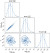 |
Fig. D.1. Constraints on the dark-matter density profile of Eridanus 2 in the computational parametrization, assuming CDM, found using CJAM and MultiNest. Units are omitted for clarity. The parameters are the dark-matter densities ρ2 and ρ3 at 100 pc and 150 pc, respectively, in M⊙ kpc−3 and the systemic velocity (v0) in km s−1. The contours correspond to 0.5σ, 1.0σ, 1.5σ, and 2.0σ confidence levels, where σ is the standard deviation of a two-dimensional normal distribution. The vertical dashed lines in the one-dimensional histograms indicate the median and the 68% confidence interval. |
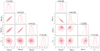 |
Fig. D.2. Constraints on the dark-matter density profile of Eridanus 2 in the computational (left) and astrophysical (right) parametrizations, assuming SIDM, found using CJAM and MultiNest. Units are omitted for clarity. The parameters are the dark-matter densities ρ1, ρ2, and ρ3 at 50 pc, 100 pc, and 150 pc, respectively, in M⊙ kpc−3, the characteristic dark-matter density (ρ0) in M⊙ kpc−3, the scale radius (rs) and core radius (rc) in kpc, and the systemic velocity (v0) in km s−1. The contours correspond to 0.5σ, 1.0σ, 1.5σ, and 2.0σ confidence levels, where σ is the standard deviation of a two-dimensional normal distribution. The vertical dashed lines in the one-dimensional histograms indicate the median and the 68% confidence interval (without arrows) or the 68% and 95% confidence limits (upper and lower arrows, respectively). |
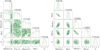 |
Fig. D.3. Constraints on the dark-matter density profile of Eridanus 2 in the computational (left) and astrophysical (right) parametrizations, assuming FDM, found using CJAM and MultiNest. Units are omitted for clarity. The parameters are the dark-matter density of the CDM-like outer profile at 100 pc (ρCDM, 100), the logarithmic slope of the CDM-like outer profile at 100 pc (αCDM, 100), the soliton radius (rsol) in kpc, the scale radius (rs) of the CDM-like outer profile in kpc, the ratio of the dark-matter density at the transition between inner and outer profiles over the central soliton density (ε), the characteristic dark-matter density of the CDM-like outer profile (ρCDM, 0) in M⊙, kpc−3, the central dark-matter density of the soliton (ρsol, 0) in M⊙ kpc−3, and the systemic velocity (v0) in km s−1. The contours correspond to 0.5σ, 1.0σ, 1.5σ, and 2.0σ confidence levels, where σ is the standard deviation of a two-dimensional normal distribution. The vertical dashed lines in the one-dimensional histograms indicate the median and the 68% confidence interval (without arrows) or the 68% and 95% confidence limits (upper and lower arrows, respectively). |
Appendix E: Recovery of intrinsic velocity dispersion profiles
Profiles of the intrinsic velocity dispersion allow a direct comparison between models and data-derived estimates. In Fig. E.1 we display this comparison.
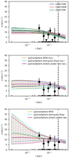 |
Fig. E.1. Recovered intrinsic velocity dispersion profiles of Eridanus 2. Top: CJAM models for CDM, SIDM, and FDM. Centre: pyGravSphere models assuming an isotropic velocity distribution, with NFW, Hernquist–Zhao, and broken power-law profiles. Bottom: as above, without assuming isotropy. Binned intrinsic velocity dispersion estimates are indicated with black circles and error bars, or with downward triangles where negative. The hatched bands represent the 68% confidence interval on the density at each radius. The half-light radius is indicated with the vertical dashed line. The black markers at the bottom of the figure show the projected radii of the kinematic tracers. Tracers in bins rejected by pyGravSphere are marked in grey. |
In addition to the CJAM models with isotropic velocities and the pyGravSphere models with anisotropic velocities used in the main body of this paper, we also display pyGravSphere models with isotropic velocities for comparison. The assumption on the velocity distribution has a large effect on the uncertainty in the intrinsic velocity dispersion at small radii, but in all cases the profiles are consistent with one another within their uncertainties. To compare the recovered profiles to the measured data, we show the estimated intrinsic velocity dispersion and its uncertainty in each pyGravSphere bin. For pyGravSphere we do not display bins with negative estimates (which are unphysical). We remind the reader that CJAM does not bin the velocity data; CJAM does not directly fit to the estimates displayed here. For CJAM we indicate the negative estimates as well.
The intrinsic velocity dispersion profiles clarify the origin of some of the differences in the density profiles. The difference in the scale radius, with CJAM preferring smaller values than pyGravSphere, seems to be driven by the outer bins. The unbinned analysis of CJAM recovers an intrinsic dispersion profile that is lower at large radii, while pyGravSphere prefers models that are flatter. The higher density of the broken power-law profile around 100 pc is also visible in the dispersion profile and seems to be the result of overfitting to the estimators.
All Tables
Quantities derived from the CJAM-MultiNest density or mass profiles of Eridanus 2 under the assumptions of different profile models.
Quantities derived from the pyGravSphere-emcee density or mass profiles of Eridanus 2 under the assumptions of different profile models.
All Figures
|
Fig. 1. Composite-colour image mosaic of Eridanus 2 as observed with MUSE-Faint. Sloan Digital Sky Survey filters g, r, and i were used for the colours blue, green, and red, respectively. Images of the five separately reduced fields were combined with Montage, and the colours were composited using the algorithm from Lupton et al. (2004). The 72 member stars with MUSE-Faint measurements are circled in green. Celestial north is up. The angular and physical scales at the distance of Eridanus 2 are indicated in the bottom left corner. |
| In the text | |
|
Fig. 2. Constraints on the dark-matter density profile of Eridanus 2 in the astrophysical parametrization, assuming CDM, found using CJAM and MultiNest. Units are omitted for clarity. The parameters are the characteristic dark-matter density (ρ0) in M⊙ kpc−3, the scale radius (rs) in kpc, and the systemic velocity (v0) in km s−1. The contours correspond to 0.5σ, 1.0σ, 1.5σ, and 2.0σ confidence levels, where σ is the standard deviation of a two-dimensional normal distribution. The vertical dashed lines in the one-dimensional histograms indicate the median and the 68% confidence interval. |
| In the text | |
|
Fig. 3. Constraints on the dark-matter density profile of Eridanus 2 in the microphysical parametrization, assuming SIDM, found using CJAM and MultiNest. Units are omitted for clarity. The parameters are the characteristic dark-matter density (ρ0) in M⊙ kpc−3, the scale radius (rs) in kpc, the effective self-interaction coefficient (fΓ) in cm3 s−1 eV−1 c2, and the systemic velocity (v0) in km s−1. The contours correspond to 0.5σ, 1.0σ, 1.5σ, and 2.0σ confidence levels, where σ is the standard deviation of a two-dimensional normal distribution. The vertical dashed lines in the one-dimensional histograms indicate the median and the 68% confidence interval (without arrows) or the 68% and 95% confidence limits (upper and lower arrows, respectively). |
| In the text | |
|
Fig. 4. Constraints on the dark-matter density profile of Eridanus 2 in the microphysical parametrization, assuming FDM, found using CJAM and MultiNest. Units are omitted for clarity. The parameters are the characteristic dark-matter density of the CDM-like outer profile (ρCDM, 0) in M⊙ kpc−3, the scale radius (rs) of the CDM-like outer profile in kpc, the dark-matter particle mass (ma) in eV c−2, the transition radius (rt) between the inner soliton and outer CDM-like profile in kpc, and the systemic velocity (v0) in km s−1. The contours correspond to 0.5σ, 1.0σ, 1.5σ, and 2.0σ confidence levels, where σ is the standard deviation of a two-dimensional normal distribution. The vertical dashed lines in the one-dimensional histograms indicate the median and the 68% confidence interval (without arrows) or the 68% and 95% confidence limits (upper and lower arrows, respectively). |
| In the text | |
|
Fig. 5. Constraints on the dark-matter density profile of Eridanus 2, assuming an NFW profile, found using pyGravSphere. Units are omitted for clarity. The parameters are the characteristic dark-matter density (ρ0) in M⊙ kpc−3, the scale radius (rs) in kpc, the symmetrized inner and outer velocity anisotropy ( |
| In the text | |
|
Fig. 6. Constraints on the dark-matter density profile of Eridanus 2, assuming a Hernquist–Zhao profile, found using pyGravSphere. Units are omitted for clarity. The parameters are the characteristic dark-matter density (ρ0) in M⊙ kpc−3, the scale radius (rs) in kpc, the inner and outer negative logarithmic slopes (γ and β) and the sharpness (α) of their transition, the symmetrized inner and outer velocity anisotropy ( |
| In the text | |
|
Fig. 7. Constraints on the dark-matter density profile of Eridanus 2, assuming a broken power-law profile, found using pyGravSphere. Units are omitted for clarity. The parameters are the characteristic dark-matter density (ρ0) in M⊙ kpc−3, the negative power-law slopes (γ0, …, γ4), the symmetrized inner and outer velocity anisotropy ( |
| In the text | |
|
Fig. 8. Recovered dark-matter density profile of Eridanus 2, comparing the CJAM model for CDM with the pyGravSphere NFW profile. These models have the same functional form for the density profile but use different assumptions and methods of calculation. The hatched bands represent the 68% confidence interval on the density at each radius. The half-light radius is indicated with the vertical dashed line. The black markers at the bottom of the figure show the projected radii of the kinematic tracers. Tracers in bins rejected by pyGravSphere are marked in grey. |
| In the text | |
|
Fig. 9. Recovered dark-matter density profile of Eridanus 2. Left: CJAM models for CDM, SIDM, and FDM. Right: pyGravSphere models with NFW, Hernquist–Zhao, and broken power-law profiles. The hatched bands represent the 68% confidence interval on the density at each radius. The half-light radius is indicated with the vertical dashed line. The black markers at the bottom of the figure show the projected radii of the kinematic tracers. Tracers in bins rejected by pyGravSphere are marked in grey. |
| In the text | |
|
Fig. 10. Recovered de-projected mass-to-light profiles of Eridanus 2. These profiles show the local ratio of dark-matter density over luminosity density as a function of radius. The light profile is the exponential profile determined by Crnojević et al. (2016). Left: CJAM models for CDM, SIDM, and FDM. Right: pyGravSphere models with NFW, Hernquist–Zhao, and broken power-law dark-matter profiles. The hatched bands represent the 68% confidence interval on the mass-to-light ratio at each radius. The half-light radius is indicated with the vertical dashed line. The black markers at the bottom of the figure show the projected radii of the kinematic tracers. Tracers in bins rejected by pyGravSphere are marked in grey. |
| In the text | |
|
Fig. D.1. Constraints on the dark-matter density profile of Eridanus 2 in the computational parametrization, assuming CDM, found using CJAM and MultiNest. Units are omitted for clarity. The parameters are the dark-matter densities ρ2 and ρ3 at 100 pc and 150 pc, respectively, in M⊙ kpc−3 and the systemic velocity (v0) in km s−1. The contours correspond to 0.5σ, 1.0σ, 1.5σ, and 2.0σ confidence levels, where σ is the standard deviation of a two-dimensional normal distribution. The vertical dashed lines in the one-dimensional histograms indicate the median and the 68% confidence interval. |
| In the text | |
|
Fig. D.2. Constraints on the dark-matter density profile of Eridanus 2 in the computational (left) and astrophysical (right) parametrizations, assuming SIDM, found using CJAM and MultiNest. Units are omitted for clarity. The parameters are the dark-matter densities ρ1, ρ2, and ρ3 at 50 pc, 100 pc, and 150 pc, respectively, in M⊙ kpc−3, the characteristic dark-matter density (ρ0) in M⊙ kpc−3, the scale radius (rs) and core radius (rc) in kpc, and the systemic velocity (v0) in km s−1. The contours correspond to 0.5σ, 1.0σ, 1.5σ, and 2.0σ confidence levels, where σ is the standard deviation of a two-dimensional normal distribution. The vertical dashed lines in the one-dimensional histograms indicate the median and the 68% confidence interval (without arrows) or the 68% and 95% confidence limits (upper and lower arrows, respectively). |
| In the text | |
|
Fig. D.3. Constraints on the dark-matter density profile of Eridanus 2 in the computational (left) and astrophysical (right) parametrizations, assuming FDM, found using CJAM and MultiNest. Units are omitted for clarity. The parameters are the dark-matter density of the CDM-like outer profile at 100 pc (ρCDM, 100), the logarithmic slope of the CDM-like outer profile at 100 pc (αCDM, 100), the soliton radius (rsol) in kpc, the scale radius (rs) of the CDM-like outer profile in kpc, the ratio of the dark-matter density at the transition between inner and outer profiles over the central soliton density (ε), the characteristic dark-matter density of the CDM-like outer profile (ρCDM, 0) in M⊙, kpc−3, the central dark-matter density of the soliton (ρsol, 0) in M⊙ kpc−3, and the systemic velocity (v0) in km s−1. The contours correspond to 0.5σ, 1.0σ, 1.5σ, and 2.0σ confidence levels, where σ is the standard deviation of a two-dimensional normal distribution. The vertical dashed lines in the one-dimensional histograms indicate the median and the 68% confidence interval (without arrows) or the 68% and 95% confidence limits (upper and lower arrows, respectively). |
| In the text | |
|
Fig. E.1. Recovered intrinsic velocity dispersion profiles of Eridanus 2. Top: CJAM models for CDM, SIDM, and FDM. Centre: pyGravSphere models assuming an isotropic velocity distribution, with NFW, Hernquist–Zhao, and broken power-law profiles. Bottom: as above, without assuming isotropy. Binned intrinsic velocity dispersion estimates are indicated with black circles and error bars, or with downward triangles where negative. The hatched bands represent the 68% confidence interval on the density at each radius. The half-light radius is indicated with the vertical dashed line. The black markers at the bottom of the figure show the projected radii of the kinematic tracers. Tracers in bins rejected by pyGravSphere are marked in grey. |
| In the text | |
Current usage metrics show cumulative count of Article Views (full-text article views including HTML views, PDF and ePub downloads, according to the available data) and Abstracts Views on Vision4Press platform.
Data correspond to usage on the plateform after 2015. The current usage metrics is available 48-96 hours after online publication and is updated daily on week days.
Initial download of the metrics may take a while.