| Issue |
A&A
Volume 651, July 2021
|
|
|---|---|---|
| Article Number | A60 | |
| Number of page(s) | 10 | |
| Section | The Sun and the Heliosphere | |
| DOI | https://doi.org/10.1051/0004-6361/201935774 | |
| Published online | 13 July 2021 | |
Observation of bi-directional jets in a prominence⋆
1
CEMPS, University of Exeter, Exeter EX4 4QF, UK
e-mail: This email address is being protected from spambots. You need JavaScript enabled to view it.
2
Bay Area Environmental Research Institute, NASA Research Park, Moffett Field, CA 94035, USA
3
Lockheed Martin Solar & Astrophysics Laboratory, Org. A021S, Bldg. 252, 3251 Hanover St., Palo Alto, CA 94304, USA
Received:
25
April
2019
Accepted:
29
April
2021
Abstract
Quiescent prominences host a large range of flows, many driven by buoyancy, which lead to velocity shear. The presence of these shear flows could bend and stretch the magnetic field resulting in the formation of current sheets which can lead to magnetic reconnection. Though this has been hypothesised to occur in prominences, with some observations that are suggestive of this process, clear evidence has been lacking. In this paper we present observations performed on June 30, 2015 using the Interface Region Imaging Spectrograph Si IV and Mg II slit-jaw imagers of two bi-directional jets that occur inside the body of the prominence. Such jets are highly consistent with what would be expected from magnetic reconnection theory. Using this observation, we estimate that the prominence under study has an ambient field strength in the range of 4.5−9.2 G with ‘turbulent’ field strengths of 1 G. Our results highlight the ability of gravity-driven flows to stretch and fold the magnetic field of the prominence, implying that locally, the quiescent prominence field can be far from a static, force-free magnetic field.
Key words: magnetic reconnection / magnetohydrodynamics (MHD) / Sun: filaments, prominences / Sun: magnetic fields
Movies are available at https://www.aanda.org
© ESO 2021
1. Introduction
Quiescent prominences are cool, dense clouds of plasma that form in the hot solar corona. On their largest scale, quiescent prominences can be very stable, existing in the corona for weeks. However, they play host to a large range of flow dynamics over a wide range of spatial and temporal scales including downflows and vortices (e.g. Engvold 1981; Kubota & Uesugi 1986; Liggett & Zirin 1984).
The launch of the Hinode satellite (Kosugi et al. 2007) with the Solar Optical Telescope (SOT; Tsuneta et al. 2008) shed new light on the dynamics of prominence material. Most notable of this is examples of plumes, originally observed by Stellmacher & Wiehr (1973) and rediscovered by Berger et al. (2008) and de Toma et al. (2008), which are thought to be created through the magnetic Rayleigh-Taylor instability (Berger et al. 2008, 2010; Ryutova et al. 2010; Hillier et al. 2012a; Hillier 2018). It is not just upflows that have been observed in prominences, but also supersonic (∼10−20 km s−1) downflows that can be seen to fall downwards in the plane-of-sky (e.g. Berger et al. 2008; Chae 2010). Schmieder et al. (2010) used Doppler measurements of prominence flows combined with plane-of-sky velocities and concluded that the observed downflows are possibly just the projection of flows along the magnetic field, which would imply that at least some of the observed downflows would result from the accretion of cool material into the prominence. The observed dynamic motions have been found to be important for the excitation of turbulence in prominences (Leonardis et al. 2012; Freed et al. 2016; Hillier et al. 2017).
Further developments in the study of prominences have been made with the New Vacuum Solar Telescope (NVST, Liu et al. 2014). The use of NVST observations has allowed a further look at the dynamic motions in prominences, showing new information on upflows (Shen et al. 2015) and the development of vortices (Li et al. 2018) in prominences. Using data from NVST, Bi et al. (2020) present observations of knots, finding that the majority descended downwards across the horizontal magnetic field, and they conjecture that the Alfvén waves these motions would excite could contribute to the heating of the corona near the prominence.
In a quiescent prominence, the characteristic temperatures (∼104 K), densities (∼10−13 g cm−3), and magnetic field strengths (3−10 G) produce a low plasma β environment (Tandberg-Hanssen 1995). This can lead to the misconception that only the Lorentz force can be important for driving the observed dynamic motions. However, to explain how flows develop it is important to understand that the ratio between gravity and magnetic tension (Hillier 2018), which can be of order 1 in quiescent prominences (Hinode Review Team 2019), is the key determining factor in whether the prominence material can become dynamic.
The existence of the observed flows could work to distort the magnetic field of the prominence leading to current sheet formation, and with it magnetic reconnection. There have been a number of examples reported of flows in prominences that are hypothesised to be driven by magnetic reconnection. Chae (2010) presented observations of prominence knots that travelled downward in the prominence at speeds of ∼10 km s−1. They conjectured these were caused by reconnection in a setting similar to that proposed by Petrie & Low (2005), where differences in the curvature of the supporting magnetic field result in current sheet formation, leading to reconnection that breaks the force-balance resulting in downflows. A similar dynamic was found in the simulations of Hillier et al. (2012b), where downflows were caused by reconnection in current sheets, and developed slow-mode MHD shocks that pulled down the magnetic field as the plasma fell. Hillier et al. (2011) used Hinode SOT to analyse upward ejections from the top of a quiescent prominence, finding them to be impulsively ejected at supersonic speeds, with the authors proposing reconnection as the acceleration mechanism for the plasma blobs due to their supersonic ejection speeds. On a larger scale, Mishra et al. (2020) present observations of vortical motions that led to the global separation of a prominence resulting in magnetic reconnection to occur. A clear signature of magnetic reconnection occurring in prominences would be the presence of bi-directional ejections. However, these observations are still lacking.
The Interface Region Imaging Spectrograph (IRIS; De Pontieu et al. 2014) provides spectra and images of the cool chromospheric plasma observed in prominences with high spatial (0.33−0.4″), spectral (down to 1−2 km s−1) and temporal resolution (down to 1−2 s), making it a powerful instrument in the investigation of prominence dynamics (e.g. Schmieder et al. 2014). Okamoto et al. (2016) use IRIS spectra and slit-jaw images to determine the 3D velocity field of motions in a prominence, revealing the helical structure of that prominence’s magnetic field. Though in a separate observation, what appears to be helical motion of prominence material could be understood as motion parallel to the solar surface that appeared helical when projected onto a 2D plane (Schmieder et al. 2017). Hillier & Polito (2018) discovered the formation of the Kelvin-Helmholtz instability driven by the complex flows found in the body of a prominence using IRIS slit-jaw images. These observations complement the dynamic nature of prominences found in simulations of small-scale prominence dynamics inside a large prominence body (Xia & Keppens 2016a,b; Kaneko & Yokoyama 2018).
In this paper we analyse a highly dynamic region of a quiescent prominence observed by IRIS. We find two examples of a bi-directional ejection that we interpret as the observational signature of small-scale reconnection jets in the prominence. In conjunction with this observational evidence of reconnection, we provide theoretical arguments to aid our interpretation.
2. Observations
Since its launch in 2013, IRIS has provided an unprecedented view of the solar chromosphere and transition region thanks to its unique design which includes: a dual-range spectrograph (SG) in the far-ultraviolet (FUV; 1332−1407 Å) and near-ultraviolet (NUV; 2783−2835 Å) observing spectra and continuum at high spatial (0.33−0.4″) and spectral resolution (13 mÅ−26 mÅ); a slit-jaw imager (SJI), providing high resolution (0.167″ pix−1) images in four passbands centred around 1330 Å, 1400 Å, 2796 Å and 2830 Å.
A prominence was observed with IRIS on the south-east limb of the Sun on June 30, 2015 between 6:57 UT and 11:20 UT during three sit and stare studies with gaps of around 10 min in between. These studies include SJI images in the 1400 Å, 1330 Å and 2796 Å filters, with a cadence of ∼96 s, and a sequence of sit and stare spectral rasters with a cadence of ∼30 s. This prominence presents many interesting dynamic features, some of which were previously presented in Hillier & Polito (2018), and we investigate one of particular interest.
Figure 1 shows an image of the prominence at 09:21 UT as observed in the 2796 Å filter, dominated by emission from the chromospheric Mg II k/h lines formed at log(T[K]) ∼ 3.7−4.2, and in the 1400 Å filter, dominated by emission from the transition region Si IV line formed at log(T[K]) ∼ 4.9. The image is in log-intensity scale and the vertical white line overplotted on the image indicates the position of the IRIS spectrograph slit during the observations. Unfortunately, the dynamics presented here are not cospatial with the spectrograph slit and therefore we do not have spectra through which we could determine the line-of-sight velocity component of the dynamic features. Finally, the yellow box in Fig. 1 shows the region displayed in Fig. 2, as described in Sect. 3.1.
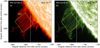 |
Fig. 1. Log intensity image of the prominence seen on 30 June 2015 in the IRIS slitjaw (a) Mg II and (b) Si IV broadband imagers. The yellow box shows the region shown in Fig. 2. The vertical white line shows the position of the IRIS slit. |
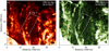 |
Fig. 2. Closeup of the dynamic region at 09:31 UT (we note that the images in the figure have been rotated to set gravity to be in the downward direction). Panel a: Mg II intensity and panel b: Si IV intensity. The white box marks the area used in Fig. 4. The dark line shows the position of the IRIS slit. See online movie of this figure. |
3. Observations of Bi-directional ejections
Figures 2 and 3 show the two events in the prominence we study. The first dynamic event that we focus on occurs in the boxed region shown in Fig. 2, which is an image of the region of interest shown in Fig. 1 taken at 09:31 UT. The dynamic features we analyse are bi-directional ejections from a prominence thread. The observations presented for this event start at 09:13 UT and continue over approximately 30 min. We note that the image in panel b of Fig. 2 has been enhanced with an unsharped mask to show the features more clearly.
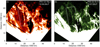 |
Fig. 3. Closeup of the second dynamic region at 10:58 UT (we note that the images in the figure have been rotated to set gravity to be in the downward direction). Panel a: Mg II intensity and panel b: Si IV intensity. The white box marks the area used in Fig. 7. The dark line shows the position of the IRIS slit. See online movie of this figure. |
In the same prominence, a second event presenting similar dynamical features, that is bi-directional ejections was observed. That is to say we see ejections in directions that are roughly anti-parallel as observed in the plane-of-sky from the same position in the prominence. Figure 3 gives the position in the prominence where this event takes place. The observations presented for this event start at 10:15 UT and continue over approximately 65 min.
3.1. Observational analysis of event 1
We first focus on event 1. Figure 4 shows the formation of a plasma sheet which then releases bi-directional ejections along the direction of its axis. The images in each panel of this figure are taken from the white box in Fig. 2. The arrows and lines are used to highlight the important features. A simple description of the temporal evolution is as follows. Firstly, there is a complex interaction between downflows and upflows (a – see movie of Fig. 2). This leads to the development of a thin sheet structure (b). From this sheet structure there are multiple ejections in both directions along the sheet (c, d, e, f, g, h). The sheet intensity dims between ejections marked g and h (j). These dynamics can also be seen in the movie of panel a of Fig. 2. The dashed lines marked (i) and (ii) in the figure are used to show the positions of slits where the intensity is measured in Figs. 5 and 6.
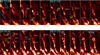 |
Fig. 4. Multiple snapshots in sequence between 09:13:30 and 09:43:47 of the boxed region shown in Fig. 2. The arrows (marked with letters) highlight various dynamics. (a) Direction of the up and down flows in the prominence. (b) The lines delineate the plasma sheet that forms. (c) Ejection from the bottom of the plasma sheet. (d) Ejection from the top of the plasma sheet. (e) Downflow hits flows from plasma sheet and are deflected. (f) Upflow from plasma sheet is deflected and joins the background upflow. (g) Another downward ejection from plasma sheet. (h) Another upward ejection from plasma sheet. (j) a reduction of intensity in the region between the bi-directional ejections (g) and (h). Only the first arrow of any set is marked. The dashed lines marked (i) and (ii) show the positions of the slit used for measuring the plasma sheet width and the time-distance plot in Fig. 6, respectively. See online movie of this figure. |
Figure 5 shows the intensity along the slit (i) as shown in Fig. 4 in both the Mg II and Si IV bands. A Gaussian distribution (dashed line), which we use to estimate the width of the sheet, has been fitted to the intensity, showing that the value of the intensity is approximately 3.5 above the background of 15.5 in the Mg II band and approximately 2.3 above the background of 4.7 for the Si IV band. The Full-Width-Half-Maximum of the distribution is approximately 0.66 arcsec (∼500 km) for both bands. At this time, the length of the sheet is approximately 11.2 arcsec (∼8300 km).
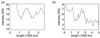 |
Fig. 5. Intensity across the plasma sheet in the (a) Mg II band (averaged over 6 pixels) and (b) Si IV band (averaged over 11 pixels). The position of the slit used to make this diagram is shown as the line marked (i) in Fig. 4. The dashed line is a Gaussian distribution fitted to the intensity. |
The events marked (c), (d), (e), (f), (g) and (h) in Fig. 4 are all ejections that start at the centre of the plasma sheet, moving along the sheet in either direction interacting with the background prominence flows. For four of the blobs the ejections are sufficiently isolated that a 2D Gaussian distribution could be fitted to the Mg II intensity. This allowed for the height and width of the structures to be measured. These results are shown in Table 1. We note that these measurements are taken from one image per blob, and so they provide a characteristic measurement of the blob size but do not describe any temporal evolution.
Parameters of 2D Gaussian fit to blobs.
The motion of some of the blobs appears to be deflected by the background flow. Blobs (e) and (f) show this most clearly. It is hard to remove projection effects from prominences, therefore interaction between different flows provides important evidence that dynamics are co-spatial.
Figure 6 is a time distance diagram made using the vertical slit shown on the bottom panel of Fig. 4 marked (ii). The dashed lines in this figure show the bi-directional outflow along the plasma sheet. They are marked (f), (g) and (h) to match with the blob motions in Fig. 4. The velocities found are 6 km s−1 for (f) and (h) and 10 km s−1 for (g). It is interesting but not surprising that the fastest ejection is in the direction approximately parallel to gravity.
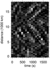 |
Fig. 6. Time-distance diagram using running difference images. The position of the slit used to make this diagram is shown as the line marked (ii) in Fig. 4. The three dashed lines in this figure show the motions of the moving blobs marked (f), (g) and (h) in Fig. 4 with velocities of 6 to 10 km s−1. |
To summarise the observations of this dynamic event, firstly, a long thin plasma sheet develops, and this sheet is ∼8000 km long by ∼600 km wide. Then, in this plasma sheet blobs are ejected in both directions along the length of the sheet. The size of these blobs is ∼1000 km. The speed of these blobs in the plane-of-sky is between 6 and 10 km s−1.
3.2. Observational analysis of event 2
Next we focus on event 2 shown in Fig. 3. In Fig. 7 we show the evolution from the possible formation of a plasma sheet, to multiple plasma blobs ejected both (approximately speaking) in the same direction and in the opposite direction to gravity. The images in each panel of this figure are taken from the white box in Fig. 3. As with the previous example, the arrows and lines are used to highlight the important features. A simple description of the temporal evolution is as follows. Firstly, there is a converging flow (see movie of Fig. 3). This leads to the development of a thin sheet structure (b). From this sheet structure there are multiple ejections in both directions (c, d, e, f, g, h, i j, k, l, m, o, p, q, r, s, t, u). One downflow develops an oscillatory structure (n) – see Sect. 4.2.2 for more details.
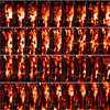 |
Fig. 7. Multiple snapshots of the dynamic ejections. The white arrows marked (a) show the general direction of the approximately up-down motions. The position of the slit used in Fig. 8 is marked (b). What appears to be the initial plasma sheet is highlighted using the two white lines marked (c). A motion of some upwardly ejected blobs – (e), (f), (j), (k), (p), (r), (s) and (v) – and downwardly ejected blobs – (d), (g), (h), (i), (m), (n), (t) and (u) – are marked with white and yellow horizontal arrows respectively. The region inside the blue boxes marked (o) is used in Fig. 9. See online movie of this figure. |
Figure 8 shows the evolution in time of the intensity along the slit marked (b) in Fig. 7. In the brighter material on the right, a number of flows towards the centre are clearly visible. In the darker region on the left, there is at least one flow towards the centre which can be discerned. Using the slopes of these lines we find that these flows have speeds between 2 and 4 km s−1.
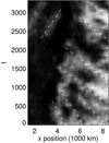 |
Fig. 8. Intensity variation along the slit marked (b) in Fig. 7 with time. The white-black dashed lines are used to highlight the motion of material towards the plasma sheet (marked c in Fig. 7). |
Following the motion of a number of blobs seen in Fig. 7, we find that these blobs move with speeds in the range 10−16 km s−1. These are noticeably larger than the values found for event 1, which could either be as a result of projection effects, or some differences in the physical conditions in the places the blobs are ejected.
4. Theoretical interpretation of the mechanism by which the blobs are formed and ejected
4.1. Highlighting the difference between these dyanmics and previous observed flows
When the Hinode satellite was launched, the seeing-free stable observations revolutionised the study of prominence flows as clear observations could be obtained for significant periods of time. Polar crown prominences in particular were found to be highly dynamic with many upflows and downflows observed. Therefore it is sensible to explicitly clarify why these observations represent a class of flow previously unreported in prominence observations.
The key distinction between observed dynamics presented here and those previously reported is that these flow are bi-directional ejections emitted from the same region (i.e., these are not just upflows and downflows that pass each other at some point). This has not been reported previously, and requires an explanation using a physical process that naturally creates bi-directional ejections. Magnetic reconnection does exactly this. Here we explore the evidence for this mechanism to create the blobs in the next section.
4.2. Interpretation as reconnection jets
In this section we present arguments as to why these observations are created as a result of magnetic reconnection. We look at both events and make connections with reconnection theory to see if we can understand how the observations can be interpreted by magnetic reconnection.
For the first event, these dynamics bear all the hallmarks of the formation of a current sheet (the long, thin structure marked as (b) in Fig. 4) and the subsequent development of magnetic reconnection in that current sheet. The key piece of evidence for this is the existence of bi-directional ejections, a characteristic of magnetic reconnection. In Fig. 4 as the ejections (g) and (h) move away from each other, a low intensity region is formed between them, which could be a sign of the rarefaction that is expected in a reconnection region. Very similar processes can be seen to occur in the second event.
As the magnetic field supporting the prominence material is believed to be initially horizontal then for reconnection to occur, a sufficient angle in the magnetic field would need to be created to allow reconnection to occur. This implies that the flows in the prominence have to have modified the magnetic field, driving the formation of a current sheet that then reconnects. Though others have hypothesised that the dynamics they observed in prominences were created by reconnection, see Sect. 1, we believe these observations present the strongest evidence of this process happening in quiescent prominences so far.
As a first step to lay out the arguments for reconnection to explain the dynamic motions, we can look at how the observed dynamics might connect to magnetic field strengths. One of the most basic components of reconnection theory is that the speed of the reconnection jet is the Alfvén velocity. This would imply that the Alfvén velocity associated with the anti-parallel component of the magnetic field, that is the component that reconnects, is ≈8 km s−1 in the first case or ∼20 km s−1 in the second, as given by the velocity of the ejections. This velocity is trans-sonic, and as this measurement could be smaller than reality as a result of projection effects, it can only be taken as a lower limit for the velocity. Taking this speed as the Alfvén speed of the reconnected field, and a characteristic prominence density of 10−13 g cm−3, we can estimate the strength of the reconnected component of the magnetic field to be  G. It is important to note that this can only be taken as a lower bound for the strength of the reconnected component of the magnetic field because the velocities used to calculate it were only those of the plane-of-sky flows.
In the second event, we have a measure of the speed of both the fast jets being ejected as well as that of the material flowing into the region. In magnetic reconnection, the ratio of the inflow to the outflow gives a measure of the reconnection rate M. For our observations we find this to be ∼0.13 to 0.2. Though this is large, it is similar to the rate found in simulations of two-fluid reconnection in a partially ionised plasma (Leake et al. 2012).
4.2.1. Current-sheet formation
The first example presents what we interpret to be a current sheet has an aspect ratio (width over length) of approximately 0.07. If we assume that the current sheet is supported by magnetic diffusion and that the reconnection is laminar then the Sweet-Parker reconnection scaling law would lead to an estimate of the Lundquist number of 200. Ultimately, this still seems highly unlikely as the expected Lundquist number (S) is approximately, based on the expected Ohmic diffusivity estimated for prominences, 6 orders of magnitude greater than our estimate of 200. Obviously, the estimate of the Lundquist number given by the Sweet-Parker scaling can only be seen as a lower limit due to projection effects, and requires the current sheet to have reached a steady-state reconnection regime that is stable to resistive instabilities. However, to match the Lundquist number estimated from the observations with the value we would theoretically expect if the Sweet-Parker scaling was holding, this would require the sheet structure to be only at an angle to the line-of-sight of ∼1.2° meaning that it has a length of 415 000 km. From these arguments, combined with the width of the sheet being clearly resolved, it is much more likely that for the initial formation of this sheet it is a combination of gas and magnetic pressure that supports it. We can use this assumption to make an attempt to estimate the background conditions in the prominence.
Making the simplifying assumption of a purely horizontal field, and if a shearflow creates a vertical, anti-parallel component of the magnetic field, and using the value of 1 G for this field as estimated earlier using the outflow velocity from event 1, it is possible to make a simple estimate of the ambient field strength of this prominence. If we take the intensity increase in the plasma sheet structure to be only as a result of a density increase (and setting the intensity to scale as ρ2) then through conservation of mass the compression ratio CR can be determined with:
 (1)
(1)
The value of CR is determined to be between 1.1 (Mg II band) to 1.2 (Si IV band). Even though we are using two different spectral lines from two different temperature bands and with very different optical depths, the result is similar. This can be taken as an indication that, as assumed in our estimate, the temperature change is not of critical importance for determining the intensity increase in this case. Obviously, a reason for any discrepancy in the intensity fluctuations is likely to be a result of the difference between optically thick Mg II line and the optically thin Si IV emission (we note that though this line can be considered optically thin in prominences, it is not always optically thin in the solar atmosphere, Kerr et al. 2019).
By considering conservation of magnetic flux, this means the field strength should increase by a factor of 1.1 to 1.2 as well. Taking that the plasma β is likely to be less than 1 (see arguments in introduction) even in this highly dynamic prominence we can approximate the force balance required to stop the current sheet collapse developing further to be purely from magnetic pressure. This results in the following equality for the force balance between the magnetic field outside and inside the current sheet:
 (2)
(2)
where the addition of 1 G on the left-hand side is to show the increased magnetic field outside the current sheet as a result of shearing motions (as discussed in the previous paragraph). Solving this quadratic leads to an estimate of the ambient prominence magnetic field strength of between ∼4.5 G (from Si IV intensity) to ∼9.2 G (from Mg II intensity). We note that the smaller of these two values is associated with a magnetic energy increase that is equivalent of the kinetic energy of a flow at 25 km s−1 assuming a density of 10−13 g cm−3. Therefore, this is a solution that is physically possible in a dynamic quiescent prominence as the velocity difference between up and down-flows can easily exceed 20 km s−1.
We note that this estimated compression should also be associated with a temperature increase, though the difference measured in CR for the two lines may suggest this is small. For adiabatic compression, assuming an adiabatic index of γ = 5/3, we would expect this increase to be by a factor of up to 1.4. As the formation process of the sheet is taking minutes, it is possible that the temperature increase via compression is in part being balanced by radiative losses. Our assumption that the change in intensity is only related to the density may be leading to an over estimation of the compression ratio, which in turn leads to a systematic underestimation of the prominence magnetic field. But it is worth noting that as the value we estimate is highly consistent with many inferred field strengths from spectro-polametric observations (e.g. Leroy 1989; López Ariste et al. 2006; Casini et al. 2009; Schmieder et al. 2013; Orozco Suárez et al. 2014; Levens et al. 2016), it shows that the plasma sheet we observed could easily be a current sheet that forms with support by an internal magnetic field.
4.2.2. Blob formation by reconnection
Now we turn our attention to the blobs that are ejected along the current sheet. There are three possible explanations for the formation of blobs: (1) they are the signature of magnetic islands formed in the current sheet and then ejected, (2) they are slow mode MHD shocks created by a time-dependent reconnection process or (3) they are created by fluid instabilities.
Reconnecting current sheets are susceptible to the formation of magnetic islands (e.g. Huang & Bhattacharjee 2010; Leake et al. 2012; Pucci & Velli 2014). It has been shown that once a reconnecting current sheet develops an aspect ratio of approximately 1/200 (Huang & Bhattacharjee 2010) it becomes unstable to the formation of plasmoids. This ratio was also found to hold for two-fluid simulations of a partially ionised plasma (Leake et al. 2012), which is important to consider as the prominence consists of predominantly neutral material. In dynamically evolving reconnection, the current sheet will thin, and plasmoids will begin to form once the aspect ratio is large enough (Pucci & Velli 2014), estimated for systems with large S to be a ratio that scales as S−1/3, meaning the current sheet does not have to shrink to the Sweet-Parker aspect ratio, given by S−1/2, for plasmoids to form. As shown in Sect. 4.2.1, initially the current sheet has a much larger ratio than the expected Sweet-Parker ratio, and even for the theory of Pucci & Velli (2014) an aspect ratio of 0.07 is consistent with a Lundquist number of ∼3000, which is again much smaller than predicted for the prominence. However, during the reconnection process the current sheet is likely to thin further making plasmoid formation possible. It should be noted that the arguments of Pucci & Velli (2014) can be physically understood as requiring that there is sufficient time for a plasmoid to grow due to the linear instability before it is ejected from the current sheet. If this happens, it could lead to the development of fractal reconnection in the partially ionised prominence plasma (Singh et al. 2015).
The most unstable of the tearing modes grows with a timescale of  where τdiffusion and τAlfven are the diffusion and Alfvén times respectively (both of which are calculated from the thickness of the current sheet). This gives an estimate of τtearing = 108 s for the initial thickness of the plasma sheet. This is significantly longer than the advection time of 104 km/10 km s−1 ≈ 103 s therefore it is unlikely that the instability can grow (Furth et al. 1963; Steinolfson & van Hoven 1984; Tajima & Shibata 2002). This instability would be associated with forming plasmoids of size (e.g. Tajima & Shibata 2002):
 (3)
(3)
where W is the width of the current sheet and taking a Lundquist number of S = 108. From Table 1 the blob size is roughly equivalent to ∼1.5 to 2 × 10³ km. Therefore the predicted plasmoid size is both significantly greater than the observed blob size, and even greater than the length of the initial plasma sheet observed in event 1. To create plasmoids around this size, this would imply the current sheet would have to thin by at least a factor of 20. If the sheet was able to thin this much then the aspect ratio would become small enough to match the cut-off plasmoid formation (e.g. Huang & Bhattacharjee 2010; Leake et al. 2012). Ultimately, these results suggest that the tearing instability is not possible in the initial plasma sheet observed in event 1, but the evolution of reconnection means that this cannot be discounted as a mechanism to create the blobs.
In the arguments we have presented above, we have been purely considering the case where no magnetic field traverses the current sheet, however, in a prominence if the field is sheared by flows it is likely to be the case that such a component of the magnetic field exists. Nishikawa & Sakai (1982) showed that the growth rate for the resistive tearing instability is reduced where there is a component of the magnetic field across the current sheet, with the growth rate becoming comparable to the diffusion time if this component of the field reaches 10% of the ambient field strength. This would imply that such field configurations would not be favourable for explaining the reconnection observed, though they found that non-linear driving of the instability may be able to overcome this problem (Sakai & Nishikawa 1983). One way to reduce the stabilising effect of a transverse field comes from the neutrals that make up the bulk of the prominence material (Hillier et al. 2010).
Another possible explanation of these blobs is that they are the signatures of shocks in the current sheet. In a shock the compression of the fluid would result in an increase in both density and temperature (and with this ionisation state), which would change the intensity possibly explaining why a blob has a higher intensity. Hillier et al. (2012b) showed how reconnection in dynamically forming current sheets in a prominence model resulted in downwardly propagating slow-mode MHD shocks, visible as high-density regions of characteristic width ∼1000 km, very consistent with the observed blob size.
Reconnection shocks can be associated with plasmoids (though not necessarily created by the tearing mode) created as the reconnection jet pushes through a slower moving medium (Zenitani 2015). If reconnection is time dependent as a result of a variable inflow (as would be suggested by the range of flows moving towards the plasma sheet shown in Fig. 8) then this could result in blob formation through shocks created as these regions push through the ambient medium and increase the density and temperature, and with that likely the emission, of the shocked region. The particular nature of the transition inside the shock would be highly influenced by the neutral component of the prominence fluid as shown by the studies by Hillier et al. (2016) and Snow & Hillier (2019).
The other potential explanation for the formation of the blobs as a result of ejection by reconnection is the jet becoming unstable to the Kelvin-Helmholtz instability. Figure 9 shows the zoomed images of the Mg II intensity taken from the blue boxes in Fig. 7. Here we can see a section of the downward propagating jet in event 2. This jet, originally straight, becomes kinked as the jet moves through the background material. As shown in Hillier & Polito (2018) this is the expected when the Kelvin-Helmholtz instability develops on a jet-like flow in a prominence.
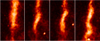 |
Fig. 9. Zoom of the region shown in the blue box in Fig. 7. As this blob moves downward it is found that it develops an undular structure. |
A key aspect of the development of the Kelvin-Helmholtz instability in prominence flows was found to be the aspect ratio by Hillier & Polito (2018). Using the data from the third panel of Fig. 9 we can see that the width (measured from the full-width at half maximum of the intensity) of the flow is ∼0.75 × 10³ km and wavelength of the undulation is ∼2.7 × 10³ km. This is an aspect ratio of ∼3.6, which is very close to the theoretically expected aspect ratio of 3.5 for the Bickley jet (Drazin & Reid 1981), which is a flow of similar profile to the one under study, and consistent with the values found observationally by Hillier & Polito (2018). This gives confirmation to our hypothesis that this undulation is created by the Kelvin-Helmholtz instability.
One aspect of this observed feature that is not consistent with the general image of the Kelvin-Helmholtz is the lack of the undulations growing to become overturning vortices. This can be understood from the work of Hillier (2019) where their Fig. 2 shows a simulation of a KHi unstable MHD flow, but in this situation it is the magnetic field not the fluid flow that results in the non-linear saturation. In this case overturning vortices are not formed by the instability, and it would only be propagating undulations, similar to what can be seen in Fig. 9, which can be observed.
In this section we have looked at three possible explanations for the blob formation: tearing-mode instabilities, shocks and the Kelvin-Helmholtz instability. We are able to rule out the latter as the creator of the blobs as the timescale for the instability to develop is clearly longer than the blob formation timescale. However, evidence that the flowing blobs can become Kelvin-Helmholtz unstable was found in the same observation. For the other two mechanisms, both are possible, and may be working in tandem with each other (e.g. Shibayama et al. 2015; Zhao et al. 2019).
5. Summary and discussion
In this paper we have analysed a prominence observed using the IRIS slitjaw imager in the Mg II and Si IV broadband filters on 30 June 2015. Using these observations we investigated the development of a plasma sheet in which bright blobs formed and were then ejected in both directions along that sheet. We interpreted this event as magnetic reconnection, where the plasma sheet is a current sheet and the blobs ejected are signatures of the reconnection jet. This event is particularly exciting as the represent the first example of these dynamics discovered in prominences.
Using these observed dynamics, and their interpretation, it was possible to give estimates of the field strength of both the prominence and the fluctuating component of the magnetic field. From the observed ejection velocity and a characteristic prominence density, we estimate the reconnected component of the magnetic field to be ∼1 G. Then applying conservation of mass and magnetic flux in conjunction with the formulation of a force balance inside and outside of the plasma sheet, then the ambient prominence magnetic field is estimated to fall in the range of 4.5 G−9.2 G. This magnitude of mean prominence magnetic field combined with a relatively significant turbulent component is consistent with spectro-polarimetric measurements of the magnetic field in a different prominence by Schmieder et al. (2014).
The observations presented in Hillier & Polito (2018) show a shearflow instability developing in the same region of this prominence about one-hour later. For this instability to develop, the magnetic field strength in the plane-of-sky has to give an Alfvén speed that is at least as small as 10 km s−1, but likely to be smaller. This puts an approximate upper limit on the turbulent field for that case of ∼1 G, which highlights that the values estimated in this paper connect to those estimated through other methods for the same prominence. By applying the reconnection models of plasmoid formation and slow-mode MHD shocks, we found that both could explain aspects of the observed ejected blobs but there was insufficient information to determine a prime candidate.
Due to the complexity of the observed dynamics, one simple conclusion that can be made from these observations is that the flows cannot be just simple flows aligned with the magnetic field, but there are flows in prominences with strong components perpendicular to the field that are able to stretch and fold the magnetic field to some extent. As such it is necessary to acknowledge that to stretch the magnetic field in the observed way, these flows have to possess non-negligible kinetic energy when compared to the magnetic energy. From this we can say that not only magnetic forces, but also the forces driving the flows, for example buoyancy forces, are both important in quiescent prominence dynamics and for determining the local structure of the magnetic field.
As with the discovery of prominence plumes (e.g. Berger et al. 2008), it is likely that now these features have been presented many other examples will soon be discovered. We will look for more observations of these phenomena with the aim of capturing them with the spectrograph, so we are able to understand the 3D velocity field, provide a more detailed analysis of the current sheet structure, and potentially investigate heating driven by these dynamics.
Movies
Movie 1 associated with Fig. 2 (Movie_fig2) Access Supplementary Material
Movie 2 associated with Fig. 3 (Movie_fig3) Access Supplementary Material
Movie 3 associated with Fig. 4 (Movie_fig4) Access Supplementary Material
Movie 4 associated with Fig. 7 (Movie_fig7) Access Supplementary Material
Acknowledgments
IRIS is a NASA small explorer mission developed and operated by LMSAL with mission operations executed at NASA Ames Research center and major contributions to downlink communications funded by ESA and the Norwegian Space Centre. The authors would like to thank Dr. Helen Mason and Dr. Giulio Del Zanna for insightful discussions. This work began when both the authors were based at DAMTP, University of Cambridge. the authors thank Dr. S. Jaeggli for planning and performing the observations, and bringing this wonderful data set to our attention. AH acknowledges support by STFC grant ST/R000891/1 and his STFC Ernest Rutherford Fellowship grant number ST/L00397X/2. V.P. acknowledges support by NASA contract NNG09FA40C (IRIS).
References
- Berger, T. E., Shine, R. A., Slater, G. L., et al. 2008, ApJ, 676, L89 [Google Scholar]
- Berger, T. E., Slater, G., Hurlburt, N., et al. 2010, ApJ, 716, 1288 [Google Scholar]
- Bi, Y., Yang, B., Li, T., et al. 2020, ApJ, 891, L40 [CrossRef] [Google Scholar]
- Casini, R., López Ariste, A., Paletou, F., & Léger, L. 2009, ApJ, 703, 114 [Google Scholar]
- Chae, J. 2010, ApJ, 714, 618 [NASA ADS] [CrossRef] [Google Scholar]
- De Pontieu, B., Title, A. M., Lemen, J. R., et al. 2014, Sol. Phys., 289, 2733 [NASA ADS] [CrossRef] [Google Scholar]
- de Toma, G., Casini, R., Burkepile, J. T., & Low, B. C. 2008, ApJ, 687, L123 [CrossRef] [Google Scholar]
- Drazin, P. G., & Reid, W. H. 1981, Hydrodynamic Stability, 2nd ed. (Cambridge: Cambridge University Press) [Google Scholar]
- Engvold, O. 1981, Sol. Phys., 70, 315 [NASA ADS] [CrossRef] [Google Scholar]
- Freed, M. S., McKenzie, D. E., Longcope, D. W., & Wilburn, M. 2016, ApJ, 818, 57 [Google Scholar]
- Furth, H. P., Killeen, J., & Rosenbluth, M. N. 1963, Phys. Fluids, 6, 459 [Google Scholar]
- Hillier, A. 2018, Rev. Mod. Plasma Phys., 2, 1 [Google Scholar]
- Hillier, A. 2019, Phys. Plasmas, 26, 082902 [Google Scholar]
- Hillier, A., & Polito, V. 2018, ApJ, 864, L10 [Google Scholar]
- Hillier, A., Shibata, K., & Isobe, H. 2010, PASJ, 62, 1231 [CrossRef] [Google Scholar]
- Hillier, A., Isobe, H., & Watanabe, H. 2011, PASJ, 63, 19 [CrossRef] [Google Scholar]
- Hillier, A., Berger, T., Isobe, H., & Shibata, K. 2012a, ApJ, 746, 120 [NASA ADS] [CrossRef] [Google Scholar]
- Hillier, A., Isobe, H., Shibata, K., & Berger, T. 2012b, ApJ, 756, 110 [NASA ADS] [CrossRef] [Google Scholar]
- Hillier, A., Takasao, S., & Nakamura, N. 2016, A&A, 591, A112 [NASA ADS] [CrossRef] [EDP Sciences] [Google Scholar]
- Hillier, A., Matsumoto, T., & Ichimoto, K. 2017, A&A, 597, A111 [NASA ADS] [CrossRef] [EDP Sciences] [Google Scholar]
- Hinode Review Team (Al-Janabi, K., et al.) 2019, PASJ, 71, R1 [CrossRef] [Google Scholar]
- Huang, Y.-M., & Bhattacharjee, A. 2010, Phys. Plasmas, 17, 062104 [Google Scholar]
- Kaneko, T., & Yokoyama, T. 2018, ApJ, 869, 136 [Google Scholar]
- Kerr, G. S., Carlsson, M., Allred, J. C., Young, P. R., & Daw, A. N. 2019, ApJ, 871, 23 [CrossRef] [Google Scholar]
- Kubota, J., & Uesugi, A. 1986, PASJ, 38, 903 [NASA ADS] [Google Scholar]
- Kosugi, T., Matsuzaki, K., Sakao, T., et al. 2007, Sol. Phys., 243, 3 [Google Scholar]
- Leake, J. E., Lukin, V. S., Linton, M. G., et al. 2012, ApJ, 760, 109 [NASA ADS] [CrossRef] [Google Scholar]
- Leonardis, E., Chapman, S. C., & Foullon, C. 2012, ApJ, 745, 185 [Google Scholar]
- Leroy, J. L. 1989, Dynamics and Structure of Quiescent Solar Prominences (Dordrecht: Kluwer), 150, 77 [NASA ADS] [CrossRef] [Google Scholar]
- Levens, P. J., Schmieder, B., López Ariste, A., et al. 2016, ApJ, 826, 164 [Google Scholar]
- Li, D., Shen, Y., Ning, Z., et al. 2018, ApJ, 863, 192 [NASA ADS] [CrossRef] [Google Scholar]
- Liggett, M., & Zirin, H. 1984, Sol. Phys., 91, 259 [NASA ADS] [CrossRef] [Google Scholar]
- Liu, Z., Xu, J., Gu, B.-Z., et al. 2014, Res. Astron. Astrophys., 14, 705 [Google Scholar]
- López Ariste, A., Aulanier, G., Schmieder, B., & Sainz Dalda, A. 2006, A&A, 456, 725 [NASA ADS] [CrossRef] [EDP Sciences] [Google Scholar]
- Mishra, S. K., Srivastava, A. K., & Chen, P. F. 2020, Sol. Phys., 295, 167 [CrossRef] [Google Scholar]
- Nishikawa, K.-I., & Sakai, J. 1982, Phys. Fluids, 25, 1384 [CrossRef] [Google Scholar]
- Okamoto, T. J., Liu, W., & Tsuneta, S. 2016, ApJ, 831, 126 [NASA ADS] [CrossRef] [Google Scholar]
- Orozco Suárez, D., Díaz, A. J., Asensio Ramos, A., & Trujillo Bueno, J. 2014, ApJ, 785, L10 [Google Scholar]
- Petrie, G. J. D., & Low, B. C. 2005, ApJS, 159, 288 [NASA ADS] [CrossRef] [Google Scholar]
- Pucci, F., & Velli, M. 2014, ApJ, 780, L19 [CrossRef] [Google Scholar]
- Ryutova, M., Berger, T., Frank, Z., Tarbell, T., & Title, A. 2010, Sol. Phys., 267, 75 [Google Scholar]
- Sakai, J., & Nishikawa, K.-I. 1983, Sol. Phys., 88, 241 [CrossRef] [Google Scholar]
- Schmieder, B., Chandra, R., Berlicki, A., & Mein, P. 2010, A&A, 514, A68 [NASA ADS] [CrossRef] [EDP Sciences] [Google Scholar]
- Schmieder, B., Kucera, T. A., Knizhnik, K., et al. 2013, ApJ, 777, 108 [Google Scholar]
- Schmieder, B., Tian, H., Kucera, T., et al. 2014, A&A, 569, A85 [NASA ADS] [CrossRef] [EDP Sciences] [Google Scholar]
- Schmieder, B., Zapiór, M., López Ariste, A., et al. 2017, A&A, 606, A30 [NASA ADS] [CrossRef] [EDP Sciences] [Google Scholar]
- Shen, Y., Liu, Y., Liu, Y. D., et al. 2015, ApJ, 814, L17 [NASA ADS] [CrossRef] [Google Scholar]
- Shibayama, T., Kusano, K., Miyoshi, T., et al. 2015, Phys. Plasmas, 22, 100706 [NASA ADS] [CrossRef] [Google Scholar]
- Singh, K. A. P., Hillier, A., Isobe, H., & Shibata, K. 2015, PASJ, 67, 96 [NASA ADS] [CrossRef] [Google Scholar]
- Snow, B., & Hillier, A. 2019, A&A, 626, A46 [NASA ADS] [CrossRef] [EDP Sciences] [Google Scholar]
- Stellmacher, G., & Wiehr, E. 1973, A&A, 24, 321 [Google Scholar]
- Steinolfson, R. S., & van Hoven, G. 1984, Phys. Fluids, 27, 1207 [CrossRef] [Google Scholar]
- Tajima, T., & Shibata, K. 2002, Plasma Astrophysics (Cambridge, MA: Perseus) [Google Scholar]
- Tandberg-Hanssen, E. 1995, Astrophys. Space Sci. Lib. (Dordrecht: Kluwer Academic Publishers), 199 [Google Scholar]
- Tsuneta, S., Ichimoto, K., Katsukawa, Y., et al. 2008, Sol. Phys., 249, 167 [NASA ADS] [CrossRef] [Google Scholar]
- Xia, C., & Keppens, R. 2016a, ApJ, 825, L29 [Google Scholar]
- Xia, C., & Keppens, R. 2016b, ApJ, 823, 22 [Google Scholar]
- Zenitani, S. 2015, Phys. Plasmas, 22, 032114 [CrossRef] [Google Scholar]
- Zhao, X., Xia, C., Van Doorsselaere, T., et al. 2019, ApJ, 872, 190 [CrossRef] [Google Scholar]
All Tables
All Figures
|
Fig. 1. Log intensity image of the prominence seen on 30 June 2015 in the IRIS slitjaw (a) Mg II and (b) Si IV broadband imagers. The yellow box shows the region shown in Fig. 2. The vertical white line shows the position of the IRIS slit. |
| In the text | |
|
Fig. 2. Closeup of the dynamic region at 09:31 UT (we note that the images in the figure have been rotated to set gravity to be in the downward direction). Panel a: Mg II intensity and panel b: Si IV intensity. The white box marks the area used in Fig. 4. The dark line shows the position of the IRIS slit. See online movie of this figure. |
| In the text | |
|
Fig. 3. Closeup of the second dynamic region at 10:58 UT (we note that the images in the figure have been rotated to set gravity to be in the downward direction). Panel a: Mg II intensity and panel b: Si IV intensity. The white box marks the area used in Fig. 7. The dark line shows the position of the IRIS slit. See online movie of this figure. |
| In the text | |
|
Fig. 4. Multiple snapshots in sequence between 09:13:30 and 09:43:47 of the boxed region shown in Fig. 2. The arrows (marked with letters) highlight various dynamics. (a) Direction of the up and down flows in the prominence. (b) The lines delineate the plasma sheet that forms. (c) Ejection from the bottom of the plasma sheet. (d) Ejection from the top of the plasma sheet. (e) Downflow hits flows from plasma sheet and are deflected. (f) Upflow from plasma sheet is deflected and joins the background upflow. (g) Another downward ejection from plasma sheet. (h) Another upward ejection from plasma sheet. (j) a reduction of intensity in the region between the bi-directional ejections (g) and (h). Only the first arrow of any set is marked. The dashed lines marked (i) and (ii) show the positions of the slit used for measuring the plasma sheet width and the time-distance plot in Fig. 6, respectively. See online movie of this figure. |
| In the text | |
|
Fig. 5. Intensity across the plasma sheet in the (a) Mg II band (averaged over 6 pixels) and (b) Si IV band (averaged over 11 pixels). The position of the slit used to make this diagram is shown as the line marked (i) in Fig. 4. The dashed line is a Gaussian distribution fitted to the intensity. |
| In the text | |
|
Fig. 6. Time-distance diagram using running difference images. The position of the slit used to make this diagram is shown as the line marked (ii) in Fig. 4. The three dashed lines in this figure show the motions of the moving blobs marked (f), (g) and (h) in Fig. 4 with velocities of 6 to 10 km s−1. |
| In the text | |
|
Fig. 7. Multiple snapshots of the dynamic ejections. The white arrows marked (a) show the general direction of the approximately up-down motions. The position of the slit used in Fig. 8 is marked (b). What appears to be the initial plasma sheet is highlighted using the two white lines marked (c). A motion of some upwardly ejected blobs – (e), (f), (j), (k), (p), (r), (s) and (v) – and downwardly ejected blobs – (d), (g), (h), (i), (m), (n), (t) and (u) – are marked with white and yellow horizontal arrows respectively. The region inside the blue boxes marked (o) is used in Fig. 9. See online movie of this figure. |
| In the text | |
|
Fig. 8. Intensity variation along the slit marked (b) in Fig. 7 with time. The white-black dashed lines are used to highlight the motion of material towards the plasma sheet (marked c in Fig. 7). |
| In the text | |
|
Fig. 9. Zoom of the region shown in the blue box in Fig. 7. As this blob moves downward it is found that it develops an undular structure. |
| In the text | |
Current usage metrics show cumulative count of Article Views (full-text article views including HTML views, PDF and ePub downloads, according to the available data) and Abstracts Views on Vision4Press platform.
Data correspond to usage on the plateform after 2015. The current usage metrics is available 48-96 hours after online publication and is updated daily on week days.
Initial download of the metrics may take a while.