| Issue |
A&A
Volume 651, July 2021
|
|
|---|---|---|
| Article Number | A30 | |
| Number of page(s) | 8 | |
| Section | Interstellar and circumstellar matter | |
| DOI | https://doi.org/10.1051/0004-6361/201935739 | |
| Published online | 06 July 2021 | |
[CII] emission properties of the massive star-forming region RCW 36 in a filamentary molecular cloud
1
Graduate School of Science, Nagoya University,
Furo-cho, Chikusa-ku, Nagoya,
Aichi
464-8602,
Japan
e-mail: This email address is being protected from spambots. You need JavaScript enabled to view it.
2
Tata Institute of Fundamental Research,
Homi Bhabha Road, Colaba,
Mumbai
400005,
India
3
Institute of Space and Astronautical Science, Japan Aerospace Exploration Agency 3-1-1 Yoshinodai, Chuo-ku, Sagamihara,
Kanagawa
252-5210,
Japan
4
The Pennsylvania State University, University Park,
State College,
PA,
USA
5
Indian Institute of Space Science and Technology,
Valiamala,
Thiruvananthapuram
695 547,
India
Received:
19
April
2019
Accepted:
25
February
2021
Abstract
Aims. We investigate the properties of [C II] 158 μm emission of RCW 36 in a dense filamentary cloud.
Methods. [C II] observations of RCW 36, covering an area of ~30′ × 30′, were carried out with a Fabry-Pérot spectrometer on board a 100-cm balloon-borne far-infrared (IR) telescope with an angular resolution of 90′′. Using AKARI and Herschel images, we compared the spatial distribution of the [C II] intensity with the emission from the large grains and polycyclic aromatic hydrocarbon (PAH).
Results. The [C II] emission is in good spatial agreement with shell-like structures of a bipolar lobe observed in IR images, which extend along the direction perpendicular to the direction of cold dense filament. We found that the [C II]–160 μm relation for RCW 36 shows a higher brightness ratio of [C II]/160 μm than that for RCW 38, while the [C II]–9 μm relation for RCW 36 is in good agreement with that for RCW 38.
Conclusions. Via a spectral decomposition analysis on a pixel-by-pixel basis using IR images, the [C II] emission is spatially well correlated with PAH and cold dust emissions. This means that the observed [C II] emission predominantly comes from photo-dissociation regions. Moreover, the L[C II]∕LFIR ratio shows large variation (10−2–10−3), as compared with the L[C II]/LPAH ratio. In view of the observed tight correlation between L[C II]∕LFIR and the optical depth at λ = 160 μm, the large variation in L[C II]∕LFIR can be simply explained by the geometrical effect, that is, LFIR has contributions from the entire dust-cloud column along the line of sight, while L[C II] has contributions from far-UV illuminated cloud surfaces. Based on the picture of the geometry effect, the enhanced brightness ratio of [C II]/160 μm is attributed to the difference in gas structures where massive stars are formed: filamentary (RCW 36) and clumpy (RCW 38) molecular clouds; thus suggesting that RCW 36 is dominated by far-UV illuminated cloud surfaces, as compared with RCW 38.
Key words: dust, extinction / ISM: lines and bands / HII regions / ISM: individual objects: RCW36
© ESO 2021
1 Introduction
The understanding of galaxy evolution is a key subject in modern astrophysics. Massive stars (≳8 M⊙) have a great influence on the evolution of the interstellar medium (ISM) energetically, chemically, and dynamically, thus playing a vital role in galaxy evolution. More recently, Herschel observations revealed the presence of ubiquitous filamentary structures connecting Galactic star-forming regions with each other, suggesting that filaments play a crucial role in star formation (e.g. Molinari et al. 2010; André et al. 2010). Special attention has been placed on filament structures, prompting investigations of the radiative feedback of massive stars on their filamentary ISM (which regulates subsequent star formation) as well as the role of filaments in the formation of dense star-forming clumps (Zinnecker & Yorke 2007; Myers 2009; André et al. 2010; Baug et al. 2015; Dewangan et al. 2017a,b).
A photo-dissociation region (PDR) is formed around an H II region by massive stars, and serves as the region where far-ultraviolet (UV) (6 < hν < 13.6 eV) photons play a significant role in the heating and chemistry of the ISM; all of the atomic and at least 90% of the molecular gas in the Milky Way is contained in PDRs (Hollenbach & Tielens 1999). This means that PDRs are key to understanding the physical properties of the ISM, which is strongly influenced by the radiative feedback of massive stars and the triggering ofnext-generation stars. In PDRs, the gas heating is mainly caused by photoelectrons (photoelectric heating) from dust grains and polycyclic aromatic hydrocarbons (PAHs), which are ejected as they absorb far-UV photons from stars, while the gas cooling is performed by far-infrared (IR) fine-structure lines, among which [C II] 158 μm is the most important gas coolant in low-density PDRs (e.g. Hollenbach & Tielens 1999).
Studies of gas cooling and photo-electric heating of the gas in PDRs require [C II] and IR photometric data sets and sufficient spatial resolution to trace the variety of dust emission components such as PAHs, warm (~ 60–100 K), and cold (~20–30 K) dust emissions. In addition they serve to diagnose region-by-region physical conditions in the ISM. The reason for this is that gas heating and cooling processes depend on dust grain types and ISM conditions. Although Herschel and SOFIA enable us to have an opportunity to access such data sets for the first time, achieving spatial coverage large enough to include an entire Galactic star-formingregion is still lacking for the purposes of a more global understanding of PDRs, particularly in terms of a [C II] map.
RCW 36 is a Galactic massive star-forming region formed in a filament structure of the Vela C molecular cloud complex (Hill et al. 2011); the H II region isformed by ~350 stars, including two O-type and one B-type stars (Ellerbroek et al. 2013). Recent CO observations suggest that massive stars were formedby a cloud-cloud collision along the filament direction (Sano et al. 2018). The composite IR image in Fig. 1 shows two major features in addition to the filament structure: (1) a bipolar lobe with shell-like structures extending the east-west direction, which is perpendicular to the filament structure; (2) a ring-like structure (dashed ellipse) with a major axis of 2 pc at its center. The two features are attributed to a blowout of the filament structure towards surrounding low-density regions because of intense ionising radiation and stellar winds from massive stars (Minier et al. 2013). Thus, RCW 36, with its spectacular features, offers us the best laboratory for exploring the radiative feedback from massive stars. In this paper, the distance to RCW 36 is taken to be 1.09 kpc (Gaia Collaboration 2018).
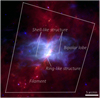 |
Fig. 1 [C II] observation area (solid box) of RCW 36 superimposed on a composite image shown with the equatorial J2000 coordinate system: AKARI 9 μm (blue), Herschel 70 μm (green), and Herschel 250 μm (red). RCW 36 is formed in a large-scale filament extending north-south direction. A bipolar lobe, shell-like structures and a ring-like structure (black dashed ellipse) are identified by Minier et al. (2013). |
2 Observations and data analysis
2.1 [CII] 158 μm data from T100
We carried out [C II] observations of RCW 36 on 15 Nov. 2004, 30 Nov. 2017, and 28 Oct. 2018 by a Fabry-Pérot spectrometer on board a 100-cm balloon-borne far-IR telescope with an angular resolution of 90′′ (hereafter FPS100: Ghosh et al. 1988; Nakagawa et al. 1998). At the Hyderabad Balloon Facility of the Tata Institute of Fundamental Research (TIFR) in India, FPS100 was launched into the stratosphere of an altitude of ~ 30 km. RCW 36 was then observed with a spatially unchopped, fast spectral scan mode by two sets of the spatial raster scans covering a large-scale area of ~30′ × 30′ in total (Fig. 1); detailed descriptions on FPS100 and its observation modes can be found in Mookerjea et al. (2003). Telescope pointing to the science target was achieved by offsetting it with reference to a nearby bright guide star and the absolute pointing error is estimated to be typically ~ 60′′. [C II] flux calibrations were made with Orion B by comparing its [C II] map, taken by Kuiper Airborne Observatory (Jaffe et al. 1994); the flux calibration error is ~10%.
The data reduction follows the same method as in Kaneda et al. (2013); a [C II] intensity map was obtained by subtracting atmospheric background and astronomical continuum emission components from each spectrum scan. For each set of the spatial scans taken in 2004, 2017, and 2018, an atmospheric background spectrum was estimated by averaging the spectral scan data at the eastern edge of the spatial scan legs every three legs; an area of ~ 30′ × 7′ was used as the background region where no significant [C II] line emission from RCW 36 was detected. Then, we fitted the spectral scan data on the corresponding spatial scans by a combination of the atmospheric background spectrum, a Rayleigh-Jeans regime modified black-body function with an emissivity power-law index (β) of 2.0 for an astronomical 158 μm continuum emission, and a Lorentzian function for the [C II] emission. Amplitudes of the atmospheric background, the astronomical 158 μm continuum, and [C II] emission components were set to be free, while the center and the width of the Lorentzian function were fixed to the values estimated from the data of several spectral scans with high signal-to-noise ratio. To determine the positional offset in a [C II] map, we shifted the 158 μm continuum emission map along the RA and Dec axes so that the peak in the continuum emission map is matched to that in a Herschel 160 μm map. Finally, the combined [C II] map obtained from the three maps was regridded with pixel sizes of 90′′ for pixel-by-pixel correlation analyses. This ensures measurements for every pixel to be independent samples (without coupling with the neighbouring pixels).
2.2 Broad-band IR data from AKARI and Herschel
RCW 36 was observed with the AKARI all-sky survey in mid-IR wavelengths (Onaka et al. 2007; Ishihara et al. 2010) and Herschel as part of the Herschel imaging survey of OB young stellar objects (HOBYS) guaranteed time key program (Hill et al. 2011). For the purposes of comparison with the [C II] map, we used two-band images from AKARI (9 and 18 μm) and five-band images from Herschel (70, 160, 250, 350, and 500 μm).
The spatial resolutions of AKARI 9 and 18 μm are 12 and 14′′, respectively. The flux calibration uncertainty of the two bands is ~ 10% (Ishihara et al., in prep.). The Herschel data were taken from the Herschel Science Archive. The Herschel/PACS and SPIRE data are level-2.5 products (SPG version 14.2.0), providing JScanam maps, and level-2 products (SPG version 14.1.0), providing Naive maps, respectively. The beam size has a full width at half maximum (FWHM) of 5, 11, 18, 24, and 35′′ at Herschel 70, 160, 250, 350, and 500 μm, respectively.The systematic flux calibration uncertainty of the Herschel bands is applied to be ~ 5% (PACS Observer’s Manual version 2.5.1 and SPIRE Observer’s Manual version 2.5).
A background level for each of the seven-band IR images was estimated by averaging pixel values in a region where no significant [C II] emission was detected to subtract a diffuse component that is not associated with RCW 36 from each image. The background level is 0.6 (AKARI 9), 0.2 (AKARI 18), 0.1 (Herschel 70), 0.4 (Herschel 160), 3 (Herschel 250), 4 (Herschel 350), and 5% (Herschel 500 μm) of the peak surface brightness. For multi-band analysis, the spatial resolutions of background-subtracted IR images were reduced to match a Gaussian PSF with the FWHM of 90′′ for the FPS100 data by convolving PACS and SPIRE-band images with kernels provided by Aniano et al. (2011). Because such kernels for the AKARI bands are currently not available in the library1, the AKARI images were convolved by a Gaussian kernel to approximate the FPS100 PSF. Then, the convolved images were regridded with a pixel size of 90′′ matched with the PSF of the FPS100 data for pixel-by-pixel correlation analyses.
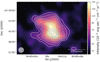 |
Fig. 2 [C II] intensity map of RCW 36 showing an area of 20′ × 15′ taken by FPS100. The contours are linearly spaced 12 levels from 3.3 × 10⁻⁴ to 1.9 × 10⁻³ erg sec−1 cm−2 sr−1. The PSF size in FWHM is shown in the lower-left corner. |
3 Results
3.1 [CII] 158 μm and broadband IR maps
Figure 2 shows the [C II] intensity map of RCW 36 by FPS100. The 1-sigma fluctuation per pixel is 1.1 × 10⁻⁴ erg sec−1 cm−2 sr−1. The [C II] emission overall extends toward the east-west direction from the peak, which is almost perpendicular to the direction of the filament structure as shown in Fig. 1.
The seven-band IR images by AKARI and Herschel are shown in Fig. 3. The AKARI 9 μm image mainly traces emission from PAHs and shows a bipolar lobe with shell-like structures in the east-west direction (Fig. 1). The overall spatial distribution of the AKARI 9 μm map is in good agreement with that of the Herschel 70–500 μm maps that trace emission from large grains, although the Herschel 250–500 μm maps show more prominent filament structure in addition to the bipolar lobe. In the AKARI 18 μm image, which traces emissions from large and very small grains, the spatial distribution also shows the bipolar lobe, but does not show shell-like structures clearly.
To compare spatial distributions between the [C II] map and a broad-band IR emission map, contours of the [C II] intensity are superimposed on each IR map (Fig. 3). The [C II] map shows two prominent arms extending from its peak to the north-east and south-west directions, which are spatially in good agreement with shell-like structures of the bipolar lobe observed in the broadband IR images. The peak position in the [C II] map is located close to the IR bright rims along the ring-like structure (Minier et al. 2013). For a quantitative comparison of spatial distributions, Fig. 4 shows pixel-by-pixel correlation plots of (a) [C II] versus 9 μm and (b) [C II] versus 160 μm. Here, we removed pixels with the optical depth at λ = 9 μm higher than unity from correlation plots. Since the AKARI 9 μm band is overlapping with the interstellar silicate feature around 9.7 μm, the interstellar extinction in the AKARI 9 μm band is the most severe among the seven IR bands. To evaluate the extinction, the optical depth at λ = 9 μm, τ9 is calculated from τ9 = 4.8 × 10⁻²AV by applying A9 ∕AKs = 5.8 × 10⁻¹ (Xue et al. 2016) and AKs∕AV = 8.9 × 10⁻² (Glass 1999); τ9 > 1 corresponds to AV > 21 mag. Hill et al. (2011) investigated an  column density map of the Vela C molecular complex, including RCW 36 on the basis of a pixel-by-pixel SED (spectral energy distribution) fitting in the wavelength range of 70–500 μm. We then converted the
  column density to visual extinction units assuming
 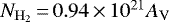 cm−2 (Bohlin et al. 1978). From the map around RCW 36, the regions with AV > 21 mag are located around the peak seen in the Herschel 500 μm map. Therefore, the relevant pixels showing τ9 > 1 were removed. Clearly, the [C II]–9 μm relation for RCW 36 is in good agreement with that for RCW 38 as denoted by black-filled squares, while the [C II]–160 μm relation for RCW 36 shows higher brightness ratio of [C II]/160 μm than that for RCW 38.
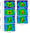 |
Fig. 3 Seven-band images of RCW 36 from the AKARI and Herschel data in (a) AKARI 9 μm, (b) AKARI 18 μm, (c) Herschel 70 μm, (d) Herschel 160 μm, (e) Herschel 250 μm, (f) Herschel 350 μm, and (g) Herschel 500 μm bands. In each image, the colour bar is given in units of MJy sr−1. The PSF size in FWHM is in the lower left corner. The contours superimposed on the images are the same as those in Fig. 2. |
3.2 [CII] 158 μm and molecular gas maps
Sano et al. (2018) presented the latest CO observations of RCW 36 and found two molecular clouds at the velocities VLSR ~ 5.5 km s−1 (blue cloud) and 9 km s−1 (red cloud), which are likely to be physically associated with RCW 36. They also showed that there is no bridge-like feature connecting the two molecular clouds in velocity space. Figure 5 shows 12CO(J = 2−1) contours (Fig. 4a in Sano et al. 2018) overlaid on the [C II] image. The [C II] emission is not spatially in good agreement with the 12CO emission for both red and blue cloud components; the bright 12CO emission from the dense red cloud component has the double peak and its structure is elongated along the filament structure. The double peak is located around the [C II] peak and the massive stars as denoted by the cross marks. Sano et al. (2018) found that the dense red cloud coincides with the star cluster, while the diffuse blue cloud does not. The red cloud seems to be physically close to the star cluster and its proximate surface ionised by the UV radiation from these stars, while the blue cloud is less affected by UV from this cluster due to its far location. Moreover, the diffuse CO emission extending from the filament structure to eastern (red cloud) and western (blue cloud) directions tends to be distributed in the outer rim of shell-like structures seen in [C II] and broadband IR maps.
From the above situation in spatial distributions, we propose a possible geometry of the [C II] emission region with respect to the two collided molecular clouds as follows: for the positional relation among the observer, the red cloud, and the blue cloud, there are two possible cases. The first case is that the red cloud is closer to the observer when the red and blue clouds are colliding with each other, while the second case is that the blue cloud is closer to the observer when the red cloud went through the blue one after collision. As shown in Fukui et al. (2016), the two colliding clouds are generally connected to each other in velocity space and show a bridge-like feature in a position-velocity diagram. Because the bridge-like feature was not observed in RCW36 (Sano et al. 2018), the observational result supports the second case. Therefore, the dense red cloud with the molecular filament went through the blue cloud and is then associated with the massive stars formed by the cloud-cloud collision, while the diffuse red and blue clouds are mostly located the outer rim of shell-like structures. The massive stars formed by the collision between the red and blue clouds illuminate surface of those two clouds. Given that the most of the [C II] emission originates from those far-UV illuminated surface of clouds, the [C II]-emitting region is expected to be facing toward observers without significant attenuation by foreground dust grains associated with CO clouds.
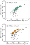 |
Fig. 4 Correlation plots of brightness between (a) [C II] and 9 μm, and (b) [C II]and 160 μm for RCW 36 (circle), together with those for RCW 38 (square) from Fig. 3 in Kaneda et al. (2013). |
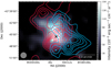 |
Fig. 5 Same as Fig. 2, but 12CO(J = 2–1) contours (Fig. 4a in Sano et al. 2018) and positions of OB stars (cross) (Ellerbroek et al. 2013). The cyan and red coloured contours represent two-velocity molecular cloud components with VLSR = 4.1–6.1 km s−1 (blue cloud) and 7.6–12.0 km s−1 (red cloud), respectively. The spatial resolution of the 12CO(J = 2–1) map taken by NANTEN2 is similar to the [C II] map (90′′). |
4 Discussion
4.1 Spectral decomposition into very cold dust, cold dust, warm dust, and PAH components
Spectral decomposition analysis on a pixel-by-pixel basis enables us to investigate spatial distributions of PAH and dust properties and the relation between those properties and [C II] emission. An individual SED constructed from the seven-band fluxes at each pixel (pixel size of 90′′) is reproduced by a triple-component modified blackbody plus a PAH model expressed as
 (1)
(1)
where T, β, A, and Bν (T) are the dust temperature, the dust emissivity power-law index, amplitude, and the Planck function, respectively. Suffixes vc, c, w, and PAH denote very cold dust, cold dust, warm dust and PAH components, respectively. The β value for each dust component is assumed to be 2.0 as a typical value of the Galactic ISM (Anderson et al. 2012). The second term in the warm dust component is the analytic approximation of thermal emission from dust grains which are exposed to a range of starlight intensities: dust emissions with different dust temperatures assuming a power-law temperature distribution to take the hotdust component into account in mid-IR wavelengths (Casey 2012). The power-law turnover frequency νc defined by Casey (2012) is a function of the mid-IR power-law slope α and Tw. The flux density of the PAH component, FPAH(ν), is calculated as described in Suzuki et al. (2010) and is based on the PAH parameters taken from Li & Draine (2001) and Draine & Li (2007) by assuming the PAH size distribution ranging from 3.55 to 300 Å, the fractional ionisation and the temperature probability distribution for the typical diffuse ISM with the interstellar radiation field in the solar neighbourhood. PAHs with sizes larger than 15 Å contribute to ~ 20 μm continuum emission (Draine & Li 2007). Since very small grains (VSGs), which are stochastically heated by absorbed far-UV photons contribute to ~ 20 μm continuum emission, the PAH component in Eq. (1) takes the VSG emission into account.
The eight free parameters for the SED model cannot be determined from a seven-band data set. We then fixed Tvc and α values obtained from a global SED of RCW 36 by adding IRAS 25, 60, and 100 μm data. Since the parameters Tw and Aw are both determined by the 18 μm flux density,they are fully degenerate in the model. To avoid this degeneracy in the calculation of the spatial distribution of luminosity for the warm dust component, we adopted a fixed Tw value obtained from the global SED fitting. Figure 6 shows the global SED together with the best-fit model. The best-fit parameters of Tvc, Tc, Tw, and α are 13.1 K, 29.9 K, 77.9 K, and 2.9, respectively. The obtained Tvc is consistent with the result measured at dense filaments around RCW 36 (Hill et al. 2011). Initial values of the pixel-by-pixel SED fitting were appliedwith the best-fit values obtained from fitting for the global SED. Then an SED fitting procedure was performed to minimise χ2 at each pixel. As a result, the five free (Tc, Avc, Ac, Aw, and APAH) and the three fixed (Tw, Tvc, and α) parameters better reproduce the observed fluxes with pixel-averaged  (two degrees of freedom, DOF) of 0.4. The resulting pixel-averaged errors on fitted parameters are 3 (Tc), 75 (Avc), 17 (Ac), 16 (Aw), and 12% (APAH).
Figure 7 shows spatial distributions of cold dust temperature (Tc), very cold dust, cold dust, warm dust, and PAH luminosities (Lvc, Lc, Lw, and LPAH) integrated between 3 and 1000 μm from the best-fit SED model, and the far-IR (LFIR) luminosity is calculated from Lvc + Lc + Lw. In the case of pixel-by-pixel SED fitting based on the seven-band IR images without the background subtraction, the obtained luminosities are systematically increased by ~ 1% along the filament and by ~10% outside the filament, except for Lvc: ~ 50% and ~ 500% along and outside the filament, respectively. Because the contribution of Lvc to the total luminosity is significantly smaller than every other components, a factor of five uncertainty in Lvc gives a negligible impact on the inferred physical parameters. In the following discussions, the key physical parameters are L[C II]∕LFIR and L[C II]∕LPAH. Since we will discuss an order-of-magnitude variation in those key parameters along and outside the filament regions, the systematic change does not affect our conclusions. Therefore, the luminosities obtained from the background subtraction are applied in the following discussions. The spatial distribution of Tc, which is in good agreement with that shown in Hill et al. (2011), shows higher Tc values along the shell-like structures of the bipolar lobe and the ring-like structure caused by the stellar winds from the central OB stars (Minier et al. 2013), while the map shows lower Tc along the filament structure in the north-south direction.
As for luminosity maps, the spatial distribution of LPAH is very similar to that of Lc. The [C II] emission is spatially correlated with both LPAH and Lc, but is relatively poorly correlated with Lw and not for Lvc. Overall spatial distributions of LPAH and Lc show clear shell structures of the bipolar lobe and the ring-like structure, while that of Lw is concentrated around the position of the central OB stars (Ellerbroek et al. 2013). To quantify the spatial correlation, a multiple linear regression analysis was performed using the Python StatsModels package (Seabold & Perktold 2010). Since LPAH and Lc are well correlated with each other (correlation coefficient of 0.97), both parameters were not included as explanatory variables forthe analysis. To make the variance infraction factor (VIF) small, we chose [C II] luminosity, L[C II] as the dependent variable, and LPAH and Lw as explanatory variables. As a result, the adjusted coefficient of determination R2 is obtained to be 0.85 with DOF = 39 and VIF = 3.5, and the correlation to the LPAH variable is significant (p < 0.001), while that to the Lw variable is not (p = 0.47) based on the t-test with the 95% confidence level. Given that the PAH emission dominantly comes from PDRs, a good spatial correlation to LPAH suggests that the [C II] emission dominantly comes from PDRs. The good spatial correlation seen with Lc is also consistent, since the cold dust temperature of ~30 K is reasonable for a PDR. However, a poor spatial correlation to Lw indicates that the warm dust component mostly trace H II regions surrounding the OB stars. For the very cold dust component, it is spatially in good agreement with the dense filament structure. The Lvc luminous region around the [CII] emission peak corresponds to the positions of the 12CO peaks and massive clumps identified by Minier et al. (2013). Thus, the very cold dust component well traces dense molecular regions.
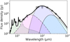 |
Fig. 6 Global SED of the whole region of RCW 36 obtained from the aperture radius of 25′ at the center position of RA = 8:59:30.963, Dec = −43:46:56.270 (J2000.0). To obtain the eight-free parameters, the SED fitting was performed for the original seven-band data plus IRAS 25 μm, 60 μm, and 100 μm data. The thick solid line shows the best-fitting model, which is described in Eq. (1). The very cold dust, cold dust, warm dust, and PAH components are denoted by thin solid, dashed, dash-dotted, and dotted lines, respectively. |
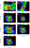 |
Fig. 7 Spatial distributions of (a) cold dust temperature (Tc), (b) very colddust luminosity (Lvc), (c) cold dustluminosity (Lc), (d) warm dust luminosity (Lw), (e) PAH luminosity (LPAH), and (f) far-IR luminosity (LFIR = Lvc + Lc + Lw). The panel g is same asthe panel f, but the positions of seven clumps and OB stars are denoted by circles and crosses, respectively (Ellerbroek et al. 2013; Minier et al. 2013). Dust temperature and luminosity are in units of kelvin and solar luminosity, respectively. For each luminosity map, the colour scale ranges from 2 to 98% of the peak luminosity. The contours superimposed on the images are the same as those in Fig. 2. |
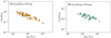 |
Fig. 8 Correlation plots of (a) L[CII]∕LFIR vs. LFIR and (b) L[CII]∕LPAH vs. LPAH. |
4.2 Variations of L[C II]/LFIR and L[C II]/LPAH
In Fig. 8, L[C II]∕LFIR varies about one order of magnitude, while L[C II]∕LPAH shows a smaller variation. Such large variation in L[C II]∕LFIR is also observed in the Milky Way and nearby galaxies (e.g. Wright et al. 1991; Stacey et al. 1991; Malhotra et al. 2001; Croxall et al. 2012; Kramer et al. 2013; Goicoechea et al. 2015; Smith et al. 2017). According to Goicoechea et al. (2015), the large variation observed toward the Orion molecular cloud 1 (OMC1) can be explained by those in the total dust-cloud column relative to the [C II]-emitting column along each line of sight (geometry effect). To verify whether such geometry effects can also be the cause of the broad range of L[C II]∕LFIR in RCW 36, the dust opacity close to the [C II] 158 μm line is calculated as  for an optically thin condition, where Ωpix is the solid angle subtended by each pixel (90′′). Figure 9 shows L[C II]∕LFIR as a function of τd,160, colour-coded according to Tc. The dashed line corresponds to the relation calculated from a simple face-on slab model assuming a uniform dust temperature:
 ![Mathematical equation: $L_{\mathrm{[\ion{C}{ii}]}}/L_{\mathrm{FIR}}\,{=}\, C(1-e^{-\tau_{\mathrm{d,160}}})^{-1}\simeq C\tau_{\mathrm{d,160}}^{-1}$](/articles/aa/full_html/2021/07/aa35739-19/aa35739-19-eq7.png) (see Fig. 16a in Goicoechea et al. 2015), where C is a constant determined so that the model curve intercepts the median L[C II]∕LFIR and τd,160 values. Clearly, the measured data are distributed along the model line because of small variation in the cold dust temperature. Therefore, large variations inL[C II]∕LFIR toward RCW 36 are explained by the geometry effect, as in the case of OMC1.
(see Fig. 16a in Goicoechea et al. 2015), where C is a constant determined so that the model curve intercepts the median L[C II]∕LFIR and τd,160 values. Clearly, the measured data are distributed along the model line because of small variation in the cold dust temperature. Therefore, large variations inL[C II]∕LFIR toward RCW 36 are explained by the geometry effect, as in the case of OMC1.
From the spatial correlation analysis among [C II], PAH, warm, cold and very cold dust emissions, [C II] and PAH emissions are spatially in good agreement with each other and thus are considered to mainly arise from the far-UV illuminated face of clouds. As a result, significant variation in L[C II]∕LPAH is not expected from the geometry effect. Thus, another factor seems to affect the observed L[C II]∕LPAH variation. Insuch far-UV dominated regions (PDRs), PAHs are expected to play a significant role of photo-electric heating of gas (Bakes & Tielens 1994). However, its heating efficiency is decreased as the far-UV radiation field increases due to the presence of larger amount of ionised PAHs (Okada et al. 2013). To verify if photo-electric heating efficiency can explain the observed variation of L[C II]∕LPAH, we calculated the intensity of the incident far-UV radiation field G0 in Habing units by using the following equation (Hollenbach & Tielens 1999): G0 ~ IFIR∕2.6 × 10⁻⁴ erg sec−1 cm−2 sr−1, where IFIR is the far-IR intensity obtained from LFIR at each pixel. G0 values thus obtained show the range of ~ 102–104; the peak G0 in RCW36 is six times lower than that in RCW 38 (Kaneda et al. 2013). As expected, L[C II]∕LPAH decreases as G0 increases asshown in Fig. 10. Based on this measured variation of G0 across RCW 36, we explored the range of values of charging parameter which is relevant for photo-electric heating efficiency. We estimated the charging parameter  , where Tg and ne are the gas temperature and the electron density in PDRs. The electron density is calculated from the following equation with assumptionsthat (a) the electrons in PDRs are all provided by ionised carbons and the carbon atoms are fully ionised (ne = 1.6 × 10⁻⁴nH, Sofia et al. 2004) and (b) pressure between H II regions and PDRs is balanced (2ne,H IITe,H II ≃ nHTg);
 (2)
(2)
where nH, ne,H II, and Te,H II are hydrogen gas density in PDRs, electron density, and electron
temperature in H II regions, respectively. Moreover, ne,H II(G0) is derived bysolving G0 at a distance equal to the Strömgren sphere radius and by assuming the fraction of luminosity above 6 eV equal to unity (Tielens 2005) as
 (3)
(3)
where NLyc and L⋆ are the total number of ionising photons by a star and the stellar luminosity, respectively. When we apply NLyc = 1048 photons sec−1 for the spectral type of O9 as the dominant exciting star (Binder & Povich 2018), L⋆ = 8 × 10⁴ L⊙ (Thompson 1984), Te,H II = 7600 K (Shaver & Goss 1970), and measured G0 values, γ ranges from ~ 103 to 105  for typical Tg of 102 –103 K in PDRs (Kaufman et al. 1999). The obtained γ range meets the transition where the charge state of PAHs changes from neutral to fully ionised states (Okada et al. 2013). Therefore, the L[C II]∕LPAH variation can be explained by the variation of the photo-electric heating efficiency on PAHs.
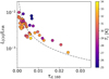 |
Fig. 9 Correlation plot of L[C II]∕LFIR vs. τd,160. The dashed line shows the relation with the model of a simple face-on slab of dust with the [C II] foreground emission (Goicoechea et al. 2015). |
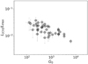 |
Fig. 10 Correlation plot of L[C II]∕LPAH vs. G0. |
4.3 Enhanced brightness ratio of [CII]/160 μm
In Fig. 4, [C II]/160 μm values for RCW 36 are systematically higher than those for RCW 38, while [C II]/9 μm values for RCW 36 are in good agreement with those for RCW 38. Those results indicate that the PAH emission relative to the large-grain emission in RCW 36 is higher than that in RCW 38: difference in SEDs between RCW 36 and RCW 38.
From the previous two sections, results of pixel-by-pixel correlation analyses for RCW 36 suggest that the 160 μm emission traces the column density of dust grains in overall clouds along the line of sight, while [C II] and PAH emissions mainly arise from the far-UV illuminated surface of clouds. RCW 36 is formed in a filamentary molecular cloud with H2 column densities ( ) of ~ 1022–1023 cm−2 (Hill et al. 2011). On the outside (east-west side) of the filament,
  is rapidly dropped to ~ 1021 cm−2: low-column density areas of cold gas and dust grains. In this scenario, the [C II] map shows that PDRs are formed not only in the filament but also in low-column density areas because of the bipolar outflow. Therefore, as shown in Fig. 11, higher values of L[C II]∕LFIR and LPAH∕LFIR are observed in low-column density areas (τd,160 ⪅ 5 × 10⁻²) rather than in the filament.
Based on the picture of the geometry effect, the overall difference in [C II]/160 μm between RCW 36 and RCW 38 can be explained by the difference in the total dust-cloud column relative to the [C II] emitting column. Far-UV photons from massive stars in a filamentary molecular cloud, such as RCW 36, are likely toleak into low-dust column density regions perpendicular to the filament, while those in a clumpy molecular cloud, as in the case of RCW 38, are less likely because stars are surrounded by high-dust column density regions (Wolk et al. 2006; Kaneda et al. 2013; Fukui et al. 2016). In such low-dust column density regions, the [CII] emitting layer is considered to be dominated. Therefore, the enhanced brightness ratio of [C II]/160 μm suggests that RCW36 is dominated by far-UV illuminated cloud surfaces (diffuse PDRs), as compared with RCW38.
5 Conclusions
Large-area [C II] 158 μm mapping of RCW 36 was conducted to investigate properties of [C II] emission influenced by a radiative feedback from massive stars formed in the dense filamentary cloud. The [C II] emission overall extends toward the east-west direction from the peak, which is almost perpendicular to the direction of the cold dense filament. There are two prominent arms extending from the [C II] peak to the north-east and south-west directions, which are spatially in good agreement with shell-like structures of the bipolar lobe clearly seen in the cold dust (Td ~ 30 K) and PAH emissions. From a pixel-by-pixel correlation analysis, the [C II] emission spatially correlates with PAH and cold dust emissions. Therefore, the observed [C II] emission dominantly comes from PDRs. Moreover, we found that the brightness ratio of [C II]/160 μm for RCW 36 is systematically higher than that for RCW 38, while that of [C II]/9 μm for RCW 36 is consistent with RCW 38. The L[C II]∕LFIR ratio shows a large variation (10−2–10−3) as compared with the L[C II]/LPAH ratio. Given the fact that the tight correlation between L[C II]∕LFIR and τd,160, the large variation in L[C II]∕LFIR can be explained by that in the total dust-cloud column relative to the [C II] and PAHs emitting column along each line of sight (geometry effect). Based on the picture of the geometry effect, the enhanced brightness ratio of [C II]/160 μm is attributedto the difference in gas structures where massive stars are formed; unlike RCW 38 where massive stars are formed inside a clumpy molecular cloud, RCW 36 is formed in a filamentary molecular cloud and is then dominated by far-UV illuminated cloud surfaces. Thus, the difference in large-scale gas structures is shown to be the cause of the enhanced brightness ratio of [C II]/160 μm.
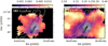 |
Fig. 11 Luminosity ratio maps of (a) L[C II]∕LFIR and (b) LPAH∕LFIR obtained from Fig. 7. The Lvc contours superimposed on the images are linearly spaced among ten levels from 0.95 to 9.5 L⊙. |
Acknowledgements
We greatly appreciate all the members of the Infrared Astronomy Group of TIFR and the staff members of the TIFRBalloon Facility in Hyderabad, India, for their support during balloon flights. We acknowledge support of the Department of Atomic Energy, Government of India, under project no. 12-R&D-TFR-5.02-0200. The authors gratefully acknowledgethe contribution of the anonymous referee’s comments in improving our manuscript and also thank Dr. Sano for providing contours of CO data. This research was supported by JSPS KAKENHI Grant Number 25247020 and 18H01252. Part of this work is based on observations with AKARI, a JAXA project with the participation of ESA. PACS has been developed by a consortium of institutes led by MPE (Germany) and including UVIE (Austria); KU Leuven, CSL, IMEC (Belgium); CEA, LAM (France); MPIA (Germany); INAF-IFSI/OAA/OAP/OAT, LENS, SISSA (Italy); IAC (Spain). This development has been supported by the funding agencies BMVIT (Austria), ESA-PRODEX (Belgium), CEA/CNES (France), DLR (Germany), ASI/INAF (Italy), and CICYT/MCYT (Spain). SPIRE has been developed by a consortium of institutes led by Cardiff University (UK) and including Univ. Lethbridge (Canada); NAOC (China); CEA, LAM (France); IFSI, Univ. Padua (Italy); IAC (Spain); Stockholm Observatory(Sweden); Imperial College London, RAL, UCL-MSSL, UKATC, Univ. Sussex (UK); and Caltech, JPL, NHSC, Univ. Colorado (USA). This development has been supported by national funding agencies: CSA (Canada); NAOC (China); CEA, CNES, CNRS (France); ASI (Italy); MCINN (Spain); SNSB (Sweden); STFC, UKSA (UK); and NASA (USA). This research is supported by JSPS KAKENHI Grant Numbers JP25247020, JP18H01252.
References
- Anderson, L. D., Zavagno, A., Deharveng, L., et al. 2012, A&A, 542, A10 [NASA ADS] [CrossRef] [EDP Sciences] [Google Scholar]
- André, P., Men’shchikov, A., Bontemps, S., et al. 2010, A&A, 518, L102 [NASA ADS] [CrossRef] [EDP Sciences] [Google Scholar]
- Aniano, G., Draine, B. T., Gordon, K. D., & Sandstrom, K. 2011, PASP, 123, 1218 [NASA ADS] [CrossRef] [Google Scholar]
- Bakes, E. L. O., & Tielens, A. G. G. M. 1994, ApJ, 427, 822 [NASA ADS] [CrossRef] [Google Scholar]
- Baug, T., Ojha, D. K., Dewangan, L. K., et al. 2015, MNRAS, 454, 4335 [NASA ADS] [CrossRef] [Google Scholar]
- Binder, B. A., & Povich, M. S. 2018, ApJ, 864, 136 [NASA ADS] [CrossRef] [Google Scholar]
- Bohlin, R. C., Savage, B. D., & Drake, J. F. 1978, ApJ, 224, 132 [NASA ADS] [CrossRef] [Google Scholar]
- Casey, C. M. 2012, MNRAS, 425, 3094 [Google Scholar]
- Croxall, K. V., Smith, J. D., Wolfire, M. G., et al. 2012, ApJ, 747, 81 [NASA ADS] [CrossRef] [Google Scholar]
- Dewangan, L. K., Baug, T., Ojha, D. K., et al. 2017a, ApJ, 845, 34 [NASA ADS] [CrossRef] [Google Scholar]
- Dewangan, L. K., Ojha, D. K., & Zinchenko, I. 2017b, ApJ, 851, 140 [CrossRef] [Google Scholar]
- Draine, B. T., & Li, A. 2007, ApJ, 657, 810 [Google Scholar]
- Ellerbroek, L. E., Bik, A., Kaper, L., et al. 2013, A&A, 558, A102 [NASA ADS] [CrossRef] [EDP Sciences] [Google Scholar]
- Fukui, Y., Torii, K., Ohama, A., et al. 2016, ApJ, 820, 26 [Google Scholar]
- Gaia Collaboration (Brown, A. G. A., et al.) 2018, A&A, 616, A1 [NASA ADS] [CrossRef] [EDP Sciences] [Google Scholar]
- Ghosh, S. K., Iyengar, K. V. K., Rengarajan, T. N., et al. 1988, ApJ, 330, 928 [NASA ADS] [CrossRef] [Google Scholar]
- Glass, I. S. 1999, Handbook of Infrared Astronomy (Cambridge: Cambridge University Press) [CrossRef] [Google Scholar]
- Goicoechea, J. R., Teyssier, D., Etxaluze, M., et al. 2015, ApJ, 812, 75 [NASA ADS] [CrossRef] [Google Scholar]
- Hill, T., Motte, F., Didelon, P., et al. 2011, A&A, 533, A94 [NASA ADS] [CrossRef] [EDP Sciences] [Google Scholar]
- Hollenbach, D. J., & Tielens, A. G. G. M. 1999, Rev. Mod. Phys., 71, 173 [Google Scholar]
- Ishihara, D., Onaka, T., Kataza, H., et al. 2010, A&A, 514, A1 [NASA ADS] [CrossRef] [EDP Sciences] [Google Scholar]
- Jaffe, D. T., Zhou, S., Howe, J. E., et al. 1994, ApJ, 436, 203 [NASA ADS] [CrossRef] [Google Scholar]
- Kaneda, H., Nakagawa, T., Ghosh, S. K., et al. 2013, A&A, 556, A92 [CrossRef] [EDP Sciences] [Google Scholar]
- Kaufman, M. J., Wolfire, M. G., Hollenbach, D. J., & Luhman, M. L. 1999, ApJ, 527, 795 [Google Scholar]
- Kramer, C., Abreu-Vicente, J., García-Burillo, S., et al. 2013, A&A, 553, A114 [NASA ADS] [CrossRef] [EDP Sciences] [Google Scholar]
- Li, A., & Draine, B. T. 2001, ApJ, 554, 778 [Google Scholar]
- Malhotra, S., Kaufman, M. J., Hollenbach, D., et al. 2001, ApJ, 561, 766 [Google Scholar]
- Minier, V., Tremblin, P., Hill, T., et al. 2013, A&A, 550, A50 [NASA ADS] [CrossRef] [EDP Sciences] [Google Scholar]
- Molinari, S., Swinyard, B., Bally, J., et al. 2010, A&A, 518, L100 [NASA ADS] [CrossRef] [EDP Sciences] [Google Scholar]
- Mookerjea, B., Ghosh, S. K., Kaneda, H., et al. 2003, A&A, 404, 569 [NASA ADS] [CrossRef] [EDP Sciences] [Google Scholar]
- Myers, P. C. 2009, ApJ, 700, 1609 [NASA ADS] [CrossRef] [EDP Sciences] [Google Scholar]
- Nakagawa, T., Yui, Y. Y., Doi, Y., et al. 1998, ApJS, 115, 259 [NASA ADS] [CrossRef] [Google Scholar]
- Okada, Y., Pilleri, P., Berné, O., et al. 2013, A&A, 553, A2 [NASA ADS] [CrossRef] [EDP Sciences] [Google Scholar]
- Onaka, T., Matsuhara, H., Wada, T., et al. 2007, PASJ, 59, 401 [NASA ADS] [Google Scholar]
- Sano, H., Enokiya, R., Hayashi, K., et al. 2018, PASJ, 70, S43 [NASA ADS] [CrossRef] [Google Scholar]
- Seabold, S., & Perktold, J. 2010, in 9th Python in Science Conference [Google Scholar]
- Shaver, P. A., & Goss, W. M. 1970, Aust. J. Phys. Astrophys. Suppl., 14, 133 [NASA ADS] [Google Scholar]
- Smith, J. D. T., Croxall, K., Draine, B., et al. 2017, ApJ, 834, 5 [NASA ADS] [CrossRef] [Google Scholar]
- Sofia, U. J., Wolff, M. J., Rachford, B., et al. 2004, AAS Meeting Abs., 205, 59.16 [Google Scholar]
- Stacey, G. J., Geis, N., Genzel, R., et al. 1991, ApJ, 373, 423 [NASA ADS] [CrossRef] [Google Scholar]
- Suzuki, T., Kaneda, H., Onaka, T., Nakagawa, T., & Shibai, H. 2010, A&A, 521, A48+ [Google Scholar]
- Thompson, R. I. 1984, ApJ, 283, 165 [Google Scholar]
- Tielens, A. G. G. M. 2005, The Physics and Chemistry of the Interstellar Medium (Cambridge: Cambridge University Press) [CrossRef] [Google Scholar]
- Wolk, S. J., Spitzbart, B. D., Bourke, T. L., & Alves, J. 2006, AJ, 132, 1100 [NASA ADS] [CrossRef] [Google Scholar]
- Wright, E. L., Mather, J. C., Bennett, C. L., et al. 1991, ApJ, 381, 200 [NASA ADS] [CrossRef] [Google Scholar]
- Xue, M., Jiang, B. W., Gao, J., et al. 2016, ApJS, 224, 23 [NASA ADS] [CrossRef] [Google Scholar]
- Zinnecker, H., & Yorke, H. W. 2007, ARA&A, 45, 481 [NASA ADS] [CrossRef] [Google Scholar]
All Figures
|
Fig. 1 [C II] observation area (solid box) of RCW 36 superimposed on a composite image shown with the equatorial J2000 coordinate system: AKARI 9 μm (blue), Herschel 70 μm (green), and Herschel 250 μm (red). RCW 36 is formed in a large-scale filament extending north-south direction. A bipolar lobe, shell-like structures and a ring-like structure (black dashed ellipse) are identified by Minier et al. (2013). |
| In the text | |
|
Fig. 2 [C II] intensity map of RCW 36 showing an area of 20′ × 15′ taken by FPS100. The contours are linearly spaced 12 levels from 3.3 × 10⁻⁴ to 1.9 × 10⁻³ erg sec−1 cm−2 sr−1. The PSF size in FWHM is shown in the lower-left corner. |
| In the text | |
|
Fig. 3 Seven-band images of RCW 36 from the AKARI and Herschel data in (a) AKARI 9 μm, (b) AKARI 18 μm, (c) Herschel 70 μm, (d) Herschel 160 μm, (e) Herschel 250 μm, (f) Herschel 350 μm, and (g) Herschel 500 μm bands. In each image, the colour bar is given in units of MJy sr−1. The PSF size in FWHM is in the lower left corner. The contours superimposed on the images are the same as those in Fig. 2. |
| In the text | |
|
Fig. 4 Correlation plots of brightness between (a) [C II] and 9 μm, and (b) [C II]and 160 μm for RCW 36 (circle), together with those for RCW 38 (square) from Fig. 3 in Kaneda et al. (2013). |
| In the text | |
|
Fig. 5 Same as Fig. 2, but 12CO(J = 2–1) contours (Fig. 4a in Sano et al. 2018) and positions of OB stars (cross) (Ellerbroek et al. 2013). The cyan and red coloured contours represent two-velocity molecular cloud components with VLSR = 4.1–6.1 km s−1 (blue cloud) and 7.6–12.0 km s−1 (red cloud), respectively. The spatial resolution of the 12CO(J = 2–1) map taken by NANTEN2 is similar to the [C II] map (90′′). |
| In the text | |
|
Fig. 6 Global SED of the whole region of RCW 36 obtained from the aperture radius of 25′ at the center position of RA = 8:59:30.963, Dec = −43:46:56.270 (J2000.0). To obtain the eight-free parameters, the SED fitting was performed for the original seven-band data plus IRAS 25 μm, 60 μm, and 100 μm data. The thick solid line shows the best-fitting model, which is described in Eq. (1). The very cold dust, cold dust, warm dust, and PAH components are denoted by thin solid, dashed, dash-dotted, and dotted lines, respectively. |
| In the text | |
|
Fig. 7 Spatial distributions of (a) cold dust temperature (Tc), (b) very colddust luminosity (Lvc), (c) cold dustluminosity (Lc), (d) warm dust luminosity (Lw), (e) PAH luminosity (LPAH), and (f) far-IR luminosity (LFIR = Lvc + Lc + Lw). The panel g is same asthe panel f, but the positions of seven clumps and OB stars are denoted by circles and crosses, respectively (Ellerbroek et al. 2013; Minier et al. 2013). Dust temperature and luminosity are in units of kelvin and solar luminosity, respectively. For each luminosity map, the colour scale ranges from 2 to 98% of the peak luminosity. The contours superimposed on the images are the same as those in Fig. 2. |
| In the text | |
|
Fig. 8 Correlation plots of (a) L[CII]∕LFIR vs. LFIR and (b) L[CII]∕LPAH vs. LPAH. |
| In the text | |
|
Fig. 9 Correlation plot of L[C II]∕LFIR vs. τd,160. The dashed line shows the relation with the model of a simple face-on slab of dust with the [C II] foreground emission (Goicoechea et al. 2015). |
| In the text | |
|
Fig. 10 Correlation plot of L[C II]∕LPAH vs. G0. |
| In the text | |
|
Fig. 11 Luminosity ratio maps of (a) L[C II]∕LFIR and (b) LPAH∕LFIR obtained from Fig. 7. The Lvc contours superimposed on the images are linearly spaced among ten levels from 0.95 to 9.5 L⊙. |
| In the text | |
Current usage metrics show cumulative count of Article Views (full-text article views including HTML views, PDF and ePub downloads, according to the available data) and Abstracts Views on Vision4Press platform.
Data correspond to usage on the plateform after 2015. The current usage metrics is available 48-96 hours after online publication and is updated daily on week days.
Initial download of the metrics may take a while.