| Issue |
A&A
Volume 650, June 2021
|
|
|---|---|---|
| Article Number | L14 | |
| Number of page(s) | 8 | |
| Section | Letters to the Editor | |
| DOI | https://doi.org/10.1051/0004-6361/202141297 | |
| Published online | 23 June 2021 | |
Letter to the Editor
The sulphur saga in TMC-1: Discovery of HCSCN and HCSCCH⋆
1
Grupo de Astrofísica Molecular, Instituto de Física Fundamental (IFF-CSIC), C/ Serrano 121, 28006 Madrid, Spain
e-mail: This email address is being protected from spambots. You need JavaScript enabled to view it.
, This email address is being protected from spambots. You need JavaScript enabled to view it.
2
Department of Applied Chemistry, Science Building II, National Yang Ming Chiao Tung University, 1001 Ta-Hsueh Rd., Hsinchu 30010, Taiwan
3
Centro de Desarrollos Tecnológicos, Observatorio de Yebes (IGN), 19141 Yebes, Guadalajara, Spain
4
Observatorio Astronómico Nacional (IGN), C/Alfonso XII, 3, 28014 Madrid, Spain
Received:
12
May
2021
Accepted:
21
May
2021
Abstract
We report the detection, for the first time in space, of cyano thioformaldehyde (HCSCN) and propynethial (HCSCCH) towards the starless core TMC-1. Cyano thioformaldehyde presents a series of prominent a- and b-type lines, which are the strongest previously unassigned features in our Q-band line survey of TMC-1. Remarkably, HCSCN is four times more abundant than cyano formaldehyde (HCOCN). On the other hand, HCSCCH is five times less abundant than propynal (HCOCCH). Surprisingly, we find an abundance ratio HCSCCH/HCSCN of ∼0.25, in contrast with most other ethynyl-cyanide pairs of molecules for which the CCH-bearing species is more abundant than the CN-bearing one. We discuss the formation of these molecules in terms of neutral-neutral reactions of S atoms with CH2CCH and CH2CN radicals as well as of CCH and CN radicals with H2CS. The calculated abundances for the sulphur-bearing species are, however, significantly below the observed values, which points to an underestimation of the abundance of atomic sulphur in the model or to missing formation reactions, such as ion-neutral reactions.
Key words: molecular data / line: identification / ISM: molecules / ISM: individual objects: TMC-1 / astrochemistry
Based on observations carried out with the Yebes 40 m telescope (projects 19A003, 20A014, 20D023, and 21A011). The 40 m radio telescope at Yebes Observatory is operated by the Spanish Geographic Institute, (IGN, Ministerio de Transportes, Movilidad y Agenda Urbana).
© ESO 2021
1. Introduction
The chemistry of sulphur-bearing molecules in cold interstellar clouds is an active area of research (Vidal et al. 2017; Cernicharo et al. 2021a,b). Recently, Cernicharo et al. (2021b) reported the detection of five new sulphur-bearing species in TMC-1, a source that presents an interesting carbon-rich chemistry that leads to the formation of long neutral carbon chain radicals and their anions, cyanopolyynes (see Cernicharo et al. 2020a,b and references therein), pure hydrocarbon cycles, and polycyclic aromatic hydrocarbons (Cernicharo et al. 2021c; Burkhardt et al. 2021; McCarthy et al. 2021). A large variety of S-bearing molecules are also present in this source, which leads to new questions regarding the formation routes to these species. It is clear that many ion-neutral and neutral-neutral reactions involving S-bearing species have to be studied to improve the reliability of chemical models (Petrie 1996; Bulut et al. 2021). Unveiling new sulphur-bearing species can also help to understand the chemistry of sulphur by comparing the observed abundances with those predicted by chemical models.
In this Letter we report the discovery of two new sulphur-bearing molecules: HCSCN (cyano thioformaldehyde) and HCSCCH (propynethial). Figure 1 shows the structure of these molecules. The derived abundances are compared with the oxygen analogues of these species, HCOCN (cyano formaldehyde) and HCOCCH (propynal). We discuss plausible reactions that could lead to the formation of these species with the aid of a chemical model.
 |
Fig. 1. Structure of cyano thioformaldehyde, HCSCN, and ethynyl thioformaldehyde, HCSCCH, also known as propynethial. |
2. Observations
New receivers, built within the Nanocosmos project1 and installed at the Yebes 40 m radio telescope, were used for the observations of TMC-1. A detailed description of the system is given by Tercero et al. (2021). The Q-band receiver consists of two high electron mobility transistor cold amplifiers covering the 31.0–50.3 GHz band with horizontal and vertical polarisations. The backends are 2 × 8 × 2.5 GHz fast Fourier transform (FT) spectrometers with a spectral resolution of 38.15 kHz that provide the whole coverage of the Q-band in both polarisations. The main beam efficiency varies from 0.6 at 32 GHz to 0.43 at 50 GHz.
The line survey of TMC-1 (αJ2000 = 4h41m41.9s and δJ2000 = +25 ° 41′27.0″) in the Q-band was performed in several sessions. The first results (Cernicharo et al. 2020a,b) were based on two observing runs performed in November 2019 and February 2020. Two different frequency coverages were achieved, 31.08–49.52 GHz and 31.98–50.42 GHz, in order to check that no spurious spectral ghosts are produced in the down-conversion chain. Additional data were taken in October 2020, December 2020, and January–April 2021. The observing procedure was frequency switching with a frequency throw of 10 MHz for the two first runs and of 8 MHz for all the others. Receiver temperatures in the runs achieved in 2020 vary from 22 K at 32 GHz to 42 K at 50 GHz. Some power adaptation in the down-conversion chains reduced the receiver temperatures in 2021 to 16 K at 32 GHz and 25 K at 50 GHz. The sensitivity of the survey varies along the Q-band between 0.25 and 1 mK, which is a considerable improvement over previous line surveys in the 31–50 GHz frequency range (Kaifu et al. 2004). The acronym we have assigned to this line survey is QUIJOTE (Q-band Ultrasensitive Inspection Journey to the Obscure Tmc-1 Environment).
The intensity scale used in this work, the antenna temperature ( ), was calibrated using two absorbers at different temperatures and the atmospheric transmission model ATM (Cernicharo 1985; Pardo et al. 2001). Calibration uncertainties of 10% were adopted. All data were analysed using the GILDAS package2.
3. Assignment of unidentified lines to HCSCN
Our millikelvin-sensitive line survey of TMC-1 has revealed hundreds of unknown features whose identification challenges our state-of-the-art understanding of the chemistry of this object (Cernicharo et al. 2021b,c). Line identification in this work was done using the catalogues MADEX (Cernicharo 2012), CDMS (Müller et al. 2005), and JPL (Pickett et al. 1998).
One surprising result in our data is the presence of a few strong unknown features with intensities around 10 mK. Three of them are in an excellent harmonic relation of 6:7:8. A fit to the standard Hamiltonian of a linear molecule provides a rotational constant, B, of 3082.8334 ± 0.0029 MHz and a distortion constant, D, of 40.890 ± 0.027 kHz. Such a large distortion constant points towards an asymmetric rotor. Hence, these three lines could correspond to the transitions Ka = 0 of Jup = 6, 7, and 8 of a molecule with (B + C)/2 = 3082.8 MHz. This suggests that the molecule could have a total of either four or five N, C, and/or O atoms. We explored around these features, looking for the Ka = 1 lines. After some iterative work, we found six of these lines that can be fitted with a reduced number of rotational and distortion constants for a total of nine transitions. These lines are shown in Fig. 2. The assigned quantum numbers correspond to a-type transitions. The carrier is definitely an asymmetric rotor. Hence, we could expect to have b-type transitions if the molecule has a large μb. From the rotational and distortion constants derived from the a-type transitions, we predicted the spectrum for b-type transitions and found nine of them, as shown in Fig. 3. Moreover, these b-type transitions show a series of lines around the predicted frequencies, which is reminiscent of the hyperfine structure of an N-nucleus. Assuming this is the case, we fitted all these lines and obtained the rotational constants provided in Table 1. The derived values for χaa and χbb definitively correspond to a CN group. The hyperfine structure of the a-type transitions is not resolved with our spectral resolution. Hence, the three strongest components appear as a single feature. No c-type transitions were found at the level of sensitivity of our survey.
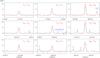 |
Fig. 2. Selected a-type transitions of HCSCN. The abscissa corresponds to the rest frequency of the lines assuming a local standard of rest velocity of the source of 5.83 km s−1. Frequencies and intensities for the observed lines are given in Table A.1. The ordinate is the antenna temperature, corrected for atmospheric and telescope losses, in millikelvin. The quantum numbers for each transition are indicated in the upper left corner of the corresponding panel. The red lines show the computed synthetic spectrum for this species for Tr = 5 K and a column density of 1.3 × 1012 cm−2. Blanked channels correspond to negative features produced in the folding of the frequency switching data. |
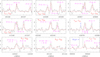 |
Fig. 3. Same as Fig. 2 but for the b-type transitions of HCSCN. The red lines show the computed synthetic spectrum for this species for Tr = 5 K and a column density of 1.3 × 1012 cm−2. |
Spectroscopic parameters for HCSCN, HC34SCN, and HCSCCH.
3.1. Identifying the carrier: Laboratory microwave spectroscopy experiments
We explored, using ab initio calculations, a significant number of the combinations of HxCyNz and HxCyOz without finding a good agreement with the constants of our new species. Molecules such as bent-HC4N and c-C3HCN have rotational constants close, within 10%, to ours. Several years ago we implemented a species in MADEX that matches our constants rather well. It is HCSCN (see Table 1), and it was observed in the laboratory by Bogey et al. (1989). Another species with very close constants to ours (see Table 1), HCSCCH, is also implemented in MADEX, and we found several of its lines in our data (see Sect. 4). Hence, HCSCN could be a good candidate for TMC-1. Unfortunately, with the rotational constants provided by Bogey et al. (1989), the species is not detected. We explored the literature for additional laboratory data for HCSCN and found a contribution to the Ohio State 67th International Symposium on Molecular Spectroscopy (Zaleski et al. 2012). In the presentation, the reported rotational constants for HCSCN agree perfectly with those derived in TMC-1 (see Table 1); Zaleski et al. (2012) also claim a difference between their data and those of Bogey et al. (1989). The detection of HCSCCH, and the good agreement between the TMC-1 constants and those of Zaleski et al. (2012), points to an uncorrect assignment of the HCSCN lines in the Bogey et al. (1989) work. A detailed search for a publication of Zaleski et al. data in a refereed journal has, regrettably, been unsuccessful.
In order to confirm that the carrier of our prominent unknown features in TMC-1 is indeed HCSCN, we performed laboratory measurements. The rotational spectrum of HCSCN was measured by a Balle-Flygare-type FT microwave spectrometer combined with a pulsed discharge nozzle (Endo et al. 1994; Cabezas et al. 2016). HCSCN was produced in a supersonic expansion by a pulsed electric discharge of a gas mixture of CH3CN (0.2%) and CS2 (0.2%) diluted in Ar and by applying a voltage of 2.0 kV through the throat of the nozzle source. We observed a total of nine a-type and two b-type transitions (see Fig. ) at the predicted frequencies using the TMC-1 observed lines. To confirm the identity of the spectral carrier, we observed the HC34SCN isotopic species in their natural abundance. Their rotational transitions (see Fig. ) appear exactly at the expected frequencies considering the isotopic shift for 34S. All the observed lines for HCSCN and HC34SCN are shown in Tables B.1 and B.2.
We performed ab initio calculations at the MP2/6-311++G(d,p) level of theory to optimise the HCSCN molecular structure and calculate the electric dipole moment components. We obtained μa and μb values of 2.03 and 1.69 D. Details of these calculations are given in Appendix B. Our calculations also indicate that the observed rotational transitions reported by Bogey et al. (1989) correspond to the lowest excited vibrational state of HCSCN, ν9, which lies at 198.1 cm−1 above the ground vibrational state.
The merged fit to the TMC-1 frequencies and the fit to our laboratory measurements provide a set of rotational constants (see Table 1) that can be used to predict the frequencies of HCSCN up to 100 GHz with calculated uncertainties below 50 kHz for Ka = 0 and 1. Within the present sensitivity of our survey, no lines of HC34SCN, which are expected to be 20 times weaker than those of HCSCN, were found.
3.2. Column density of HCSCN
We used a model fitting technique (see Cernicharo et al. 2021a) in which the rotational temperature, the column density, and the μa/μb ratio are varied. A uniform brightness temperature source with a diameter of 80″ was assumed (Fossé et al. 2001). The best fit provides a rotational temperature of 5.0 ± 0.5 K, a dipole moment component ratio, μa/μb, of 0.70 ± 0.05, and a column density of (6.2 ± 0.5)/ cm−2, where μa is the component of the dipole moment along the a-axis of the molecule. Adopting the value of the total dipole moment derived by our ab initio calculations and the μa/μb ratio of 0.7 obtained from our observations, we derive μa = 2.16 D. Hence, the column density of HCSCN is (1.3 ± 0.1)×1012 cm−2. Adopting a column density of H2 of 1022 cm−2 for TMC-1 (Cernicharo & Guélin 1987), the abundance of HCSCN relative to H2 is 1.3 × 10⁻¹⁰.
The column density of cyano formaldehyde, HCOCN, in TMC-1 is (3.5 ± 0.5)×1011 cm−2(see Appendix ). Hence, the abundance ratio HCSCN/HCOCN is ∼4, which is surprising considering that the elemental gas-phase abundance of oxygen is expected to be much larger than that of sulphur. Moreover, the column density of formaldehyde is 5 × 1014 cm−2 (Agúndez & Wakelam 2013), while that of H2CS is 4.7 × 1013 cm−2 (Cernicharo et al. 2021a). Hence, the abundance ratio HCSCN/HCOCN is a factor of 40 larger than that of H2CS/H2CO (∼0.1).
4. Detection of propynethial, HCSCCH
The detection of HCSCN suggests that other derivatives of thioformaldehyde could be present in TMC-1. The obvious candidate is ethynyl thioformaldehyde (HCSCCH), also known as propynethial. This molecule has been observed in the laboratory up to 630 GHz and Jmax = 107 (Brown & Godfrey 1982; Cabtree et al. 2016; Margulès et al. 2020). Its dipole moment components have been measured to be μa = 1.763 D and μb = 0.661 D (Brown & Godfrey 1982). Six lines of this molecule were found in our data, and they are shown in Fig. 4. The lines are considerably weaker than those of HCSCN. We searched for more transitions of this species, but their expected intensity is below the present sensitivity of the survey. Nevertheless, the detection of all the strongest lines of HCSCCH in the Q-band is solid and robust. None of the detected lines is blended with any other feature from known species. This species was searched for towards different sources, including TMC-1, by Margulès et al. (2020) with negative results. However, the transition they searched for towards TMC-1 has an upper energy level of 13.7 K and is predicted to be very weak by our models. Assuming the same source parameters and rotational temperature as for HCSCN, we derive a column density for this species of (3.2 ± 0.4) × 1011 cm−2, which is eight times lower than the upper limit derived by Margulès et al. (2020). Therefore, we obtain an abundance ratio HCSCN/HCSCCH of 4 ± 1. The column density of HCOCCH in this source is (1.5 ± 0.2) × 1012 cm−2 (see Appendix ). Hence, the abundance ratio HCOCCH/HCSCCH is 5 ± 1, which is of the order of the H2CO/H2CS abundance ratio (∼10; see above).
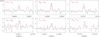 |
Fig. 4. Same as Fig. 2 but for the observed transitions of HCSCCH towards TMC-1. The red line shows the computed synthetic spectrum for propynethial assuming Tr = 5 K and N(HCCCHS) = 3.2 × 1011 cm−2. |
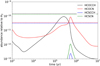 |
Fig. 5. Calculated fractional abundances as a function of time. Observed abundances in TMC-1 are indicated by dashed horizontal lines. |
HCSCCH is an isomer of H2CCCS, a molecule recently found in TMC-1 by Cernicharo et al. (2021b). The column density of the latter has been derived to be (3.7 ± 0.3) × 1011 cm−2. Hence, the abundance ratio between both isomers is ∼1. The energy difference between them is 2 kcal mol−1, the H2CCCS isomer being the more stable one (Cabtree et al. 2016). Finally, we could expect HC4CHS, which could result from the reaction of C4H with H2CS, to be present in TMC-1. Microwave laboratory data for this species are available (McCarthy et al. 2017). We searched for its strongest transitions, but we only derive a 3σ upper limit to its column density of 1012 cm−2.
5. Discussion
The molecules HCSCN and HCSCCH are chemically related as they share an HCS subunit in which the carbon atom is bonded to a CN or a CCH group. Moreover, the oxygen analogues HCOCN and HCOCCH are also chemically related to the two aforementioned molecules since they result from the substitution of the sulphur atom with an oxygen atom. One can therefore conceive of similar chemical routes to these four molecules. A first formation pathway can be provided by
 (1a)
(1a)
 (1b)
(1b)
 (1c)
(1c)
 (1d)
(1d)
These reactions have not been studied, but one could reasonably expect them to be fast at low temperatures. Loison et al. (2016) assume that reaction (1a) is rapid and find that it is the main formation route to HCOCCH in cold interstellar clouds. A second formation route can be provided by
 (2a)
(2a)
 (2b)
(2b)
 (2c)
(2c)
 (2d)
(2d)
Quantum chemical calculations indicate that reaction (2a) could be rapid at low temperatures since the small calculated barrier is within the uncertainty of the calculations (Dong et al. 2005), while reaction (2b) is barrier-less (Tonolo et al. 2020). These authors also suggest that the reaction CN + CH3CHO can plausibly form HCOCN, although it is probably less efficient than reaction (2b) since CH3CHO is about 80 times less abundant than H2CO in TMC-1 (Agúndez & Wakelam 2013).
We implemented the aforementioned neutral-neutral reactions with a rate coefficient of 10−10 cm3 s−1 in a gas-phase chemical model, in which we adopted typical physical conditions of cold dark clouds (see e.g. Agúndez & Wakelam 2013) and used the chemical network UMIST RATE12 (McElroy et al. 2013), revised and expanded according to Loison et al. (2017) and Vidal et al. (2017). The chemical model reproduces the observed abundances of the O-bearing molecules HCOCCH and HCOCN reasonably well. Moreover, the observed abundance ratio HCOCCH/HCOCN of ∼4 is of the same order as the observed abundance ratios CCH/CN (∼10; Pratap et al. 1997) and CH2CCH/CH2CN (∼6; Agúndez et al. 2021; Cabezas et al. 2021), which is consistent with the chemical routes proposed. In the case of the S-bearing molecules HCSCCH and HCSCN, the chemical model underestimates their abundances by two orders of magnitude, which may be related to an excessively low abundance of atomic sulphur calculated by the chemical model or to missing formation reactions, such as ion-neutral reactions.
6. Conclusions
We have reported the discovery of HCSCN and HCSCCH in TMC-1. While HCSCCH is five times less abundant than its oxygen analogue, propynal, we find that HCSCN is four times more abundant than HCOCN. Further studies on plausible formation reactions of HCSCN and HCSCCH are needed.
Acknowledgments
This research has been funded by ERC through grant ERC-2013-Syg-610256-NANOCOSMOS. Authors also thank Ministerio de Ciencia e Innovación (Spain) for funding support through projects AYA2016-75066-C2-1-P, PID2019-106235GB-I00 and PID2019-107115GB-C21/AEI/10.13039/501100011033. MA thanks Ministerio de Ciencia e Innovación for grant RyC-2014-16277. YE thanks Ministry of Science and Technology, Taiwan, for grant No. MOST 108-2113-M-009-025 and MOST 108-2811-M-009-520.
References
- Agúndez, M., & Wakelam, V. 2013, Chem. Rev., 113, 8710 [Google Scholar]
- Agúndez, M., Cabezas, C., Tercero, B., et al. 2021, A&A, 647, L10 [EDP Sciences] [Google Scholar]
- Bogey, M., Demuynck, C., Destombes, J. L., et al. 1989, J. Am. Chem. Soc., 111, 7399 [Google Scholar]
- Bogey, M., Demuynck, C., Destombes, J. L., et al. 1995, J. Mol. Spectrosc., 172, 344 [Google Scholar]
- Brown, R. D., & Godfrey, P. D. 1982, Aust. J. Chem., 35, 1747 [CrossRef] [Google Scholar]
- Bulut, N., Roncero, O., Aguado, A., et al. 2021, A&A, 646, A5 [NASA ADS] [CrossRef] [EDP Sciences] [Google Scholar]
- Burkhardt, A. M., Lee, K. L. K., Changala, P. B., et al. 2021, ApJ, 913, L18 [Google Scholar]
- Cabezas, C., Guillemin, J.-C., & Endo, Y. 2016, J. Chem. Phys., 145, 184304 [Google Scholar]
- Cabezas, C., Endo, Y., Roueff, E., et al. 2021, A&A, 646, L1 [NASA ADS] [CrossRef] [EDP Sciences] [Google Scholar]
- Cabtree, K. N., Martin-Drumel, M.-A., Brown, G. G., et al. 2016, J. Chem. Phys., 144, 124201 [CrossRef] [Google Scholar]
- Cernicharo, J. 1985, Internal IRAM report (Granada: IRAM) [Google Scholar]
- Cernicharo, J. 2012, EAS Publ. Ser., 58, 251 [Google Scholar]
- Cernicharo, J., & Guélin, M. 1987, A&A, 176, 299 [Google Scholar]
- Cernicharo, J., Marcelino, N., Pardo, J. R., et al. 2020a, A&A, 641, L9 [NASA ADS] [CrossRef] [EDP Sciences] [Google Scholar]
- Cernicharo, J., Marcelino, N., Agúndez, M., et al. 2020b, A&A, 642, L8 [NASA ADS] [CrossRef] [EDP Sciences] [Google Scholar]
- Cernicharo, J., Cabezas, C., Endo, Y., et al. 2021a, A&A, 646, L3 [EDP Sciences] [Google Scholar]
- Cernicharo, J., Cabezas, C., Agúndez, M., et al. 2021b, A&A, 648, L3 [EDP Sciences] [Google Scholar]
- Cernicharo, J., Agúndez, M., Cabezas, C., et al. 2021c, A&A, 649, L15 [EDP Sciences] [Google Scholar]
- Császár, A. 1989, Chem. Phys. Lett., 162, 361 [Google Scholar]
- Dong, H., Ding, Y.-H., & Sun, C.-C. 2005, J. Chem. Phys., 122, 204321 [Google Scholar]
- Endo, Y., Kohguchi, H., & Ohshima, Y. 1994, Faraday Discuss., 97, 341 [Google Scholar]
- Frisch, M. J., Pople, J. A., & Binkley, J. S. 1984, J. Chem. Phys., 80, 3265 [NASA ADS] [CrossRef] [Google Scholar]
- Frisch, M. J., Trucks, G. W., Schlegel, H. B., et al. 2016, Gaussian 16, revision A.03 [Google Scholar]
- Fossé, D., Cernicharo, J., Gerin, M., & Cox, P. 2001, ApJ, 552, 168 [Google Scholar]
- Gordy, W., & Cook, R. 1984, Microwave Molecular Spectra, Techniques of Chemistry (New York: Wiley) [Google Scholar]
- Irvine, W. M., Brown, R. D., Cragg, D. M., et al. 1988, ApJ, 335, L89 [NASA ADS] [CrossRef] [Google Scholar]
- Jabri, A., Kolesniková, L., Alonso, E. R., et al. 2020, J. Mol. Spectrosc., 372, 111333 [Google Scholar]
- Kaifu, N., Ohishi, M., Kawaguchi, K., et al. 2004, PASJ, 56, 69 [Google Scholar]
- Loison, J.-C., Agúndez, M., Marcelino, N., et al. 2016, MNRAS, 456, 4101 [Google Scholar]
- Loison, J.-C., Agúndez, M., Wakelam, V., et al. 2017, MNRAS, 470, 4075 [NASA ADS] [CrossRef] [Google Scholar]
- Margulès, L., McGuire, B. A., Evans, C. J., et al. 2020, A&A, 642, A206 [EDP Sciences] [Google Scholar]
- McCarthy, M. C., Zou, L., & Martin-Drumel, M.-A. 2017, J. Chem. Phys., 146, 154301 [Google Scholar]
- McCarthy, M. C., Lee, K. L. K., Loomis, R. A., et al. 2021, Nat. Astron., 5, 176 [Google Scholar]
- McElroy, D., Walsh, C., Markwick, A. J., et al. 2013, A&A, 550, A36 [NASA ADS] [CrossRef] [EDP Sciences] [Google Scholar]
- Møller, C., & Plesset, M. S. 1934, Phys. Rev., 46, 618 [Google Scholar]
- Müller, H. S. P., Schlöder, F., Stutzki, J., & Winnewisser, G. 2005, J. Mol. Struct., 742, 215 [Google Scholar]
- Pardo, J. R., Cernicharo, J., & Serabyn, E. 2001, IEEE Trans. Antennas Propag., 49, 12 [Google Scholar]
- Petrie, S. 1996, MNRAS, 281, 666 [NASA ADS] [Google Scholar]
- Pickett, H. M. 1991, JMoSp, 148, 371 [NASA ADS] [Google Scholar]
- Pickett, H. M., Poynter, R. L., Cohen, E. A., et al. 1998, J. Quant. Spectrosc. Radiat. Trans., 60, 883 [Google Scholar]
- Pratap, P., Dickens, J. E., Snell, R. L., et al. 1997, ApJ, 486, 862 [Google Scholar]
- Remijan, A. J., Hollis, J. M., Lovas, F. J., et al. 2008, ApJ, 675, L85 [Google Scholar]
- Tercero, F., López-Pérez, J. A., Gallego, J. D., et al. 2021, A&A, 645, A37 [EDP Sciences] [Google Scholar]
- Tonolo, F., Lupi, J., Puzzarini, C., & Barone, V. 2020, ApJ, 900, 85 [Google Scholar]
- Vidal, T. H. G., Loison, J.-C., Jaziri, A. Y., et al. 2017, MNRAS, 469, 435 [Google Scholar]
- Watson, J. K. G. 1977, in Vibration Spectra and Structure, ed. J. Durig (Amsterdam: Elsevier), 6, 1 [Google Scholar]
- Zaleski, D. P., Neill, J. L., Muckle, M. T., et al. 2012, The Ohio State 67th International Symposium on Molecular Spectroscopy, June 21st, 2012 [Google Scholar]
Appendix A: Line parameters of the observed transitions of HCSCN and HCSCCH
Line parameters for the different molecules studied in this work were obtained by fitting a Gaussian line profile to the observed data. A window of ±15 km s−1 around the local standard of rest velocity of the source was considered for each transition. The derived line parameters for the two molecular species discovered in this work are given in Table A.1.
Line parameters for the lines of HCSCN and HCSCCH.
Appendix B: Laboratory experiments and quantum chemical calculations for HCSCN
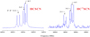 |
Fig. B.1. Fourier transform microwave spectra of HCSCN and HC34SCN showing the 30, 3–20, 2 rotational transition. The spectra show the hyperfine components, labelled with the corresponding values of quantum numbers F′–F′′, clearly resolved. The coaxial arrangement of the adiabatic expansion and the resonator axis produces an instrumental Doppler doubling. The resonance frequencies are calculated as the average of the two Doppler components. |
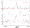 |
Fig. B.2. Same as Fig. 2 but for the observed transitions of HCOCN towards TMC-1. The red line shows the computed synthetic spectrum for propynethial assuming Tr = 5 K and N(HCOCN) = 3.5 × 1011 cm−2. |
Laboratory observed transition frequencies for HCSCN.
The rotational spectrum of HCSCN was observed in the 12–25 GHz frequency region. The molecule HCSCN was produced in a supersonic expansion at a rotational temperature of ∼2 K. Hence, only the rotational transitions with Ka = 0 and 1 could be observed. Each rotational transition is split into several hyperfine components because of the nuclear quadrupole coupling effects produced by the presence of a nitrogen nucleus, as can be seen in Fig. B.1. The interaction at the nitrogen nucleus of the quadrupole moment with the electric field gradient created by the rest of the molecular charges causes the coupling of the nuclear spin moment to the overall rotational momentum (Gordy & Cook 1984). In total, we observed 53 hyperfine components that correspond to 11 pure rotational transitions (see Table B.1). Rotational, centrifugal, and nuclear quadrupole coupling constants were determined by fitting the transition frequencies, using the SPFIT program (Pickett 1991), to a Watson’s A-reduced Hamiltonian for asymmetric top molecules, with the following form (Watson 1977): H = HR + HQ, where HR contains rotational and centrifugal distortion parameters and HQ the quadrupole coupling interactions. The energy levels involved in each transition are labelled with the quantum numbers J, Ka, Kc, and F, where F = J + I(N) and I(N)=1. The analysis rendered the experimental constants listed in Table 1. For the HC34SCN isotopic species we observed a total of 21 hyperfine components, which were analysed in the same manner as those for HCSCN. The observed frequencies are listed in Table B.2 and parameters derived from the fit in Table 1.
Laboratory observed transition frequencies for HC34SCN.
Predicted rotational constants for all the vibrationally excited states of HCSCN.
Structural optimisation calculations were carried out using the Møller-Plesset post-Hartree-Fock method, MP2 (Møller & Plesset 1934), and the Pople basis set 6–311++G(d,p) (Frisch et al. 1984). In addition, we performed anharmonic frequency calculations to estimate the rotational constants of the vibrationally excited states of HCSCN. These can be estimated using the first-order vibration-rotation constants αi that define the vibrational dependence of rotational constants Bν = Be − ∑iαi(νi + 1/2), where Bν and Be are substitutes for all three rotational constants in a given excited state and in equilibrium, respectively, and νi is the vibrational quantum number. Using the rotational constants from the merged fit shown in Table 1 and the αi constants from our calculations, we derived the rotational constants for all the vibrationally excited states of HCSCN. The results are shown in Table B.3. All the calculations were performed using the Gaussian 16 program package (Frisch et al. 2016).
As can be seen, the estimated constants for the ν9 are very close to those reported by Bogey et al. (1989). This fact and the low energy of this excited state suggest that Bogey et al. (1989) identified this state instead of the ground state of HCSCN in their experiment. The experiment conducted by Bogey et al. (1989) was done at room temperature and with the HCSCN precursor heated up to 593 K, which can also allow the population of this low energy vibrational state.
Appendix C: Cyano formaldehyde
Cyano formaldehyde, HCOCN, was detected towards Sgr B2(N) by Remijan et al. (2008). Laboratory spectroscopy on this molecule was achieved by Bogey et al. (1995). A total dipole moment of 2.8 D was adopted from ab initio calculations (Császár 1989), and the μa and μb components derived from the ratio μa/μb = 0.63 found by Bogey et al. (1995) were used. In our data only the 404 − 303 and 505 − 404 transitions are detected. They are rather weak compared to those of HCSCN. Assuming a rotational temperature of 5 K, as derived for HCSCN, all the remaining lines are below our detection limit. Figure B.2 shows the lines and the model obtained for a column density for this species of (3.5 ± 0.5) × 1011 cm−2.
Appendix D: Propynal, HCOCCH
A rich literature of laboratory work exists for this species. It has been summarised by Jabri et al. (2020). The molecule was detected in TMC-1 by Irvine et al. (1988) and towards several cold interstellar clouds by Loison et al. (2016). In TMC-1 the lines are very strong. They are shown in Fig. D.1. A fit to all the observed lines provides a rotational temperature of 4.5 ± 0.5 K and a column density for propynal of (1.5 ± 0.3) × 1012 cm−2, in excellent agreement with the value obtained by Irvine et al. (1988). It is, however, a factor of two larger than that obtained by Loison et al. (2016). This difference is probably due to the value they adopted for the rotational temperature of the observed lines, Tr = 10 K, and the fact that the energies of the upper levels of these transitions are larger than 10 K. Using their integrated line intensities and a rotational temperature of 5 K, their column density would be practically identical to ours. We would like to note that in our fit shown in Fig. D.1 the synthetic spectrum for the Ka = 0 lines has been computed for a Tr of 5 K. However, for the Ka = 1 lines it has been calculated with a rotational temperature of 4 K. This difference is within the uncertainty of the derived rotational temperature.
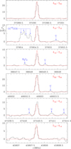 |
Fig. D.1. Same as Fig. 2 but for the observed transitions of HCOCCH towards TMC-1. The red line shows the computed synthetic spectrum for propynal assuming Tr = 5 K for the Ka = 0 lines and Tr = 4 K for the Ka = 1 lines. The resulting column density is N(HCOCCH) = 1.5 × 1012 cm−2. |
All Tables
Predicted rotational constants for all the vibrationally excited states of HCSCN.
All Figures
|
Fig. 1. Structure of cyano thioformaldehyde, HCSCN, and ethynyl thioformaldehyde, HCSCCH, also known as propynethial. |
| In the text | |
|
Fig. 2. Selected a-type transitions of HCSCN. The abscissa corresponds to the rest frequency of the lines assuming a local standard of rest velocity of the source of 5.83 km s−1. Frequencies and intensities for the observed lines are given in Table A.1. The ordinate is the antenna temperature, corrected for atmospheric and telescope losses, in millikelvin. The quantum numbers for each transition are indicated in the upper left corner of the corresponding panel. The red lines show the computed synthetic spectrum for this species for Tr = 5 K and a column density of 1.3 × 1012 cm−2. Blanked channels correspond to negative features produced in the folding of the frequency switching data. |
| In the text | |
|
Fig. 3. Same as Fig. 2 but for the b-type transitions of HCSCN. The red lines show the computed synthetic spectrum for this species for Tr = 5 K and a column density of 1.3 × 1012 cm−2. |
| In the text | |
|
Fig. 4. Same as Fig. 2 but for the observed transitions of HCSCCH towards TMC-1. The red line shows the computed synthetic spectrum for propynethial assuming Tr = 5 K and N(HCCCHS) = 3.2 × 1011 cm−2. |
| In the text | |
|
Fig. 5. Calculated fractional abundances as a function of time. Observed abundances in TMC-1 are indicated by dashed horizontal lines. |
| In the text | |
|
Fig. B.1. Fourier transform microwave spectra of HCSCN and HC34SCN showing the 30, 3–20, 2 rotational transition. The spectra show the hyperfine components, labelled with the corresponding values of quantum numbers F′–F′′, clearly resolved. The coaxial arrangement of the adiabatic expansion and the resonator axis produces an instrumental Doppler doubling. The resonance frequencies are calculated as the average of the two Doppler components. |
| In the text | |
|
Fig. B.2. Same as Fig. 2 but for the observed transitions of HCOCN towards TMC-1. The red line shows the computed synthetic spectrum for propynethial assuming Tr = 5 K and N(HCOCN) = 3.5 × 1011 cm−2. |
| In the text | |
|
Fig. D.1. Same as Fig. 2 but for the observed transitions of HCOCCH towards TMC-1. The red line shows the computed synthetic spectrum for propynal assuming Tr = 5 K for the Ka = 0 lines and Tr = 4 K for the Ka = 1 lines. The resulting column density is N(HCOCCH) = 1.5 × 1012 cm−2. |
| In the text | |
Current usage metrics show cumulative count of Article Views (full-text article views including HTML views, PDF and ePub downloads, according to the available data) and Abstracts Views on Vision4Press platform.
Data correspond to usage on the plateform after 2015. The current usage metrics is available 48-96 hours after online publication and is updated daily on week days.
Initial download of the metrics may take a while.